Electric DQ0 Library Model for Smart Grid Simulation

Abstract

This paper addresses the pressing need for advanced simulation tools in electric phasor modeling and Smart Grid-Power to X systems. The motivation for this study stems from the critical importance of enhancing the balance between performance and the detailed dynamic representation of the system behavior in the simulations. The identified problem lies in the absence of a comprehensive framework that seamlessly integrates electric phasor DQ0 components into a multi-purpose object-oriented environment. The primary objective of this research is to develop and introduce two simulation libraries, centered around the core component, Electric_DQ0. These libraries aim to establish a robust phasor-based framework, incorporating essential electric components such as sources, loads, branches, power converters, and electric machines. The main goal is to enable dynamic frequency and voltage simulations, particularly focusing on transients in alternators and facilitating Voltage and Frequency Rate of Change analysis during power production-demand imbalances. The libraries were developed within a versatile object-oriented environment, employing the Electric_DQ0 components as the foundation. Through ports, these components transmit turning frequencies, supporting the simulation of dynamic frequency and voltage. The libraries are designed to comprehensively support monophasic and triphasic systems, encompassing delta and wye connections, with a flexible neutral configuration under both balanced and unbalanced conditions. A validation case is presented to demonstrate the tool’s ability to accurately reproduce predictions when compared to one of the most widely used electrical modeling tools in the market. A study case is also presented to evaluate the toolkit’s capabilities. The study sets a specific power demand to fulfill, utilizing diverse energy sources. The obtained results showcase the libraries’ effectiveness in addressing the identified problem, providing valuable insights into their performance and applicability in real-world scenarios. The results demonstrate the efficacy of the proposed framework, delivering accurate outcomes within a reduced execution time.

1. Introduction

The swift and widespread growth of renewable energies, coupled with their integration into the grid, presents difficult challenges that demand immediate attention and resolution. Over the past decades, the penetration of renewables has escalated rapidly, characterized by a distributed expansion involving numerous power plants ranging from tens to a few hundred megawatts [1]. This surge requires a corresponding enhancement of grid integration requirements for new power plants. Anticipating the evolving needs of the renewables industry, forthcoming distributed power plants are expected to undertake grid-forming roles, employ droop techniques instead of current control, and embrace synchronized operation resembling virtual gigawatt power plants [2].

In this context, the non-manageable nature of primary resources such as sun or wind, forces renewable industries to develop storage and hybrid systems: batteries, pumped storage hydroelectric power plants [3] and, more recently, green hydrogen generation, storage and distribution [4]. Finally, the unidirectional paradigm of power grid operation, in which energy flows from producers to consumers through independent national or regional grids, is expected to change to a set of interconnected bidirectional systems suitable to combine AC and DC (Alternating and Direct Current) sections, resulting in a much more complex and control-dependent grid. Simulation tools are becoming critical in this process, especially towards Real Time (RT) applications in Hardware and Software In the Loop (HIL and SIL) solutions. These test benches minimize risks and costs compared to real equipment. Towards maximizing its performance, much effort is spent on upgrading the computing capabilities of hardware equipment and numerical solving algorithms. However, using the right mathematical approach in the modeling stage is by far the most critical step in the process. Accuracy-simplicity trade-off maximization is the key to any simulation system’s real value. By accuracy in this case we are not referring to the simulation error, but to transient phenomena that are overlooked when using the phasor approach.

The study of electric systems modeling and simulation has been approached before in detail: Good reviews of the most commonly used software environments are presented in [1,5,6]. Some works addressing the modeling of different elements that are part of the renewable generation network can also be found in the literature. In [7], electrolyzer transient models are developed in Python and simulated together with wind and solar energy sources. In [8,9] hydrogen integration with renewable energies is also modeled under different perspectives. In [10] the modeling of H₂ generation from renewable sources is also addressed, but these are simple monolithic models, control-oriented and developed ad-hoc for a specific plant.

However, the electric domain is so wide and includes so many different sub-problems that there is no single tool able to cope with it. Looking at the market, Siemens offers its co-simulation module for connecting its own PSS^®E v. 34 (Power Systems Simulator for Engineering) with PSCAD (Power Systems Computer Aided Design) from HMI (Human Machine Interface) [11]. PSS^®E and PSCAD are powerful, well-established tools that are optimized for related, yet different, simulation domains. PSS^®E has a load flow approach, suitable for large systems, whereas PSCAD is an Electro Magnetic Transient (EMT) software, used for detailed simulations of smaller systems. Other environments offer different simulation modes, with native limitations derived from that approach: MATLAB^® Simulink^® v. 2023b provides its well-known and intensively used SimPowerSystems™ v. 2023b, including its renewables section [12]. Being the most mature and advanced library for electric simulation in Simulink^®, it is the one including the PowerGui. This component allows the simulation mode, among other things, to be configured. One of these modes is Phasor, whose concept is really close to the approach set out in the library described in this paper. However, Simulink^® Phasor Mode is not suitable for some purposes, nor is it flexible. PowerGui itself is only compatible with SimPowerSystems™ components, which means that phasor mode is only usable with that library. And what is more, the list of components from SimPowerSystems™ which are compatible with phasor mode is neither long nor clear: Non linear components are not compatible (as power converters). More surprisingly, some others, such as permanent magnet synchronous machines are not compatible either as far as the authors could find. It is true that advanced users can reproduce desired topologies with phasor-compatible components, such as sources and linear components, but this alternative does not look intuitive and easy to use for average users. Additionally, the whole system must be suitable to be simulated in the selected mode and the user cannot combine different domains in the same model, in a kind of co-simulation setup. Finally, frequency in the model is fixed, constant and unique. In the latest releases, SimPowerSystems™ is included in the SimScape™ v. 2023b toolkit, as part of a wider Electrical library. The SimScape™ toolkit and its new Electrical section has a multi-domain aim but focuses on mechatronics more than the Smart Grid and energy handling. SimScape™ Electrical allows some local solver configurations for the electric section, including “Time and Frequency mode”. However, this mode is not equivalent to phasor. Alternatively, the solver step is set according to the nominal AC frequency and provides some plotting features in the phasor domain. However, the model solution is calculated through EMT equations. The SPICE-based software family is not considered in this analysis since its main focus is electronics and not so much power systems. Although its AC mode shares some common concepts with phasor analysis, differences prevail over similarities.

Another tool that employs a similar phasors approach to the library described in our paper is DPSim v 1.1.1 [13]. DPSim supports both the dynamic phasor and EMT approaches but is specifically designed for the dynamic phasor method. DPSim employs a C++ solver and a Python interface to define the model topology. It ensures fixed-time integration steps to guarantee real-time simulation for Hardware-in-the-Loop (HIL) purposes. Additionally, it is oriented towards distributed simulation and co-simulation.

In addition to the aforementioned tools, there are a number of tools specialized in the modeling and simulation of electric systems, such as DIgSILENT PowerFactory 2023 SP2, RTDS FX 2.0, ETAP 2023 (v. 22.5), etc. While these tools excel in simulating electric systems, they are oriented towards the use of built-in blocks and offer limited flexibility for modifying the causality of the model, including other domain components, or managing complex experiments. As a summary,

Table 1. Comparison of the features of different Power Systems/Smart Grid modeling tools.

Tool	Object Oriented	Closed Solution	Multidisciplary	Domain Compatibility	User Defined Models	Commercial	Phasor Based
EcosimPro Smart Grid v. 2.0 and Electric Libraries v. 1.3 [14,15]	Yes	No	Yes	Yes	Yes	Yes	Yes
Matlab Simulink SimPowerSys v. 2023b [16]	N/A	No	Yes	Yes	No	Yes	Yes
iPSL Modelica v. 2.0.0 [17]	Yes	No	Yes	Yes	Yes	No	Yes
DIgSILENT PowerFactor 2023 SP2 [18]	N/A	Yes	No	No	Yes 1	Yes	No 2
RTDS FX 2.0 [19]	N/A	Yes	No	No	Yes 3	Yes	No
ETAP-eMTCoSim 2023 (v. 22.5) [20]	N/A	Yes	No	No	Yes 4	Yes	Yes 5

¹ DIgSILENT Simulation Language (DSL) and Modelica Models. ² Possible Conversion to phasor quantities after EMT simulations. ³ RSCAD’s CBuilder. ⁴ Matlab-SimulinK (licence required). ⁵ Can be combined with EMT using co-simulation with eMTCoSim.

compares various features of the tools described so far.

In Table 1, the first column, ‘Object-Oriented Modeling’, refers to the paradigm of modeling in which models are encapsulated in components and support certain characteristics such as encapsulation, inheritance, capacity for topological connection, etc. This characteristic only applies to iPSL Modelica and EcosimPro, hence, ‘N/A’ (not applicable) is displayed for the other tools. The second column, ‘Closed Solution’, refers to tools that are open and flexible to include functions, objects, and complex structured programming. The column ‘Multidisciplinary Tool’ indicates whether the tool includes libraries for domains other than the electric one. The column ‘Domain Compatibility’ refers to the possibility of including other libraries with full compatibility and the option to connect them topologically under the same tool (excluding co-simulation). The ‘User-Defined Models’ column refers to the possibility of defining models apart from the built-in models included in the tool. While most tools offer this capability, it may not always be seamless, and some may require external software. The ‘Commercial’ column refers to software that is sold by a company for profit or is available for free. The ‘Phasor-Based’ column refers to the possibility of using the dynamic phasor mode in simulation, in addition to the EMT simulation.

An eventual software tool, able to offer a combined solution for so many different problems, disciplines and requirements in a flexible and integrated environment would be appreciated and accepted in the market and the scientific community. Additionally, the distributed and hybrid nature of the future grid, strongly suggests that purely electric modeling and simulation software will not be enough. Fluids, mechanics, thermal, and chemistry, to name but a few, must also be supported. In recent years, object-oriented general-purpose multi-domain modeling and simulation software tools have gained the upper hand and look very promising as integrated environments for solving the presented challenge in the energy area. Previous attempts to develop a power systems tool using the features of one of these well-known and validated tools were approached in Modelica-based environments. From the ObjectStab to the Spot libraries and then through the PowerSystems [21] to the last iPSL, the electric support in Modelica is well established [22] but it is still rigid and not so intuitive for beginners or even average users.

2. ELECTRIC_DQ0 and SMART_GRID Libraries

Notwithstanding the described background, as far as the authors know, this paper presents the first attempt at creating an integrated power systems simulation environment able to solve the electric problem from EMT to load flow level using the schematic drag and drop approach. The toolkit includes two different libraries: ELECTRIC_DQ0 and SMART_GRID & POWER2X, both developed in EcosimPro^®.

This software environment will provide the object-oriented multi-purpose modeling and simulation framework, with its mathematical engine and algorithms, user menus and assistants. Its paradigm perfectly fits into static or time-dependent (0D–1D) problems suitable to be described by differential algebraic equations and discrete events. Such is the case of electric analysis, where equivalent circuits are always used for abstracting expected physical behaviors. For mathematical coding, the native EcosimPro v. 6.4.24^® Language (EL) is used. Each library component encapsulates its own mathematical model and shares information with other components through smart ports, which already encapsulate flow and balance behavior for currents and voltages, respectively. Causality is also handled by the algorithms when a partition is generated. The concept of partition refers to the global analysis of all the variables and equations of the whole system, detecting inconsistencies and redundancies. Boundary conditions must be selected if the Maximum Transversal Algorithm (MTA) [23] detects more variables than equations. Then, the necessary symbolic and numeric transformations are performed in the original model looking for the explicit causality by means of the Block Lower Triangularization (BLT) Algorithm [24]. Linear loops are solved using the Lower-Upper (LU) methodology and nonlinear loops are solved using iterative methods based on Newton–Raphson. High-index problems are detected and corrected as well. The simulation settings are defined in an experiment, including duration, solver configuration, or boundary behavior, among others. The whole model is then compiled into cpp equivalent code which, in the last step, is built as a Dynamic Link Library (DLL). A graphical interface or monitor is able to load that dll, execute it and plot any variable in different ways.

In EMT-based simulation tools, every component is somehow defined by differential-algebraic equations describing resistive, inductive (or current source), or capacitive (or voltage source) behavior. In most cases this results in ordinary differential equation systems (ODE), where dependent and independent variables will be either voltages or currents. These variables are defined as time functions, being sinusoids in AC. Frequency is an input parameter stating the phase angle rate of change. These libraries or tools use discrete event handling capabilities for modeling non-linear and switching components such as diodes, transistors, or Insulated-Gate bipolar Transistors.

It is easy to foresee the numerical bottleneck that EMT modeling implies. It is not only discrete events from nonlinear components. Even when abstracting power converters to pure average sinusoidal equivalents, performance is still low and not affordable for combined simulations with higher-level systems. Variable step numerical solvers were a huge step forward in electric systems modeling and simulation but the sinusoidal nature of AC signals prevents any kind of integration step increase in the long term, losing most of the advantages of these solvers in terms of performance. Additionally, the continuous oscillating waveform of AC voltages and currents prevents any steady convergence, and therefore, any feasible solution in those applications where that is needed or at least desired: frequency domain simulation, load flow studies, optimization and parameter estimation, or even multi-domain simulation with mechanics, thermodynamics, fluids or similar. In transient simulations, these models can be solved using multi-rate techniques. This approach uses different sample rates for the different sections of the systems, depending on the time constants involved. The main advantage of multi-rate appears when using variable step methods. In those cases, the multi-rate setup prevents integration step reduction for those sections that do not need it, reducing only where it is needed. Only the necessary equations are solved at a faster rate (fundamental sample time), while slow variables can be assumed as known and constant during some samples [25].

Electric AC simulation might be approached using RMS modeling or DC equivalent, but that is not enough when the reactive component has to be considered. Alternatively, phasor modeling is the most commonly accepted solution in theoretical analysis, also widely known as Direct Quadrature equivalent. Each AC magnitude (voltage and current) is described by a turning phasor with a certain amplitude and phase. The whole analyzed system is usually moved to a turning reference frame so that the system can be described through purely algebraic steady equations. To do so, the phasor direct and quadrature components, together with the turning frequency, must be considered. Complex numbers are used for that analysis.

$$y_d\left(t\right)+j{y}_q\left(t\right)=f_{dq}\left(x_d\left(t\right),x_q\left(t\right)+j\left({x_d\left(t\right),x}_q\left(t\right)\right)\right)$$

(1)

The previously introduced generic differential algebraic equation is written again in the complex domain:

$$\frac{{dy}_d\left(t\right)}{dt}+j\frac{{dy}_q\left(t\right)}{dt}=f_{dq}\left({y_d\left(t\right),x}_d\left(t\right),{y_q\left(t\right),x}_q\left(t\right)+j\left({y_d\left(t\right),x_d\left(t\right),y}_q\left(t\right),x_q\left(t\right)\right)\right)$$

(2)

$$\frac{{dy}_d\left(t\right)}{dt}=f_d\left({y_d\left(t\right),x}_d\left(t\right),{y_q\left(t\right),x}_q\left(t\right)\right)$$

(3)

$$\frac{{dy}_q\left(t\right)}{dt}=f_q\left(\left({y_d\left(t\right),x_d\left(t\right),y}_q\left(t\right),x_q\left(t\right)\right)\right)$$

(4)

If differential terms are omitted or even neglected, the system results in a purely steady approach suitable to be described through the algebraic equation system:

$$g_d\left(x_d\left(t\right),x_q\left(t\right)\right)=h_d\left({y_d\left(t\right),y}_q\left(t\right)\right)$$

(5)

$$g_q\left(x_d\left(t\right),x_q\left(t\right)\right)=h_q\left({y_d\left(t\right),y}_q\left(t\right)\right)$$

(6)

If the reference frame is assumed to be turning at AC signal frequency, derivatives converge to zero and the solver can foresee ahead and increase the step, accelerating integration. If dynamic behavior is considered, the system results in an explicit ODE (Ordinary Differential Equation) system. If differential terms are omitted or neglected, the system turns even into a purely steady approach suitable to be described through the algebraic equation system. In electric systems, it is most often defined through linear relationships. As in the translation to electric variables example, the components storing energy according to inductive nature, will be based on the usual Faraday and Lenz laws, resulting in the following equations:

$$V\left(t\right)=L\frac{di\left(t\right)}{dt}$$

(7)

$$V\left(j\omega \right)=i\left(j\omega \right)·XL\left(j\omega \right)=\left(i_d+j{i}_q\right)·\left(X{L}_d+jX{L}_q\right)$$

(8)

$$V_d+j{V}_q=\left(i_d+j{i}_q\right)·jX{L}_q=i_d·jX{L}_q+j{i}_q·jX{L}_q=i_d·jXL-iX{L}_q$$

(9)

$$V_d=L\frac{d{i}_d\left(t\right)}{dt}-i_q·XL$$

(10)

$$V_q=L\frac{d{i}_q\left(t\right)}{dt}-i_d·XL$$

(11)

$$XL=\omega L$$

(12)

The described DQ solution is valid for monophasic or, alternatively, for balanced triphasic systems described as equivalent monophasic. To deal with monophasic systems, a fictitious component is available, but will only be used when a conversion to EMT is needed. The reason for that is the advantage of using phasors is lost when a part of the model is simulated using EMT. However, if an additional DC component is added, both wye and delta triphasic systems can be properly modeled for any neutral configuration, supporting even unbalanced conditions. This common mode, or “zero” component, will extend the system to the so-called DQ0. Properly combined, resistive, inductive, capacitive, and voltage or current sources, allow further analysis which is collected in the ELECTRIC_DQ0 library. It provides the phasor-based framework and main electric components, such as sources, loads, branches, and electric machines. Each rotative machine is described using the same approach transferred to the most convenient reference frame: Stationary, stator electric field, or rotor. Most EMT tools use Park transformation for electric machine modeling, which is based on this technique. However, unless multi-rate techniques are used, there is no big computational or performance advantage in this approach, since the EMT section will still be loading the solver.

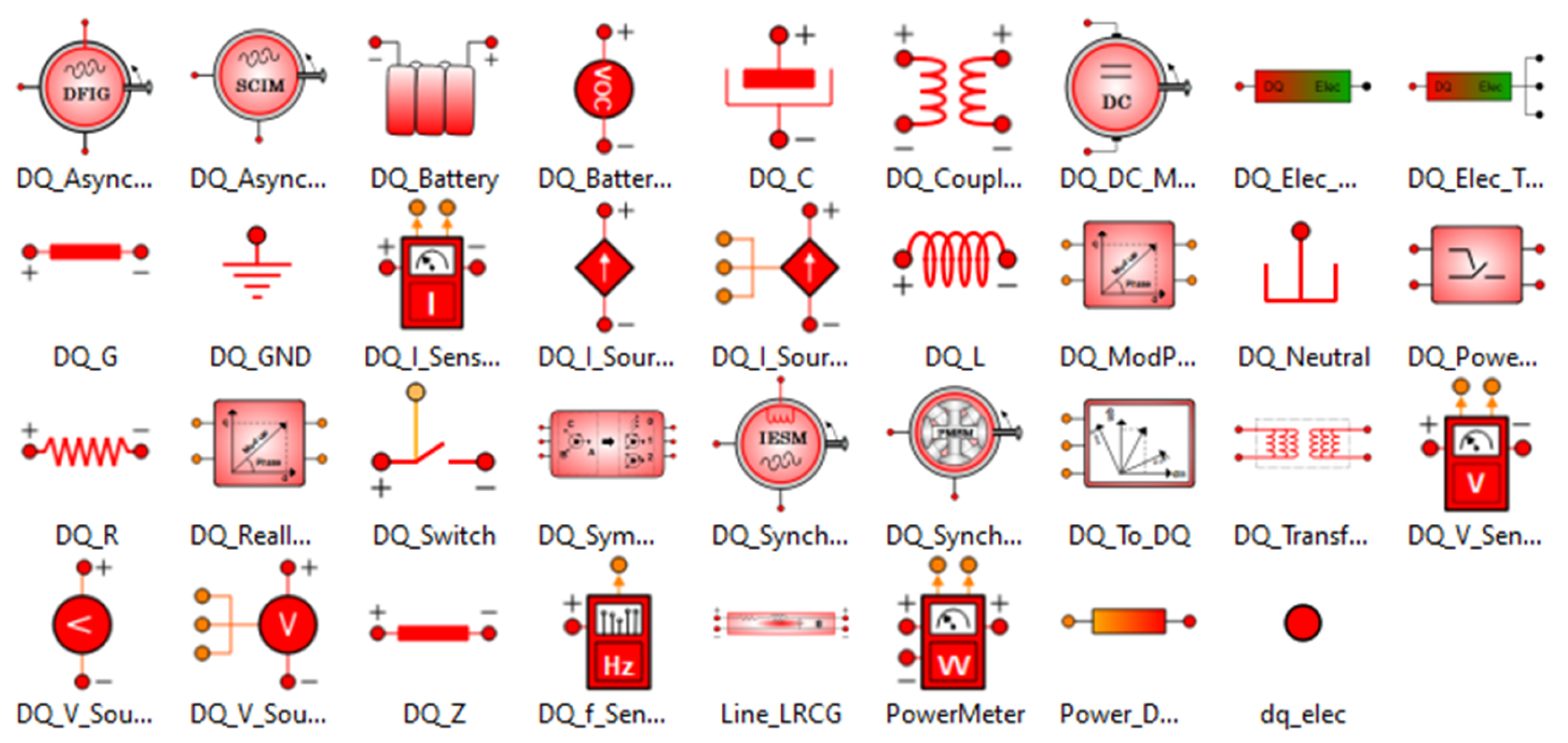
One of the relevant achievements of the ELECTRIC DQ0 library is the use of ports for sharing not only voltage and current phasor components, but also turning frequency (implicitly reference frame) and number of phases. As a result, there is no need for any global system component defining the reference framework or any other simulation conditions, unlike in Simulink^® Phasor Mode or Modelica-based solutions. This key feature allows the libraries to be used as normal EMT toolkits. It also unlocks dynamic frequency simulation, supporting dynamic transients in alternators and Frequency Rate of Change (ROCOF) analysis during production-demand power imbalances. Another derived advantage is that it is also possible to simulate sections turning at different frequencies in the same model, all converging to a steady state. This is either because the different frequencies are not directly connected, or because they are connected through AC/AC converters (frequency converters), as is increasingly the case in smart or microgrid systems. Indeed, each signal is defined as an array, each element being associated with a different frequency. In this way, the whole frequency spectrum is simulated in parallel in a single execution. If the reference frame turning frequency is null (stationary), the suggested models result in a traditional EMT modeling tool based on sinusoidal waves and ODEs. On the contrary, if dynamics are omitted, the system turns into a purely algebraic model. If it is linear, it is solvable in a single step. All the library components are suitable to be individually configured for steady or transient simulation, both in electrical and mechanical dynamics. Steady mode allows power flow applications using optimization algorithms and minimizes simulation times. A palette showing the Electric_DQ0 components and their symbols is shown in Figure 1.

3. SMART_GRID & POWER2X

As discussed in the introduction, it is accepted that the future electric grid will rely very much on non-manageable distributed production, renewable resources, storage and smart demand. To be able to model a complete smart grid, besides the electric components, the toolkit requires an extra library that includes the elements that are usually found in those distributed systems. In this regard, a set of extra components have been identified and modeled, creating a new library in the next step of the project (see Figure 2).

Most of the application cases are intended for long-time transient simulations and even steady analysis. Consequently, every component should match the expected requirements in both aspects, offering the right balance between a detailed dynamic representation of the system behavior and performance. Most of them, with more or less complexity inside, will be the primary resource to electric phasor converters for renewable energies and vice-versa, electric phasor as the resource for Power2X and storage systems. Most of these components will be configured by means of operation curves, similar to those manufacturers provide in technical documentation and data sheets. As an example of the elements that can be found in the library, some of them are introduced here.

• Photovoltaic solar panels: The PV (Photo Voltaic) cell EMT equivalent circuit is well known and widely used, including current source, PN junction and shunt and loss resistances. This unit model is usually scaled according to the number of cells, modules, panels and arrays to be considered. However, this approach is not the right choice when simulation performance becomes a priority for long-term analysis and production predictions, for example. In those cases, a PV panel detailed response is not needed, but high model performance and steady convergence is indeed the main requirement. The SMART GRID library PV panel model is based on the performance curves defining the output power vs. solar irradiance vs. DC Voltage relationship. The expected inputs are, therefore, solar irradiance and DC voltage in phasor mode. The output is a DC current in phasor mode. PV performance is defined by 3D tables expressed per unit (Figure 3). Note, that these curves can be deduced from real equipment data sheets or, alternatively, they could be generated through parametric studies performed on a traditional PV EMT model.

$$\begin{array}{cc}\hfill & Operation\_Point=Interp\left(Performance\_VS\_SunIrrad\_VS\_UDC)\right)\hfill \end{array}$$

(13)

$$\begin{array}{cc}\hfill & P_{PV}=P_s·OperationPoint\hfill \end{array}$$

(14)

$$\begin{array}{cc}\hfill & IDCOu{t}_{PV}=\frac{P_{PV}}{U_{DC}}\hfill \end{array}$$

(15)

Figure 3. Panels performance in 3D vs. Sun Irradiation vs. UDC.

Figure 3. Panels performance in 3D vs. Sun Irradiation vs. UDC.

• Wind Turbine Generator (WTG): Most of the general concepts introduced for the solar section are still valid for WTG, resulting in a similar model approach. The SMART GRID WTG model is based on performance curves defining electric power versus wind speed (Figure 4). The inputs are wind (speed and direction), AC voltage in phasor mode, and active and reactive power references. The output is AC current in phasor mode. All of them turn at grid frequency. Some operational limits are defined by parameters: maximum power vs. wind speed, input voltage operation range, time response, active-reactive power capability chart, and maximum power and current for each turbine. Operation regions are also defined, stating Cut-In, Rated, and Cut-Out wind speed.

Figure 4. Wind Turbine Generator performance vs. wind speed.

Figure 4. Wind Turbine Generator performance vs. wind speed.

$$\begin{array}{cc}\hfill & P_{WT}=Interp\left(Performance\_VS\_WindSpeed\right)\hfill \end{array}$$

(16)

$$\begin{array}{cc}\hfill & P_{WTG}=min\left(P_{WT},P_{ref}\right)\hfill \end{array}$$

(17)

$$\begin{array}{cc}\hfill & IAC\_ou{t}_{WTG}=\frac{P_{WTG}}{U_{AC}}\hfill \end{array}$$

(18)

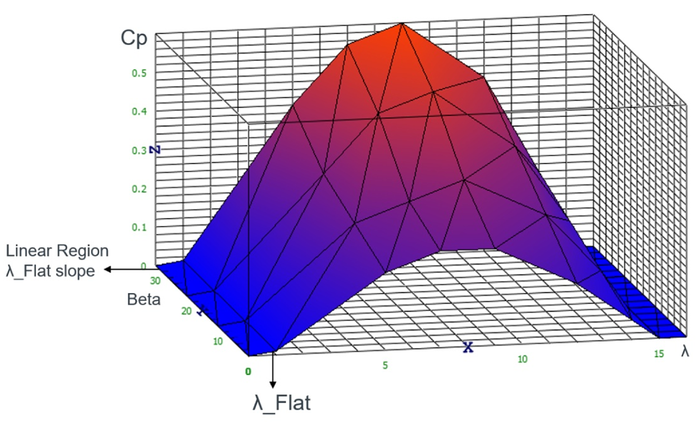
• Wind Rotor: This component describes the wind energy extraction capabilities and dynamic mechanics of a wind turbine rotor (blades, hub, gear-box and main shaft). It is based on performance curves (Cp coefficient versus $\lambda$ and $\beta$) that define mechanical power or torque versus wind speed and blade angle [26] (Figure 5). $\lambda$ describes the relationship between the wind speed and the turbine turning speed. $\beta$ is the blade angle against the wind. It is suitable for detailed wind turbine topological modeling, connecting the wind rotor to the MECHANICAL components as the prime mover for ELECTRIC_DQ0 electric machines. The main input is the wind speed and, depending on the mode, mechanic power or torque will be the output.

$$\begin{array}{cc}\hfill & P_W=0.5·\rho ·\pi ·w_s\hfill \end{array}$$

(19)

$$\begin{array}{cc}\hfill & P_{WT}=P_W·C_p\hfill \end{array}$$

(20)

Figure 5. Wind Turbine power coefficient Cp 3D curve vs. $\lambda$ vs. $\beta$.

Figure 5. Wind Turbine power coefficient Cp 3D curve vs. $\lambda$ vs. $\beta$.

• Hydroelectric: Reversible hydraulic turbine. It is based on performance and capability curves describing either turbine performance versus operation point or pump-head versus operation point. It is compatible with HIDRAULIC and MECHANICAL, and therefore, with ELECTRIC_DQ0 electric machines. In turbine mode, the expected input is the water flow, while the output is the mechanical torque. In pump mode, the expected input is the mechanical torque and the output is the pump head, and therefore, the water flow [27].
• Storage: DC batteries are based on DC Open Circuit Voltage (VOC) versus State Of Charge (SOC) curves and the equivalent circuit in phasor mode. This approach allows any cell technology to be described by different parametrizations. The output is a DC voltage (or current) in phasor mode. The expected input is a DC current (or voltage) in phasor mode.
• ${\mathit{H}}_{\mathbf{2}}$ electrolyzer and fuel cell: This component behaves as a current-sink-hydrogen-source in electrolyzer mode and as a current-source-hydrogen-sink in fuel cell mode. The hydrogen mass flow and electric current circulating through the stacks are linearly related according to the first Faraday law, which can be specifically written in dynamic form for the water direct and reverse electrolysis process.

$$\begin{array}{cc}\hfill & {\dot{m}}_{H_2}=F_{eff}·\frac{I}{2·F}M{M}_{H_2}\hfill \end{array}$$

(21)

The stack voltage depends on the operation point: the current density (J) and temperature (T). The voltage is then based on the V vs. J operation curves, as usually specified in the manufacturer’s data sheets. Following SMART_GRID library criteria, similar curves are presented to the user for the component configuration (Figure 6). The stack temperature is modeled according to the first law of thermodynamics, considering the cell stacks as an isobaric process, and therefore, using enthalpies.

This generic approach results in a flexible component, parametrizable not only as an electrolyzer or fuel cell but also more specifically, as alkaline or proton exchange membrane (PEM) variants, with either a unipolar or bipolar setup.

• Hydrogen Tank: Hydrogen is stored in a mid-pressure tank, connected to the cell stacks through specifically developed gas ports. The storage state model is also based on the first thermodynamic law, but considers the tank as an isochoric system, and therefore, uses internal energy at constant volume for the mathematical description. The stored amount, its temperature and pressure are then dynamically computed. The thermodynamic analysis falls outside the scope of this paper.
• Diesel generator: Based on the ELECTRIC_DQ0 synchronous generator in phasor mode, with mechanics based on performance curves. This is suitable for isolated operation (grid forming), or grid-connected (droop control) modes. Depending on the operation mode and point, the inputs and outputs will vary between the mechanical and electric sides, and between the voltage or current phasors.
• Electric grid: A phasor AC voltage source with dynamic frequency and amplitude evolving according to the active and reactive power balance.
• Environmental conditions: The component is used for setting environmental conditions, such as the wind speed and direction, the solar irradiance and the position of the sun, the temperature, etc. It is ready for configuration through parameters or by external weather file readings.

4. Validation of Libraries

During ELECTRIC_DQ0 and SMART_GRID toolkit development, continuous validation tests were defined and executed in an iterative debugging process. Explicit cases with known analytical solutions were defined for each component in order to confirm that the software reached the same solution. The toolkit is compatible with different execution modes, which was really useful during this process: There were specific tests comparing solutions for each method, confirming coincidence. However, during the development of a new simulation tool for any physical discipline, it is necessary to also define a robust validation plan. When possible, this validation is based on measurements and records from real systems. The same experiments are performed in real and simulated equipment and the relevant variables are compared. Ideally, they should match with some tolerance. When validation based on real references is not possible, it is also widely accepted to compare the results using a well-established simulation tool in the same area as the reference. ELECTRIC_DQ0 has been validated in two different stages. As a first step, the ELECTRIC_DQ0 phasor solution was compared with equivalent EMT models developed in EcosimPro, with positive results. In a second phase, the ELECTRIC_DQ0 was compared with one of the most popular Power Systems simulation tools, the MatlabSimulink SimScape Specialized Power Systems, which includes phasor analysis as a simulation mode. This section focuses on this second validation process.

With that aim, a validation case has been designed to include as many components as possible from different categories: Basic elements, rotative machines, transmission lines and transformers. The SimScape solution and its documentation were analyzed in detail to identify the peer components and how to properly parametrize both alternatives towards equivalence. The model suggested as the validation case resembles a scenario abstracting an off-shore wind facility, including different wind farms and turbines, transformer substation, mid distance transmission lines, on-shore grid and thermal power plant. Some are simulated as 50 MW single-equivalent inductive power plants. Some are connected to the main 25 KV 50 Hz bus. Others are connected to the same bus but at a relevant distance. Independent wind turbines are simulated as 3 MW induction generators connected individually to the main 25 KV bus. Each distance is modeled using different transmission line models: Distributed parameters RLC line, lumped parameters RLC line, and a delayed line based on the Bergeron lumped parameters model [28]. Finally, the onshore section includes a transportation line at 250 KV 50 Hz, 10 GW 250 KV 50 Hz strong grid and a thermal power plant with a 200 MVA 25 KV generator based on a synchronous alternator connected to a 250 KV grid through a 1 GW transformer.

Figure 7 and Figure 8 illustrate the model topology in both Matlab/Simulink and EcosimPro environments.

Simulink provides different streaming services. One of them automatically saves target variables in an Excel file, while EcosimPro is able to use external files and interpolate data based on local time. This methodology allows a simple graphical comparison in the EcosimPro monitor. Relevant voltages and currents in the different sections were compared with positive results.

An experiment with three different operation points is defined as a test to validate the model’s behavior: First a start-up, with a power production increase on the distant wind farms by voltage angle steps; second a power production increase in the individual wind turbines by setting slip steps on the induction generators and finally, a power production increase on the thermal power plant by a ramp on the operation angle (pulse on turning speed). The solution provided by the tools is compared in Figure 9, showing the currents in the principal bus for both models. The figure clearly shows how both models behave practically the same during transient states and for the final stationary values.

We conducted additional experiments, comparing numerous variables to validate our models. However, a detailed analysis of all the validation results is beyond the scope of this paper. Nevertheless, the consistently positive results across all cases provide confidence in the validity of the developed toolboxes.

5. Test Case

Once the toolkit and its main libraries have been introduced, a test case is presented where some of the most relevant components are used in a combined operation.

5.1. Test Case Description

The simulated scenario reproduces a grid topology, shown in Figure 10, with distributed generation based on wind, solar, reversible hydro, hydrogen, battery storage and traditional thermal generation, all connected to a grid integration component. The grid component includes a global energy demand profile through the day which must be fulfilled by the different resources.

The described system is simulated through a 24 h period, including a typical power demand profile with two load peaks at maximum activity times and lower demand during the night, no diffuse radiation has been considered. Temperature is considered constant and equal to 25 °C. The simulation starts with human activity in the early morning just before sunrise, and ends 24 h afterwards through the low activity period overnight. Solar radiation follows the usual Gauss shape, with the maximum at noon at around 900 W/m${}^2$ and a null value during the night. On the other hand, wind is assumed to be constant during the whole simulation period for this particular test case, blowing at 10 m/s in the considered area. It is expected that the control strategy manages to track the scheduled power demand accurately, presenting only short and small error gaps due to the discrete nature of the control algorithm. Regardless of the specifications, the goal of this test case is to prove the usability of the presented toolkit in similar multi-domain scenarios, where mid and long-term simulations are needed, while still keeping a good compromise between precision, reliability and realism.

The grid to which the facilities are connected operates at 25 kV AC, 50 Hz, in steady operation without Rate of Change of Voltage (ROCOV) or Rate of Change of Frequency (ROCOF). The peak power demands are 4.5 MW for active power and 500 kW for reactive power. In

Table 2. Main features of the test case facilities.

Facility	Electric Features	Other Features
Mini-Hydraulic plant	1 MW, 25 kV AC 50 Hz	Synchronous Machine Driven by ideal hydraulic machinery
PV Plant	5 MW (max) 25 kV AC 50 Hz	Centralized equivalent Inverter + Transformer
Wind Farm	4 MW 25 kV AC 50 Hz	Full Scale Converter + Transformer
Thermal: BioMass plant	100 MW 25 kV AC 50 Hz	Shynchronous machine operating at low regime 500 KW Driven by steam turbine
Battery	500 KW 200 V DC/25 kV AC 50 Hz	Inverter + Transformer Unit
H2 facility	500 KW 25 kV AC/380 V AC/200 V DC	Transformer + Rectifier Unit

, the characteristics of the main elements of the case study are shown:

5.2. PQ Control for Alternator Based Power Plants

The systems based on alternators (traditional thermal power plants and hydroelectric facilities) are controlled using operation tables. These tables are generated in the EcosimPro environment using design experiments based on optimization strategies. It is well known [29] that the active and reactive power in synchronous generators with independent field excitation can be approximated by Equations (22) and (23).

$$\begin{array}{cc}\hfill & P=\frac{3·V·E_0}{X_S}sin\left(\delta \right)\hfill \end{array}$$

(22)

$$\begin{array}{cc}\hfill & Q=\frac{3·V·E_0}{X_S}cos\left(\delta \right)-\frac{3·V^2}{X_S}\hfill \end{array}$$

(23)

There is a close relationship between active power (P) and operation angle ($\delta$) and between the stator voltage (V) and the field excitation voltage (Vf). For small angles, the dependency is even linear.

That stated, active and reactive power references are targeted in optimization experiments created on a synchronous machine item already parametrized. The field excitation voltage and operation angle are then calculated by the EcosimPro optimization algorithm. The design experiment wizard menu assists with code creation, which can be generated, accessed and customized afterward. An iterative loop is then created on top of the original case, repeating the process for a series of different power levels, with each case being associated with an index in a 2D table. Two extra 1D tables store the angle and field excitation voltage values for each sample set. This design process is intended to be executed only once for each different synchronous machine (with specific parametrization) during the toolkit development. It results in a series of values for the operation angle and field excitation voltage which are saved in xml tables. A scheme of the procedure can be seen in Figure 11.

The data generated have been post-processed and rearranged in rows and columns, for plotting only with illustrative purposes in this paper, resulting in Figure 12 and Figure 13, which confirm the stated linear dependencies.

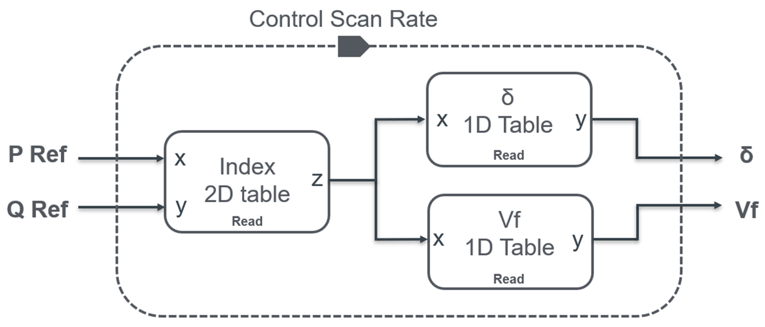
Once in operation, the synchronous machine controllers use these very same tables to perform reading operations at the control scan rate. The required active and reactive power are then used as index pointers when accessing tables, looking for the right operation angle and field excitation voltage (Figure 14). This process is executed for each synchronous machine operating in the system.

This control strategy unveils some interesting application cases, such as predictive control and maintenance when the generator does not follow the original behavior. In the test case presented in this article, the aim is purely focused on performance and predictability, and the solution exceeded expectations.

5.3. Global Control Strategy

The whole system is controlled by a global strategy, similar to the one used in real electric grids, which scans each section at different rates, depending on the control time response for that plant. Converter-based systems, such as renewables and battery storage, can track faster references. Renewables are expected to cover most of the varying power demand. On the other hand, traditional and thermal generation based on alternators will support the constant demand or baseband and will be controlled at a lower rate. The control strategy is as follows for each section:

• Traditional thermal will be the slowest resource. The power demand has a baseband, which is constant. Therefore, it is suitable to be assumed by these plants. They will deal with it at the slowest control rate, even once per day will be fast enough. Based on high-power alternators, the strategy introduced in the previous section is used.
• The PV Solar section is somehow the only exception in the control strategy because it is running in maximum power point tracking mode (MPPT), which can be understood as an open loop in this context. In essence, it means that it must generate as much as possible depending on solar irradiance. If eventually there is no power demand while there is solar energy available, it will be stored in batteries. PV power is controlled by bidirectional DCDC converters performing reference tracking. The grid connection relies on the solar DCAC inverter.
• The wind energy section must vary its operation point according to the missing power gap to be covered, once the base band and PV have been delivered to the grid under more rigid strategies. The wind power control actions are executed in a mid-speed loop.
• Hydroelectric will be able to track mid-speed references. The hydroelectric plant is also based on synchronous alternators controlled by the introduced table algorithm. In a slower loop, the hydroelectric system checks if some lack or excess of power is unbalancing the system after the baseband, solar and wind. It is crucial for the efficiency of the system that the wind control does not consider hydropower. Thus, water waste is minimized as much as possible if the wind is blowing. If there is no wind, then hydro will cover the gap in the next scan. In the meantime, faster loops will fix the small error gap.
• Finally, the fastest control loop manages the storage system, which is based on a battery bank connected to a PV DC bus through DC/DC conversion and then connected to the grid through the same PV DC/AC inverter. This loop will fix most of the residual imbalance eventually pending on the system, improving frequency and amplitude stabilities. Active power is compensated using the battery reference current at the DC side, resulting in a more stable frequency on the main AC side. Reactive compensation is shared by storage and PV power converters, while the control is performed through their AC side phi angle references. The storage system’s active and reactive control is performed in different loops, scanning at the same rate, but with some delay between them. This strategy improves reliability and ensures control of the execution order: Each new power factor is deduced with the most recent battery current set point.

The control loops run synchronously and calculate new power references for each section based on unbalanced measurements. The electric model itself is purely algebraic, and therefore, solvable without any dynamic integration, which was one of the main design requirements during the development of the ELECTRIC_DQ and SMART_GRID libraries. This approach now allows us to use the dynamic section only for control rates in a kind of interruption-based system. This solution is implemented using a fixed-step solver like EULER, which only needs two steps for each scan rate. Note, that unlike variable step solvers, EULER gives all the execution rate control to the user. At each interruption, new references are calculated for the relevant loop and the algebraic model is solved again in the very same single step. The resulting model is an extremely optimized dynamic model, equivalent to a series of steady calculations using the previous step as the initial value. A scheme of the control strategy is shown in Figure 15.

5.4. Test Case Results

The overall performance of the system can be verified by looking at the power balance of the main grid (Figure 16 and Figure 17). The power unbalance must be minimized, meaning that the different power plants are covering the demand accurately, for both active and reactive components. Note that the system is scaled down to a small area, resulting in low power levels to the order of a few MWs.

The global control strategy is intended to optimize renewable energy as much as possible. It is, therefore, expected that renewable production gets as close to the power demand as possible after the baseband; while hydro-electric limits its production in order to cover only the missing gap. This behavior can be observed in Figure 18. Renewable active power tracks the global active power demand with a constant offset equal to the baseband power, which must always be there. At maximum solar radiation times (two hours around noon), there is too much power on the system and it is wind that has to curtail production for a while with its quick response capability.

Hydraulic alternators fix small power balance gaps with their mid-speed response. The control strategy has been designed for smart usage of the different resources. It is then expected that the water consumption will be minimized with a tendency to null power production, as depicted in Figure 19. Nothing would prevent any other priority in the control strategy, such as a financial or purely electrical priority. It is also relevant to see how critical hydro-electric power is for the system, being able to produce and consume power with machinery operating as turbines or pumps. Alternatively, production based on thermal alternators keeps a constant level, resulting in the necessary base band for the grid-forming role.

The aim of the test case is to analyze the time and computational performance of the tool, evaluating their potential application in more realistic studies: 86,400 s of simulation were simulated in less than 10 s in an average personal PC, depending on the control rate tuning. These figures unveil a huge potential in different domains for energy and smart grid applications.

6. Conclusions

In the current context of the transition towards the electrification of the economy using renewable sources, there is a growing need for tools to speed up the development of new projects. To this end, the use of modeling and simulation tools is essential. This paper describes a new set of libraries for the simulation of electrical, Smart Grids and Power to X systems using the phasor approach. These libraries have been developed using an object-oriented modeling paradigm to allow non-experts in modeling and simulation to quickly build and parameterize systems. Although there are currently several alternatives available on the market for modeling these systems, as far as the authors are aware, there is no integrated multi-domain solution that allows the simulation of complete Power to X systems with a comparable accuracy-performance compromise. The article describes the existing alternatives on the market and discusses the advantages of the models developed by the authors over the existing ones. The paper shows the main features of some of the models developed. A test case has also been introduced to show the reader the capabilities of the libraries. The study case presented here shows an electrical system with a typical active and reactive power demand profile that is satisfied by different types of energy sources using a global control strategy to maximize the use of renewable energy. The results confirm how the toolkit is able to execute complex models through long periods in very short simulation times using a conventional desktop computer.