Optimization Simulation of Hydraulic Fracture Parameters for Highly Deviated Wells in Tight Oil Reservoirs, Based on the Reservoir–Fracture Productivity Coupling Model

Abstract

The production potential of highly deviated wells cannot be fully realized by conventional acid fracturing, as it can only generate a single fracture. To fully enhance the productivity of highly deviated wells, it is necessary to initiate multiple fractures along a prolonged well section to ensure the optimal number of fractures, thereby maximizing the economic returns post-stimulation. Thus, the number of fractures is a crucial parameter in the acid fracturing design of highly deviated wells. Considering factors such as the random distribution of natural fractures within the reservoir and interference between fractures during production, and, based on the oil–water two-phase flow equation, a three-dimensional reservoir–fracture production coupling model and its seepage difference model are established to simulate the production performance of highly deviated wells under varying conditions, including the number of fractures, fracture spacing, and conductivity parameters. A numerical model for the number of acid fracturing fractures in highly deviated wells is also established, in conjunction with an economic evaluation model. The simulation results indicate that the daily oil production of highly deviated wells increases with the increase in fracture number, fracture conductivity, fracture length, and reservoir permeability. However, over time, the daily oil production gradually decreases. Similarly, the cumulative production also increases with these parameters, but shows a downward trend over time. By conducting numerical simulations to evaluate the productivity and economy of highly deviated wells post-acid fracturing, it is determined that the optimal number of fractures to achieve maximum efficiency is six. The reliability of this result is confirmed by the pressure distribution cloud map of the formation after acid fracturing in highly deviated wells.

1. Introduction

To optimize the productivity of highly deviated wells post-fracturing, leverage their full potential, and enhance economic returns, it is essential to optimize the number of fractures in such wells [1,2,3,4].

As a result of the widespread adoption of horizontal well production technology in the 1980s, numerous studies have been conducted to optimize the number of hydraulic fractures in horizontal wells [5,6,7,8], resulting in its extensive application. The fundamental concept is to concentrate on analyzing the production capacity of multiple fractures (or multiple natural fractures) post-horizontal well fracturing, in tandem with evaluating the fracturing’s economic implications, with the objective of optimizing the number of fractures in horizontal wells [9,10,11,12]. Norris [13] presented a typical curve that enables the accurate prediction of horizontal well productivity, especially in single-phase porous media with multiple finite conductivity vertical fractures. Karcher et al. [14] examined the productivity of multiple fractures with infinite conductivity and introduced a calculation model to determine the production rate enhancement ratio under steady state conditions. In their study, Soliman et al. [15] established an early production model for horizontal wells with multiple finite conductivity fractures in an infinite thick reservoir. Simulation results reveal that high conductivity fractures can effectively mitigate the additional pressure drop due to the convergence of the flow lines in the vicinity of the horizontal well. According to the equation of steady state fluid flow, M.J. Economides [16] introduced a technique to estimate the productivity of oil wells by computing the pressure drop equation along the horizontal wellbore. Hegre [17] effectively clarified the correlation between the wellbore radius, fracture conductivity, fracture size, wellbore radius, fracture number, and fracture spacing, and successfully predicted the productivity of horizontal wells with lateral or vertical fractures using simulations. He introduced the notion of equivalent bore radius and conductivity correction to effectively address the problem of single-phase flow in horizontal wells. Roberts et al. [18] employed a non-Darcy flow model to simulate and assess the productivity of multiple fractures in a tight gas reservoir, concluding that the near-wellbore throttling effect would result in a significant decrease in production. When horizontal well production reaches a quasi-steady state, Guo et al. [19,20] introduced a prediction model for the productivity of multiple natural vertical fractures in a horizontal well with vertical distribution. Soliman et al. [21] examined the lateral or vertical fractures and introduced a production model for fractured horizontal wells under constant pressure conditions. Rajagopal [22] developed a mathematical model to depict the pressure dynamics of multiple fractures intersecting vertically within a horizontal well. Guo et al. [23] formulated an optimization model for the number of horizontal well fractures. They modeled the productivity of multiple fractured horizontal wells and combined it with a fractured economic assessment.

In recent years, many research efforts have been devoted to the optimization of fracture designs for highly deviated and horizontal wells. Roussel et al. [24] established a comprehensive optimization approach for hydraulic fracturing optimization of multiple fractured horizontal wells. Based on NPV (Net Present Value) maximization, they explain a methodology to help design engineers optimize several decision variables that are critical for the design of fracture treatments for unconventional reservoirs. Sun et al. [25] developed a fracture network with fractal-based techniques and demonstrated the feasibility of gridding complex natural fracture behavior with optimization-based unstructured meshing algorithms. Manriquez et al. [26] performed a novel approach to characterize reservoir and fracture pressures along the horizontal section of a well drilled in the Southwest part of the Eagle Ford unconventional shale play. Taghichian et al. [27] presented a geo-mechanical optimization procedure for toughness-dominated and viscosity-dominated regimes, based on the proposed equations that can be used for the estimation of different optimal fracturing patterns. Their optimization procedure can provide optimal simultaneous multi-stage hydraulic fracture treatment with no bias or collapse, no fracture trapping, the highest possible propagation potential in hydrocarbon-producing shale layers, and predictive proppant type/size decisions and fracture conductivity for proppant fractures. McClure et al. [28] presented a modeling study to investigate key physical processes and design considerations for a geothermal system created from multistage hydraulic stimulation, and the simulations demonstrate the impressive potential for geothermal energy production from multistage hydraulic stimulation.

These methods are primarily designed for horizontal well fracturing. The models that have been developed encompass both analytical and numerical aspects. However, the factors considered in these models are relatively degenerate. Due to their longer displacement length and capacity to traverse a wide range of reservoir horizons with diverse properties, horizontal wells are considered a special breed of highly deviated well. Therefore, optimizing the number of fractures in highly deviated well fracturing is more involved than in horizontal well fracturing and requires a more comprehensive examination of the factors involved. However, the optimization of the number of fractures in highly deviated well fracturing can also benefit from research ideas and methods used in horizontal well fracturing. Highly deviated well fracturing is a multi-fracture design that involves optimizing the number of fractures to achieve maximum economic efficiency in highly deviated well production. The distance between the fractures and the conductivity of the reservoir can affect the drainage radius between the fractures during production. Therefore, the determination of fracture spacing should not only avoid mutual interference during fracture initiation and propagation, but also minimize pressure interference during early production. Optimizing the number of fractures is a primary issue that must be accurately identified in the design of highly deviated well fracturing, in order to provide a reliable basis for the choice of fracture fluid scale and construction parameters.

In view of the unique characteristics of highly deviated wells, in this study we construct 3D equations for the oil–water two-phase flow in fractured reservoirs and their corresponding difference equations, based on an embedded discrete fracture model. Considering factors such as the random distribution of natural fractures in the reservoir and inter-fracture interference during fracture, this study numerically models the productivity of multiple fractures with different numbers, geometries, and spacing after the fracture of a highly deviated well. Combining this with an economic evaluation model for fracturing, a numerical model is established to optimize the number of fractures in highly deviated well fracturing, providing reliable data for the optimization of fracturing fluid scale and operation parameters, thus achieving the best economic results from the production increase and modification of the reservoir.

2. Three-Dimensional Reservoir–Fracture Productivity Coupling Model

The three-dimensional coupled model of oil reservoir and fracture productivity comprises the reservoir matrix flow model, fracture flow model, and the flow exchange model between fractures and the reservoir matrix. The reservoir matrix flow model and fracture flow model are, respectively, two-dimensional and one-dimensional models. In the construction of the flow exchange model between fractures and the reservoir matrix, an embedded discrete fracture model was employed [29,30]. This model, when addressing the flow exchange between fractures and the reservoir, offers significant advantages. It allows for the establishment of the relationship between fractures and the reservoir without the need for local grid refinement, thus reducing the complexity of grid division, the number of grids, and model solution time.

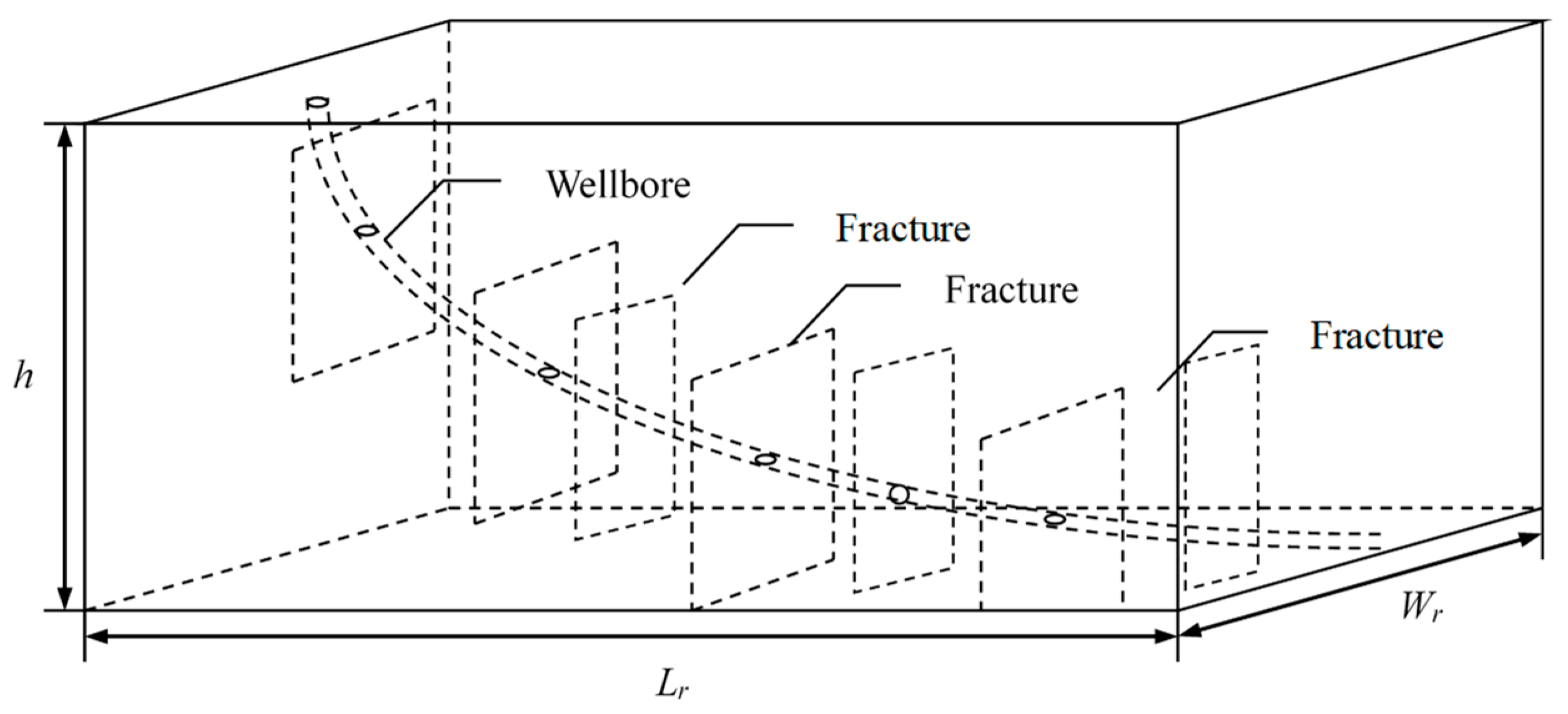
2.1. Assumptions and Physical Model

The black oil model in the reservoir numerical simulation is a fully implicit, three-dimensional, and three-phase general model. The widely used black oil model has been employed in numerical simulations of pressure-induced productivity in highly deviated wells, considering the actual condition of the reservoir in which the highly deviated well is located. A schematic diagram of the physical model of the high-inclination trap is shown in Figure 1, which is derived from the following assumptions:

(1)

The reservoir is rectangular in shape and the fluid within it is in an isothermal state of percolation.

(2)

The reservoir pressure is consistently larger than the saturation pressure, and there is no unconfined gas within the reservoir. The fluid inside the reservoir adheres to a two-phase flow of oil and water, following the Darcy flow regime.

(3)

Highly deviated wells are primarily cemented, disregarding the effect of the borehole on production, and relying solely on perforations or fractures for production.

(4)

The fracture fully penetrates the production layer and is symmetrically distributed around the center of the production layer, regardless of the transverse permeability of the reservoir. However, vertical gravity and the permeability of the production layer must be taken into account.

(5)

During the simulation evaluation, the fracture is considered as a component of the reservoir, and fracture amplification is employed to introduce the fracture directly into the reservoir for immediate simulation.

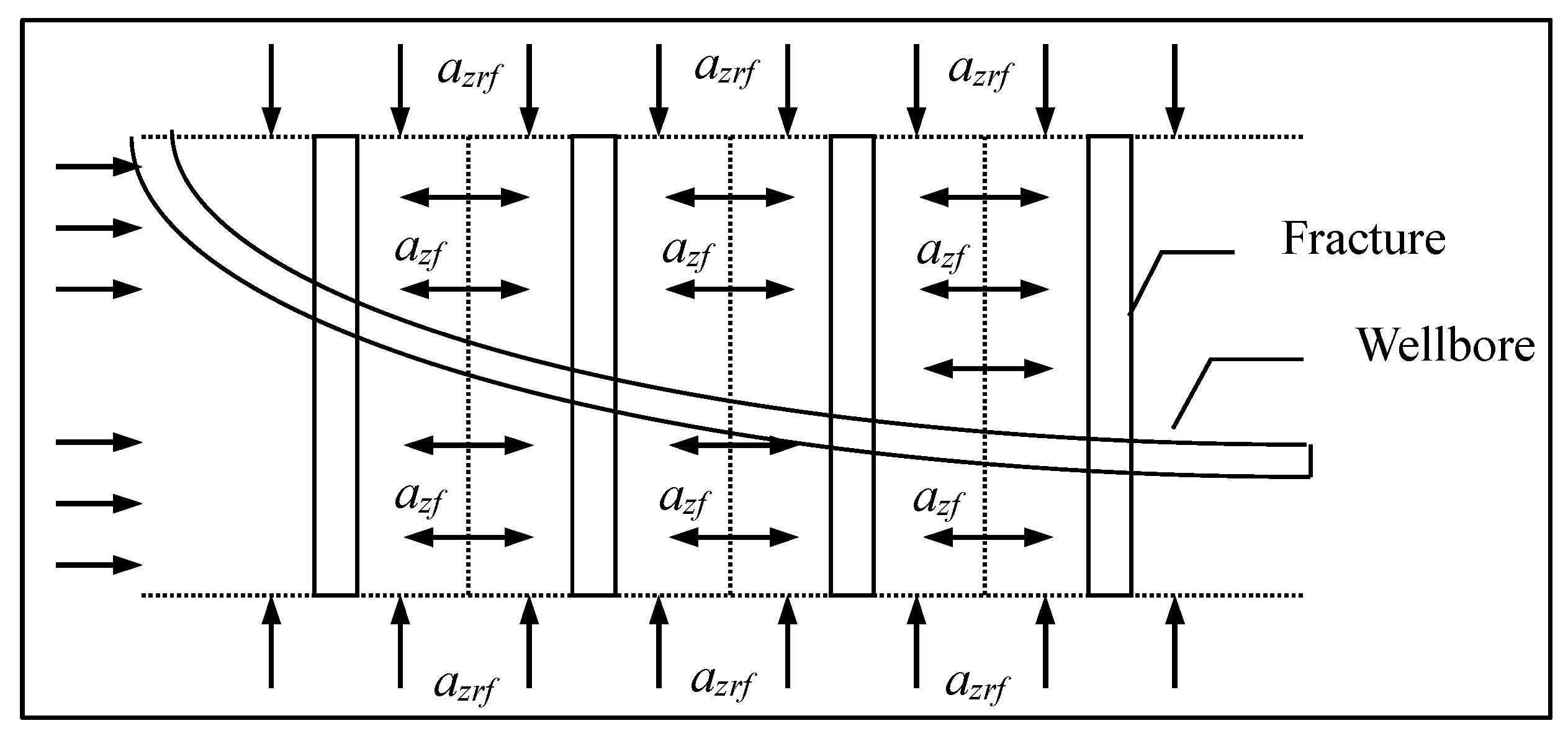
2.2. Embedded Discrete Fracture Model

The embedded discrete fracture model (EDFM) is a method to simplify the meshing of the solution region of the fracture flow process by dimensionality reduction [31]. The reservoir simulated in this paper is a two-dimensional plane model, so the fractures are treated as one-dimensional. According to the principle of EDFM, the two-dimensional reservoir can use an orthogonal structured grid to discretize the reservoir area, while the corresponding fractures, which are treated as one-dimensional, are divided into multiple line segment units by the reservoir grid interface. These line segment units are considered as “line source sink items” embedded within the continuous matrix. Currently, the reservoir and fractures each utilize distinct grid systems. The reservoir employs an orthogonal structured grid, while the fractures are represented by a line segment grid. The model construction for each is illustrated in Figure 2. In practical scenarios, fractures possess a specific width and separate the matrix along their length, rendering the matrix on either side of the fracture discontinuous. In the EDFM framework, fractures, now considered one-dimensional, no longer maintain their actual width. The embedded fractures do not actually intersect the matrix but exist as “line source sink terms,” preserving the continuity of the matrix on either side of the fracture. The true physical volume of the fracture is redefined within a distinct grid system.

Through fracture identification techniques (such as seismic, logging, and outcrop core observation), the original data of natural fracture distribution in the reservoir are obtained. By employing probability statistics methods, the statistical analysis of this data is conducted to derive the parameters of the natural fracture distribution. Subsequently, software equipped with various probability distribution functions is utilized for programming to generate the plane model of the discrete fracture network within the reservoir model, as illustrated in Figure 3.

2.3. Three-Dimensional Single-Fracture Percolation Model for Oil and Water Phases

The effects of gas are not considered for the oil and water phases based on physical models of borehole fracture systems in highly deviated wells and associated assumptions. The physical parameters of the reservoir vary from one production zone to another, due to the lengthy borehole displacement and the numerous production zones traversed. In view of these circumstances, in this paper we use a 3D model of oil–water two-phase percolation to model the production performance of a reservoir after stimulation:

$$V_o=-\frac{K{K}_{ro}}{{\mu }_o}(\nabla P_o-{\gamma }_o\nabla D)$$

(1)

$$V_w=-\frac{K{K}_{rw}}{{\mu }_w}(\nabla P_w-{\gamma }_w\nabla D)$$

(2)

where V_o and V_w are the oil phase and water phase flow velocities, respectively, m/s. K is the air permeability of a low permeability core, m². K_ro and K_rw are the relative permeability of the oil and water phases, respectively. μ_o and μ_w are the viscosity of the oil and water phases, respectively, Pa·s. P_o and P_w are the starting pressure gradient of the oil and water phases, respectively Pa/m. D is the pressure gradient of gravity, Pa/m. ${\gamma }_o$ and ${\gamma }_w$ are the relative density of the oil and water phases, respectively, Dimensionless.

Based on the principle of matter balance, the equations for the matter balance of the oil–water two-phase are given as follows:

$$-\nabla \left({\rho }_o{V}_o\right)=\frac{\partial \left(\phi {\rho }_o{S}_o\right)}{\partial t}$$

(3)

$$-\nabla \left({\rho }_w{V}_w\right)=\frac{\partial \left(\phi {\rho }_w{S}_w\right)}{\partial t}$$

(4)

where, $\phi$ is the porosity, %. So and Sw are the oil saturation and water saturation, respectively. ${\rho }_o$ and ${\rho }_w$ are the relative density of the oil and water phases, respectively, kg/m³.

By combining Equations (1) and (4), we derive the differential equation for the oil–water two-phase flow:

Percolation equation for the oil phase:

$$\nabla \left[\frac{K{K}_{ro}{\rho }_o}{{\mu }_o}\left(\nabla {\rho }_o-{\gamma }_{og}\nabla D\right)\right]=\frac{\partial \left(\phi {\rho }_o{S}_o\right)}{\partial t}$$

(5)

Seepage equation for the water phase:

$$\nabla \left[\frac{K{K}_{rw}{\rho }_w}{{\mu }_w}\left(\nabla {\rho }_w-{\gamma }_w\nabla D\right)\right]=\frac{\partial \left(\phi {\rho }_w{S}_w\right)}{\partial t}$$

(6)

After developing a 3D oil–water two-phase flow model for highly deviated wells, the key trick is to determine an efficient method to solve the reservoir flow model.

2.4. The Mathematical Model for the Phase Difference in Oil within Three-Dimensional Reservoirs

By utilizing the IMPES (IMplicit Pressure Explicit Saturation) method, the oil phase (Formula (5)) of the three-dimensional two-phase flow model undergoes spatial differentiation, resulting in the derivation of the given equation after simplification and rearrangement.

$$\begin{gathered} \frac{1}{\mathsf{\Delta }{X}_i}\left[{\left(\frac{K{K}_{ro}{\rho }_o}{{\mu }_o}\right)}_{i+\frac{1}{2}}^n\left(\frac{P_{i+1}^{n+1}-P_i^{n+1}}{\mathsf{\Delta }{X}_{i+\frac{1}{2}}}-{\gamma }_{oi+\frac{1}{2}}^n\frac{D_{i+1}-D_i}{\mathsf{\Delta }{X}_{i+\frac{1}{2}}}\right) \\ +{\left(\frac{K{K}_{ro}{\rho }_o}{{\mu }_o}\right)}_{i-\frac{1}{2}}^n\left(\frac{P_{i-1}^{n+1}-P_i^{n+1}}{\mathsf{\Delta }{X}_{i-\frac{1}{2}}}-{\gamma }_{oi-\frac{1}{2}}^n\frac{D_{i-1}-D_i}{\mathsf{\Delta }{X}_{i-\frac{1}{2}}}\right)\right] \\ +\frac{1}{\mathsf{\Delta }{Y}_j}\left[{\left(\frac{K{K}_{ro}{\rho }_o}{{\mu }_o}\right)}_{j+\frac{1}{2}}^n\left(\frac{P_{j+1}^{n+1}-P_j^{n+1}}{\mathsf{\Delta }{Y}_{j+\frac{1}{2}}}-{\gamma }_{oj+\frac{1}{2}}^n\frac{D_{j+1}-D_j}{\mathsf{\Delta }{Y}_{j+\frac{1}{2}}}\right) \\ +{\left(\frac{K{K}_{ro}{\rho }_o}{{\mu }_o}\right)}_{j-\frac{1}{2}}^n\left(\frac{P_{j-1}^{n+1}-P_j^{n+1}}{\mathsf{\Delta }{Y}_{j-\frac{1}{2}}}-{\gamma }_{oj-\frac{1}{2}}^n\frac{D_{j-1}-D_j}{\mathsf{\Delta }{Y}_{j-\frac{1}{2}}}\right)\right] \\ +\frac{1}{\mathsf{\Delta }{Z}_k}\left[{\left(\frac{K{K}_{ro}{\rho }_o}{{\mu }_o}\right)}_{k+\frac{1}{2}}^n\left(\frac{P_{k+1}^{n+1}-P_k^{n+1}}{\mathsf{\Delta }{Z}_{k+\frac{1}{2}}}-{\gamma }_{ok+\frac{1}{2}}^n\frac{D_{k+1}-D_k}{\mathsf{\Delta }{Z}_{k+\frac{1}{2}}}\right) \\ +{\left(\frac{K{K}_{ro}{\rho }_o}{{\mu }_o}\right)}_{k-\frac{1}{2}}^n\left(\frac{P_{k-1}^{n+1}-P_k^{n+1}}{\mathsf{\Delta }{Z}_{k-\frac{1}{2}}}-{\gamma }_{ok-\frac{1}{2}}^n\frac{D_{k-1}-D_k}{\mathsf{\Delta }{Z}_{k-\frac{1}{2}}}\right)\right] \\ =\frac{1}{\mathsf{\Delta }t}\left[{\left(\phi {\rho }_o{S}_o\right)}^{n+1}-{\left(\phi {\rho }_o{S}_o\right)}^n\right] \end{gathered}$$

(7)

where

$$T_{xoi+\frac{1}{2}}=\frac{\mathsf{\Delta }{Y}_j\mathsf{\Delta }{Z}_k}{\mathsf{\Delta }{X}_{i+\frac{1}{2}}}{{\left(\frac{K{K}_{ro}{\rho }_o}{{\mu }_o}\right)}^n}_{i+\frac{1}{2}}, T_{xoi-\frac{1}{2}}=\frac{\mathsf{\Delta }{Y}_j\mathsf{\Delta }{Z}_k}{\mathsf{\Delta }{X}_{i-\frac{1}{2}}}{{\left(\frac{K{K}_{ro}{\rho }_o}{{\mu }_o}\right)}^n}_{i-\frac{1}{2}}$$

$$T_{yoj+\frac{1}{2}}=\frac{\mathsf{\Delta }{X}_i\mathsf{\Delta }{Z}_k}{\mathsf{\Delta }{Y}_{j+\frac{1}{2}}}{{\left(\frac{K{K}_{ro}{\rho }_o}{{\mu }_o}\right)}^n}_{j+\frac{1}{2}}, T_{yoj-\frac{1}{2}}=\frac{\mathsf{\Delta }{X}_i\mathsf{\Delta }{Z}_k}{\mathsf{\Delta }{Y}_{j-\frac{1}{2}}}{{\left(\frac{K{K}_{ro}{\rho }_o}{{\mu }_o}\right)}^n}_{j-\frac{1}{2}}$$

$$T_{zok+\frac{1}{2}}=\frac{\mathsf{\Delta }{X}_i\mathsf{\Delta }{Y}_j}{\mathsf{\Delta }{Z}_{k+\frac{1}{2}}}{{\left(\frac{K{K}_{ro}{\rho }_o}{{\mu }_o}\right)}^n}_{k+\frac{1}{2}}, T_{zok-\frac{1}{2}}=\frac{\mathsf{\Delta }{X}_i\mathsf{\Delta }{Y}_j}{\mathsf{\Delta }{Z}_{k-\frac{1}{2}}}{{\left(\frac{K{K}_{ro}{\rho }_o}{{\mu }_o}\right)}^n}_{k-\frac{1}{2}}$$

Then, Formula (7) can be simplified to:

$$\begin{gathered} T_{xoi+\frac{1}{2}}\left[P_{i+1}^{n+1}-P_i^{n+1}-{\gamma }_{oi+\frac{1}{2}}^n\left(D_{i+1}-D_i\right)\right]+T_{xoi-\frac{1}{2}}\left[P_{i-1}^{n+1}-P_i^{n+1}-{\gamma }_{oi-\frac{1}{2}}^n\left(D_{i-1}-D_i\right)\right] \\ +T_{yoj+\frac{1}{2}}\left[P_{j+1}^{n+1}-P_j^{n+1}-{\gamma }_{oj+\frac{1}{2}}^n\left(D_{j+1}-D_j\right)\right] \\ +T_{yoj-\frac{1}{2}}\left[P_{j-1}^{n+1}-P_j^{n+1}-{\gamma }_{oj-\frac{1}{2}}^n\left(D_{j-1}-D_j\right)\right] \\ +T_{zok+\frac{1}{2}}\left[P_{k+1}^{n+1}-P_k^{n+1}-{\gamma }_{ok+\frac{1}{2}}^n\left(D_{k+1}-D_k\right)\right] \\ +T_{zok-\frac{1}{2}}\left[P_{k-1}^{n+1}-P_k^{n+1}-{\gamma }_{ok-\frac{1}{2}}^n\left(D_{k-1}-D_k\right)\right]=\frac{V_{ijk}}{\mathsf{\Delta }t}\left[{\left(\phi {\rho }_o{S}_o\right)}^{n+1}-{\left(\phi {\rho }_o{S}_o\right)}^n\right] \end{gathered}$$

(8)

where

$${\gamma }_{oi+\frac{1}{2}}^n=\frac{1}{2}\left({\gamma }_{oi+1}^n+{\gamma }_{oi}^n\right), {\gamma }_{oi-\frac{1}{2}}^n=\frac{1}{2}\left({\gamma }_{oi-1}^n+{\gamma }_{oi}^n\right)$$

$${\lambda }_{oi+\frac{1}{2}}={\left(\frac{K{K}_{ro}{\rho }_o}{{\mu }_o}\right)}_{i+\frac{1}{2}},{\lambda }_{oi-\frac{1}{2}}={\left(\frac{K{K}_{ro}{\rho }_o}{{\mu }_o}\right)}_{i-\frac{1}{2}}$$

$${\lambda }_{oj+\frac{1}{2}}={\left(\frac{K{K}_{ro}{\rho }_o}{{\mu }_o}\right)}_{j+\frac{1}{2}},{\lambda }_{oj-\frac{1}{2}}={\left(\frac{K{K}_{ro}{\rho }_o}{{\mu }_o}\right)}_{j-\frac{1}{2}}$$

$${\lambda }_{ok+\frac{1}{2}}={\left(\frac{K{K}_{ro}{\rho }_o}{{\mu }_o}\right)}_{k+\frac{1}{2}},{\lambda }_{ok-\frac{1}{2}}={\left(\frac{K{K}_{ro}{\rho }_o}{{\mu }_o}\right)}_{k-\frac{1}{2}}$$

where λ is the flow coefficient, and by analogy, ${\gamma }_{oj+\frac{1}{2}}^n,{\gamma }_{oj-\frac{1}{2}}^n,{\gamma }_{ok+\frac{1}{2}}^n,{\gamma }_{ok-\frac{1}{2}}^n$

Where, for absolute permeability, $K_{i+\frac{1}{2}}=\frac{2K_{\mathrm{i}}{K}_{\mathrm{i}+1}}{K_{\mathrm{i}}+{\mathrm{K}}_{\mathrm{i}+1}}$, ${\mathrm{K}}_{\mathrm{i}-\frac{1}{2}}=\frac{2{\mathrm{K}}_{\mathrm{i}}{\mathrm{K}}_{\mathrm{i}-1}}{{\mathrm{K}}_{\mathrm{i}}+{\mathrm{K}}_{\mathrm{i}-1}}$, and by analogy, ${\mathrm{K}}_{\mathrm{j}+\frac{1}{2}}$, ${\mathrm{K}}_{\mathrm{j}-\frac{1}{2}}$, ${\mathrm{K}}_{\mathrm{k}+\frac{1}{2}}$, ${\mathrm{K}}_{\mathrm{k}-\frac{1}{2}}$. $\phi$ is the porosity, %. S_o and S_w are the oil saturation and water saturation, respectively. ${\rho }_o$ and ${\rho }_w$ are the relative density of the oil and water phases, respectively, kg/m³. ${\gamma }_o$ and ${\gamma }_w$ are the relative density of oil and water phases, respectively, Dimensionless.

The upstream value of relative permeability K_ro is employed, with flow direction from high pressure to low pressure. The high-pressure point has been identified, and the surrounding pressure around the node must be evaluated. Since ρ_o and μ_o only have time values and not spatial values, it is sufficient to use the previous time step.

To further simplify the formula,

$$\begin{array}{c}{T}_{zok-\frac{1}{2}}\left(P_{k-1}^{n+1}-{\gamma }_{ok-\frac{1}{2}}^n{D}_{k-1}\right)+T_{yoj-\frac{1}{2}}\left(P_{j-1}^{n+1}-{\gamma }_{oj-\frac{1}{2}}^n{D}_{j-1}\right)+T_{xoi-\frac{1}{2}}\left(P_{i-1}^{n+1}-{\gamma }_{oi-\frac{1}{2}}^n{D}_{i-1}\right)\hfill \\ -\left(T_{zok-\frac{1}{2}}+T_{yoj-\frac{1}{2}}+T_{xoi-\frac{1}{2}}+T_{xoi+\frac{1}{2}}+T_{yoj+\frac{1}{2}}+T_{zok+\frac{1}{2}}\right)P_{ijk}^{n+1}\hfill \\ {+(\gamma }_{ok-\frac{1}{2}}^n \ast T_{zok-\frac{1}{2}}+{\gamma }_{oj-\frac{1}{2}}^n \ast T_{yok-\frac{1}{2}}+{\gamma }_{oi-\frac{1}{2}}^n \ast T_{xoi-\frac{1}{2}}+{\gamma }_{oi+\frac{1}{2}}^n \ast T_{xoi+\frac{1}{2}}+{\gamma }_{oy+\frac{1}{2}}^n\hfill \\ \ast T_{yoj+\frac{1}{2}}+{\gamma }_{ok+\frac{1}{2}}^n+ \ast T_{zok+\frac{1}{2}})D_{ijk}+T_{xoi+\frac{1}{2}}\left(P_{i+1}^{n+1}-{\gamma }_{oi+\frac{1}{2}}^n{D}_{i+1}\right)\hfill \\ +T_{yoj+\frac{1}{2}}\left(P_{j+1}^{n+1}-{\gamma }_{oj+\frac{1}{2}}^n{D}_{j+1}\right)+T_{zok+\frac{1}{2}}\left(P_{k+1}^{n+1}-{\gamma }_{ok+\frac{1}{2}}^n{D}_{k+1}\right)\hfill \\ =\frac{V_{ijk}\phi {\rho }_o}{\mathsf{\Delta }t}\left({S_o}^{n+1}-{S_o}^n\right)\hfill \end{array}$$

(9)

2.5. Three-Dimensional Spatial Water Difference Fractional Model

Similar to the approach used to create the 3D oil phase differential model, the aqueous phase obeys the following equations:

$$\begin{array}{c}{T}_{zok-\frac{1}{2}}{P}_{k-1}^{n+1}+T_{yoj-\frac{1}{2}}{P}_{j-1}^{n+1}+T_{xoi-\frac{1}{2}}{P}_{i-1}^{n+1}\hfill \\ -\left(T_{zok-\frac{1}{2}}+T_{yoj-\frac{1}{2}}+T_{xoi-\frac{1}{2}}+T_{xoi+\frac{1}{2}}+T_{yoj+\frac{1}{2}}+T_{zok+\frac{1}{2}}\right)P_{ijk}^{n+1}+T_{xoi+\frac{1}{2}}{P}_{i+1}^{n+1}\hfill \\ +T_{yoj+\frac{1}{2}}{P}_{j+1}^{n+1}+T_{zok+\frac{1}{2}}{P}_{k+1}^{n+1}-T_{zok-\frac{1}{2}}{\gamma }_{ok-\frac{1}{2}}^n{D}_{k-1}-T_{yoj-\frac{1}{2}}{\gamma }_{oj-\frac{1}{2}}^n{D}_{j-1}\hfill \\ -T_{xoi-\frac{1}{2}}{\gamma }_{oi-\frac{1}{2}}^n{D}_{i-1}\hfill \\ +({\gamma }_{ok-\frac{1}{2}}^n{T}_{zok-\frac{1}{2}}+{\gamma }_{oj-\frac{1}{2}}^n{T}_{yoj-\frac{1}{2}}+{\gamma }_{oi-\frac{1}{2}}^n{T}_{xoi-\frac{1}{2}}+{\gamma }_{oi+\frac{1}{2}}^n{T}_{xoi+\frac{1}{2}}+{\gamma }_{oy+\frac{1}{2}}^n{T}_{yoj+\frac{1}{2}}\hfill \\ {+\gamma }_{ok+\frac{1}{2}}^n{T}_{zok+\frac{1}{2}})D_{ijk}-T_{xoi+\frac{1}{2}}{\gamma }_{oi+\frac{1}{2}}^n{D}_{i+1}-T_{yoj+\frac{1}{2}}{\gamma }_{oj+\frac{1}{2}}^n{D}_{j+1}-T_{zok+\frac{1}{2}}{\gamma }_{ok+\frac{1}{2}}^n{D}_{k+1}\hfill \\ =\frac{V_{ijk}}{\mathsf{\Delta }t}\left[S_o{\rho }_o\phi \left(C_r+C_o\right)\left(P_o^{n+1}-P_o^n\right)+\phi {\rho }_o\left(S_o^{n+1}-S_o^n\right)\right]\hfill \end{array}$$

(10)

Utilizing ${\mathrm{P}}_{\mathrm{w}}^{\mathrm{n}+1}={\mathrm{P}}_{\mathrm{o}}^{\mathrm{n}+1}-{\mathrm{P}}_{\mathrm{c}}^{\mathrm{n}}$ and ${\mathrm{S}}_{\mathrm{w}}^{\mathrm{n}}=1-{\mathrm{S}}_{\mathrm{o}}^{\mathrm{n}}$ substitution, where ${\mathrm{P}}_{\mathrm{c}}^{\mathrm{n}}$ is capillary pressure at time n.

2.6. Differential Mathematical Model of Oil–Water Two-Phase Seepage in a Three-Dimensional Reservoir

By using the above formulation, the differential equation for the spatial oil–water two-phase percolation model in a 3D reservoir reduces to the following:

$$a_{ijk}{P}_{k-1}^{n+1}+b_{ijk}{P}_{j-1}^{n+1}+c_{ijk}{P}_{i-1}^{n+1}+d_{ijk}{P}_{ijk}^{n+1}+e_{ijk}{P}_{i+1}^{n+1}+f_{ijk}{P}_{j+1}^{n+1}+g_{ijk}{P}_{k+1}^{n+1}+h_{ijk}=0$$

(11)

where, a_ijk, b_ijk, c_ijk, d_ijk, e_ijk, f_ijk, g_ijk, and h_ijk are coefficients.

The percolation differential equations are solved by partitioning the entire reservoir into grids, resulting in a set of 7-diagonal equations, which are then solved iteratively using a linear set of equation approximations.

2.7. Initial Conditions and Boundary Conditions

Taking into account the actual reservoir situation, the initial condition for the percolation differential Equation (12) is:

$$P\left(x,y,z,0\right)=\phi \left(x,y,z\right)$$

(12)

$$S_w=S_{wo}\left(x,y,z\right)$$

(13)

There are internal and external boundary conditions for defining the limits of a system. Since the wellbore of a highly deviated well is typically cemented, it can be regarded as a sealed condition, thereby imposing an internal boundary condition of $\frac{\partial \mathrm{P}}{\partial \mathrm{n}}{|}_{\mathrm{G}}=0$. In this context, “n” denotes the normal direction, and both the vertical and horizontal sections of the wellbore are considered as closed boundaries.

There are two types of external boundary conditions: the closed boundary condition and the constant pressure boundary condition, which is determined according to the specific situation. The boundary condition of closed boundary is $\frac{\partial \mathrm{P}}{\partial \mathrm{n}}{|}_{\mathrm{G}}=0$, whereas the boundary condition of constant pressure is ${\mathrm{P}}_{\mathrm{G}}=\mathrm{C}$.

Because hydraulic bag completion and perforated fracturing are performed primarily in highly deviated wells, only fracture production is considered when evaluating post-fracking productivity, disregarding the remaining area of the wellbore as a closed boundary.

$$Q=\frac{2\pi KW}{\mu }\left(\frac{P_{ijk}-P_{wf}}{\mathit{ln}\frac{r_e}{r_w}+S}\right)$$

(14)

$$K=\sqrt{K_y{K}_z}$$

(15)

For heterogeneous reservoir grids:

$$r_e=\frac{0.28\sqrt{(K_z/K_y{)}^{0.5}\mathsf{\Delta }{y}^2+(K_y/K_z{)}^{0.5}\mathsf{\Delta }{z}^2}}{(K_z/K_y{)}^{0.5}+(K_y/K_z{)}^{0.5}}$$

(16)

For homogeneous reservoir grids:

$$r_e=0.14\sqrt{\mathsf{\Delta }{x}^2+\mathsf{\Delta }{y}^2}$$

(17)

where W is the fracture width, m; S is the formation skin factor, dimensionless; P_ijk is the fluid pressure in the grid block where the center point of the fracture is located, MPa; P_wf is the flowing pressure at the bottom of the well, MPa; r_e is the equivalent radius of radial flow outer boundary radius, m; K_x, K_y, and K_z are the reservoir permeability in the X, Y, and Z directions, respectively, mD.

The permeability can be reduced at a particular diversion capacity by enlarging the fracture into a grid with a single production term at the fracture center, resulting in a final yield that is the sum of the yields from each fracture.

During the initial phase of production following hydraulic fracturing, every fracture contributes fluid from its distinct control area, denoted as a_zf (as illustrated in Figure 2). Moreover, each area does not impede the flow of the other, thereby allowing for an infinite boundary production. As production progresses, the fracture supply area will expand beyond its individual control, leading to inter-fracture interference and altered production outcomes. In this case, the constant pressure production method is employed to determine the amount of fluid flowing into each direct control zone, a_zf, at any given time within the common control zone. As production progresses, the pressure within the direct control zone, a_zf, of each fracture decreases, and the pressure profile is determined by numerical simulations. The flow volume of fluid from the common control area a_zrf into the direct control area a_zf is computed, and the multi-fracture production capacity after fracturing can be ascertained. These processes can be implemented in numerical simulations.

The pressure distribution and production at various times can be determined by applying the method described above. The production obtained from numerical simulations is compared with that obtained using analytical solutions to validate the results. Finally, the mesh is subdivided in each direction.

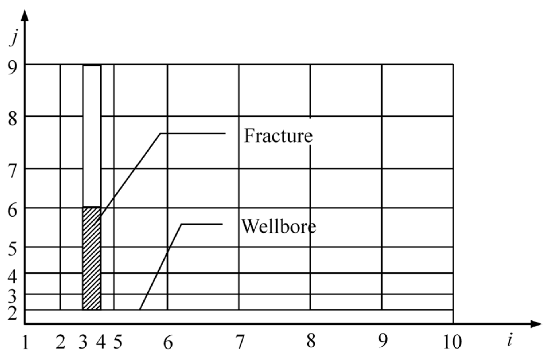
2.8. Reservoir Grid System Division

In Figure 4, a schematic diagram of the horizontal section of fractures and wellbore in a highly deviated well in a reservoir is presented. The reservoirs are classified into two distinct types of zones, each with its own independently controlled zone, a_zf, and common controlled zone, a_zrf.

Obtaining analytical solutions for 3D oil–water two-phase flow models in highly deviated wells is a challenging task. In this paper, an implicit finite difference approach is used to develop a flow difference model. Figure 5 shows a schematic diagram of a reservoir–fracture mesh for the fracture single-wing splitting of an unequal-spacing reservoir–fracture system.

The number of grids and their respective locations are determined based on the number and location of the simulated fractures. The computational load can be reduced while maintaining a certain level of accuracy by fixing the number of grids at 40 between fractures in advance. Simultaneously, the number of grids between the fractures can be input to maximize the number of grids within the allowed limits of the computer, thereby guaranteeing computational accuracy. Due to the expected pressure interference between fractures after a certain production period, the grid in the vicinity of the fracture should be identified. For this purpose, an inhomogeneous mesh in both the X and Y directions is recommended. In the Y direction, a gradual shift based on an arithmetic progression is recommended, while in the X direction, a shift based on the same progression is also recommended. Each production layer should be partitioned into grid blocks for the Z direction.

3. Numerical Simulation of Fracture Number Optimization

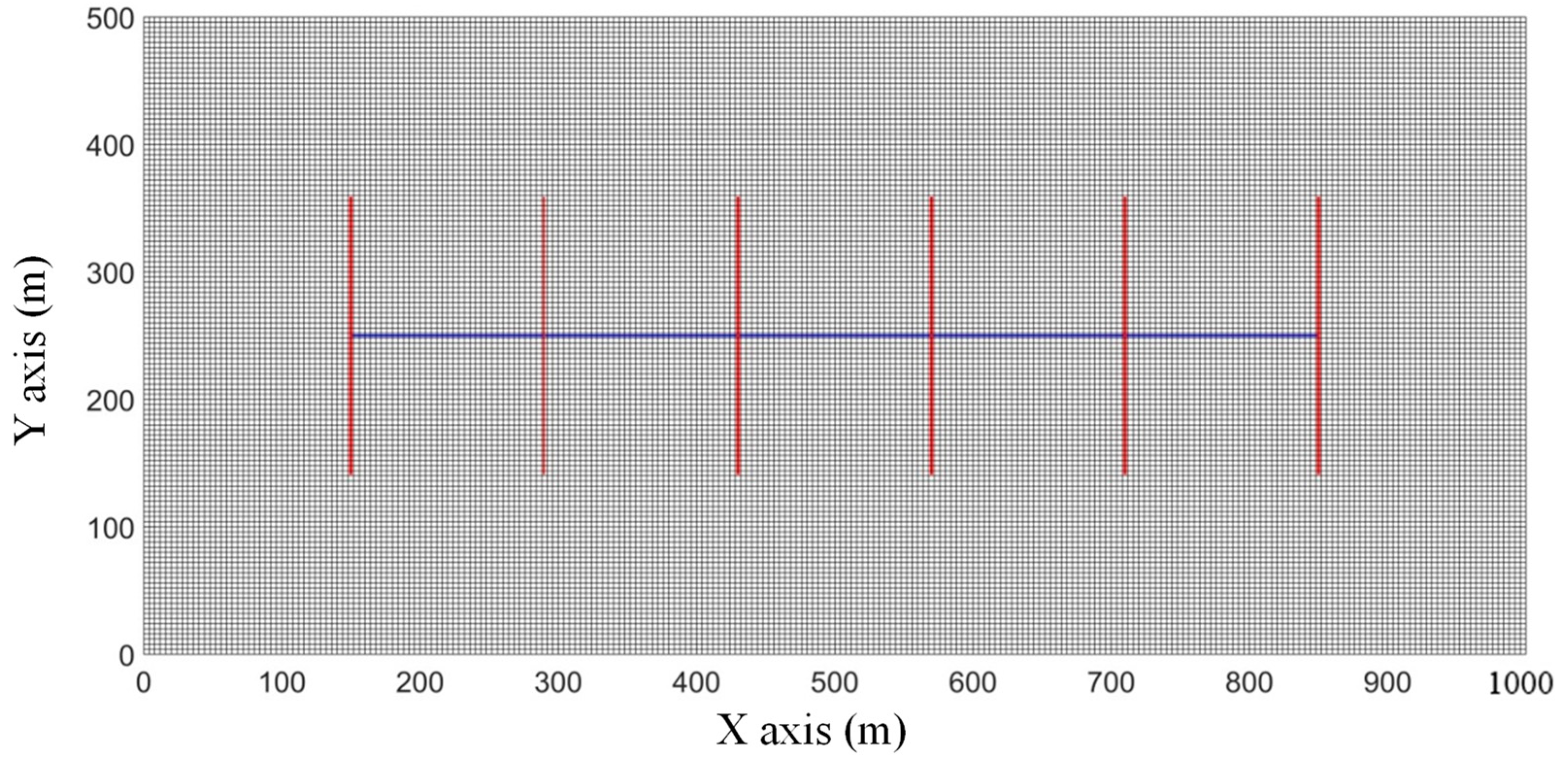
3.1. Numerical Model

The determination of the optimal number of fractures for highly deviated well fracturing is based on a comprehensive evaluation of fracturing well productivity and economic viability. Numerous research findings indicate that an increase in the number of fractures leads to a continuous rise in oil well productivity, although not in a linear manner [32,33,34,35]. As the number of fractures increases, the investment in fracturing also increases, making the implementation of fracturing technology more challenging, and the mutual interference time between production fractures increases. Therefore, the increase in fractures is limited by specific technologies and funds. The optimization of the number of fractures is a crucial research topic for the efficient production of highly deviated well fracturing.

The optimization of fractures is influenced by numerous factors, with the most obvious being the properties of the reservoir and fluids. Furthermore, the number of fractures is influenced by the reservoir’s area and pressure drop. As the permeability of the formation decreases, it could potentially take longer to produce the reservoir until it is depleted, for instance. To expedite the production of the reservoir, it is necessary to create more hydraulic fractures. Furthermore, economic factors play a crucial role as a control factor in determining the ideal number of fractures. The greater the number of fracturing fractures, the more rapidly the return on investment can be realized; however, the optimal number of fractures will result in a higher output/input ratio.

By conducting numerical simulations of productivity in a highly deviated well, considering various numbers of fractures, fracture locations, and fracture geometries in the reservoir, the production capacity and cumulative production output of such wells are established. To maximize fractures, the variables N_f (number of fractures) and Q_Lt (cumulative production) are independent, while the NPV (Net Present Value) is a function of these two. The total investment for highly deviated wells comprise PV₁ (drilling and completion costs), D₁ (fracturing costs for a single fracture), D₂ (conventional production costs), and PV₂ (additional costs). Following the principle of cash flow balance, the NPV of fracturing highly deviated well is given:

$$\begin{gathered} NPV=Q_{Lt}\times \left(P_r-T_a\right)\times S_r\times \left({\frac{P_r}{F\times i_r\times t}}_r\right)-[P{V}_1+D_1\times N_f\times (\frac{P_r}{F\times i_r\times 1}) \\ +P{V}_2\times \left(\frac{P_r}{F\times i_r\times t}\right)+D_2\times \left(\frac{P_r}{F\times i_r\times t}\right)\left)\right] \end{gathered}$$

(18)

where P_r is the crude oil price, dollar/barrel. F is the residual value of funds, dollar. T_a is the oil duty, dollar/barrel. i_r is the discount rate, %. t is the production time, day. PV₁ is the drilling and completion costs, dollar/barrel. D₁ is the fracturing costs for a single fracture, dollar. D₂ is the conventional production costs, dollar. PV₂ is the additional costs, dollar.

By utilizing Equation (18) and combining the results of numerical simulation evaluations of productivity in multi-fractured highly deviated well after fracturing, it is possible to establish the maximum net present value for a highly deviated well with varying numbers of fractures, and thereby determine the optimal number of fractures (Figure 6).

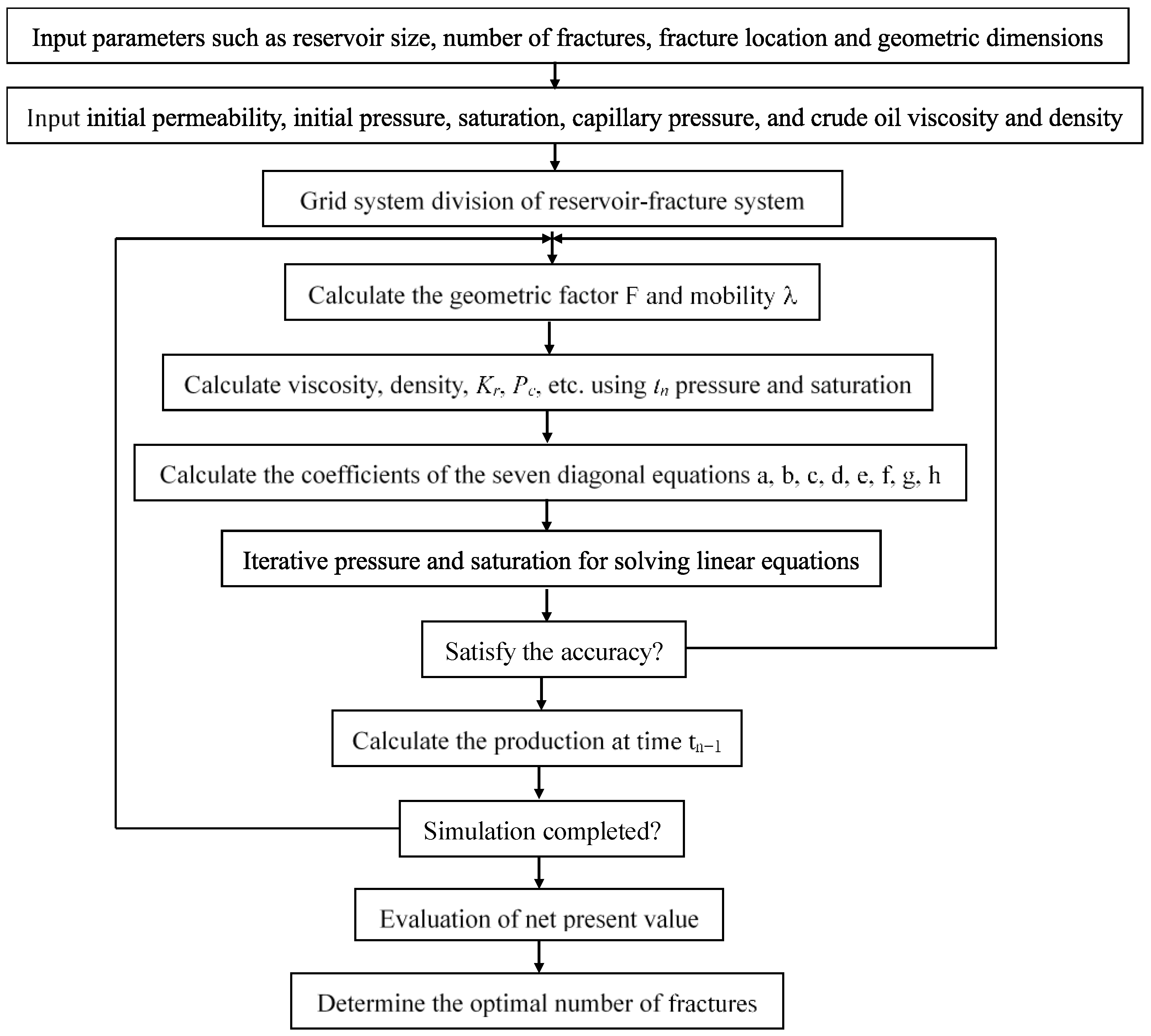
3.2. Mathematical Model Calculation Steps

A numerical simulation model was developed to predict the productivity of multiple fractures in highly deviated wells. A fracture number optimization model was developed, incorporating reservoir grid partitioning and economic evaluation. Based on the research concepts, Figure 7 presents a computational diagram of a numerical simulation model of fracture number optimization for highly deviated wells.

Numerical simulation studies of fracture number optimization in highly deviated wells involve the following main computational steps:

(1)

Enter the geometric dimensions of the reservoir, the number of fractures, the location of fractures, the geometric dimensions of fractures, as well as the physical parameters of the reservoir, including initial permeability, viscosity, density, initial pressure, saturation, and capillary pressure, among others.

(2)

According to Figure 6, divide the reservoir–fracture system grid.

(3)

Calculate the viscosity, density, K_r, P_c, and other parameters at time t_n, and ascertain the coefficients a, b, c, d, e, f, g, and h of the differential Equation (12).

(4)

After solving the seven-diagonal linear equation set, compare it with the initial assumed value, and if it does not meet the accuracy requirement, go back to step (3) and iterate repeatedly until the accuracy requirement is met.

(5)

Calculate the pressure and production at time t_n+1.

(6)

If the time falls short of the development and production time, return to step (3) and continue simulating the production pressure at the subsequent time step until the development and production time is completed.

(7)

Determine the optimal number of fractures for fracturing a highly deviated well by utilizing the fracturing economic evaluation model.

4. Results and Discussion

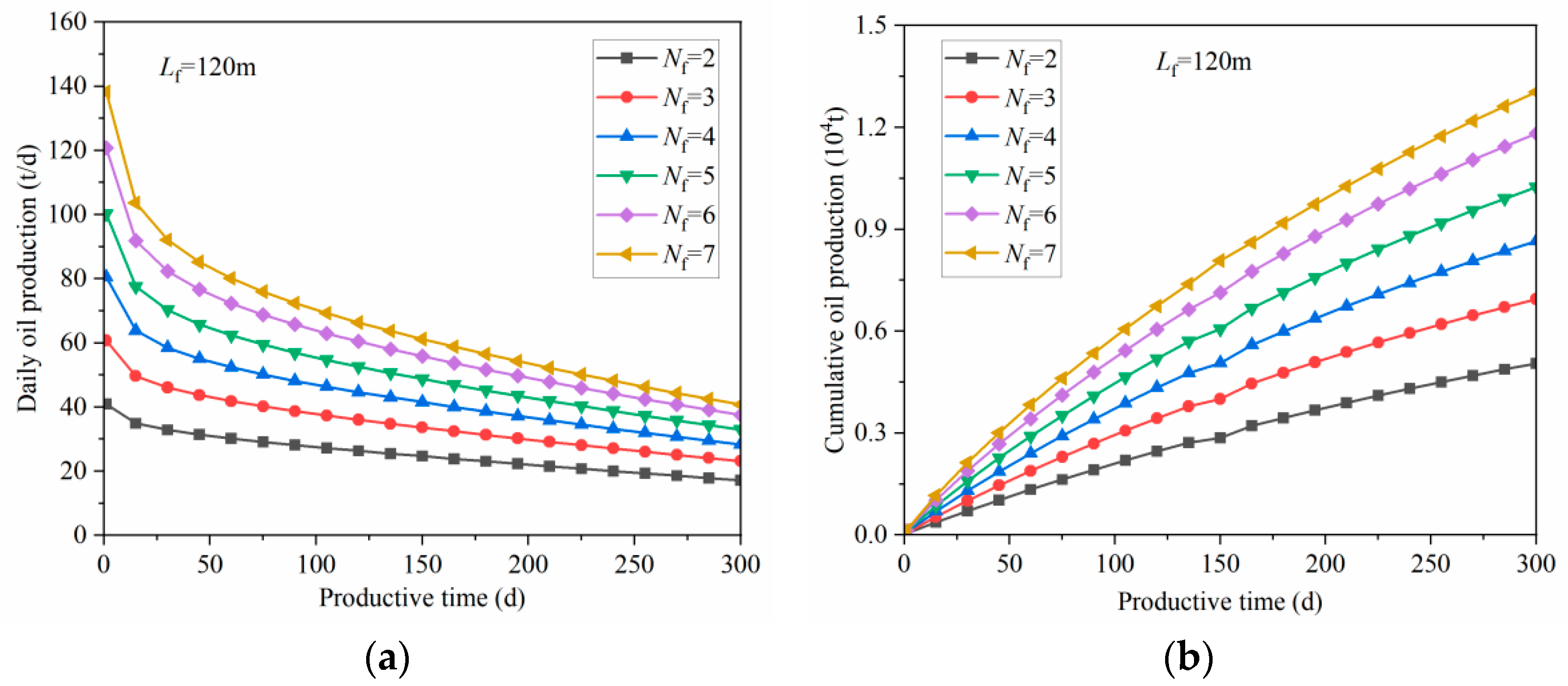
4.1. Case Calculation and Result Analysis

Using the reservoir, fracture, and economic data parameters presented in

Table 1. Reservoir fracture parameters and economic evaluation data.

Parameters	Value	Unit
Reservoir length	1000	m
Reservoir width	500	m
Reservoir thickness	50	m
Porosity	0.10	-
Formation pressure	50.0	MPa
Fracturing cost	0.8	million dollars
Vertical permeability of reservoir	0.01	mD
Horizontal permeability of reservoir	0.1	mD
Fracture permeability	50	mD
Fracture length	50~200	m
Fracture width	0.005	m
Number of fractures	2~7	-
Drilling and completion costs	7.0	million dollars
Oil price	550	dollar/t
Earning rate	0.20	-

, numerical simulations were performed to determine daily and cumulative oil production at various fracture counts, fracture lengths, and permeability rates. Based on the aforementioned model, the productivity of oil wells in the highly deviated reservoir is established for an area of 500 m × 1000 m × 50 m, with an optimal number of six hydraulic fractures, and a reservoir grid size of 4 m × 4 m × 1 m. The grid system is illustrated in Figure 8.

Figure 9, Figure 10, Figure 11 and Figure 12 demonstrate the analysis of the net present value for various numbers of fractures, in conjunction with the fracture economic assessment. In Figure 9, the relationship between single-well oil production and cumulative oil production over various production periods is demonstrated. Both well production and cumulative production increased as the fracture count increased, yet the rate of increase tapered off. Oil well production continued to decline as the year progressed; while total well production may be rising, the rate of increase is gradually decreasing.

The oil production and cumulative oil production curves for wells with varying fracture conductivity are plotted in Figure 10. As the fracture conductivity increases, the production rate of individual wells also increases, and the rate of increase gradually accelerates. As the production time continues, the well production rate decreases, which is more pronounced as the reservoir permeability increases more rapidly.

In Figure 11, curves representing oil production and cumulative oil production are depicted for various numbers of fractures. As the number of fractures increases during the same production period, so does the well’s oil production and cumulative oil production. The longer the production period, the more oil production diminishes and the acceleration of cumulative oil production slows down. The oil production and cumulative oil production curves are depicted in Figure 11 for various fracture lengths. When the number of fractures is kept constant, the cumulative production of the well increases with the fracture length. However, the rate of increase decreased. Production from the well showed a sustained decline as the production time progressed.

The daily and cumulative oil production curves for wells with varying reservoir permeability are depicted in Figure 12. When the number of fractures remains constant, the increase in reservoir permeability results in a marginal boost to daily oil production, which is, however, relatively insignificant. Daily production from the well gradually decreased as production progressed. The effect of a shift in the permeability of the reservoir on the output of the well is not particularly significant.

In Figure 13, the economic net present value curves are presented for various numbers of fractures following well fracturing. As the number of fractures increases, the daily production rate of the well increases, resulting in a higher net present value of the fracture. However, the rate of increase gradually slows. At the same time, as the number of fractures rises, so does the challenge of advancing fracture technology and increasing investment in fracturing. As the number of fractures increases up to a certain level, the net present value of fractures peaks and subsequently decreases. As a result, there exists a specific number of fractures, corresponding to the optimal net present value of the fracture, for a particular fracture technology and financial situation. Based on numerical simulations evaluated for productivity and fracture economics, the appropriate number of fractures is six, and the appropriate fracture length is 200 m, considering the reservoir and fracture parameters.

4.2. Validation of Model Results

The formation pressure nephogram of horizontal wells with varying fracture lengths and a constant conductivity distribution, after 60 days of segmented multi-fracture production, is illustrated in Figure 14. Figure 14 reveals that near fractures with shorter lengths, there’s a noticeable color difference in the formation pressure nephogram, suggesting a rapid decrease in formation pressure. In contrast, near fractures with longer lengths, the color difference diminishes, indicating a slower decrease in formation pressure at that point. This pattern aligns with the behavior observed when considering only a single fracture. After 60 days of production, the formation pressure nephogram shows a pattern dominated by the main fracture, indicating that flow within the reservoir primarily occurs as a Darcy linear flow within the fractures.

In reservoirs with natural fracture systems, the formation pressure at 300 days of segmented multi-fracture production for horizontal wells with the same fracture length and varying fracture conductivity distributions is illustrated in Figure 15. After 300 days of production, the formation pressure has spread to the reservoir boundary, and the formation pressure within the entire reservoir area has begun to decrease, with all pressures below the original formation pressure. As fracture conductivity increases, the decline in formation pressure within the reservoir progressively intensifies, suggesting an expanding flow area controlled by fractures, thereby enhancing the fluidity of the entire reservoir, and promoting the stimulation of oil wells. After 300 days of production, the interference among multiple main fractures intensifies, and the formation pressure distribution begins to exhibit a quasi-radial flow centered on the main fractures.

5. Conclusions

By combining the reservoir–fracture grid system splitting with the IMPES differential method, we have developed a numerical equation for the 3D oil–water two-phase percolation differential for the highly deviated wells. Numerical simulations were performed for various reservoir sizes, fracture locations, and geometrical dimensions, to evaluate the multi-fracture production capacity of the highly deviated wells at different production times, taking into account the inter-fracture interference phenomena at the later stages of post-fracture production. Based on economic assessment models and case calculations of fractures, the number of fractures in the highly deviated wells was optimized, resulting in the following insights:

(1)

A single fracture falls far short of unlocking the full production potential of a highly deviated well. There exists an optimal number of fractures that maximizes production and economic return for such wells. An essential parameter that must be defined prior to fracture design is the optimal number of fractures for the highly deviated wells. Given the complexity of highly deviated wells, it is feasible to employ a three-dimensional oil–water two-phase percolation differential numerical model to simulate the productivity of multiple fractures post-stimulation in such wells.

(2)

The fracturing of highly deviated wells involves multi-fracturing. As production progresses, interference between the fractures appears, affecting fracture production output. Therefore, it is imperative to consider the impact of inter-fracture interference on fracture productivity.

(3)

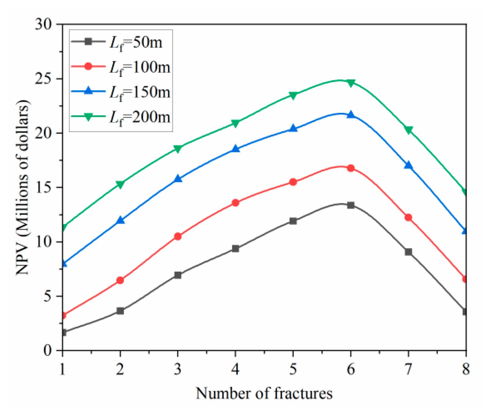
By integrating numerical simulations of post-stimulation multi-fracture productivity with fracturing economic evaluation models, the number of fractures in highly deviated wells can be optimized to six, thereby furnishing a dependable foundation for selecting the scale of fracturing operations and equipment.

(4)

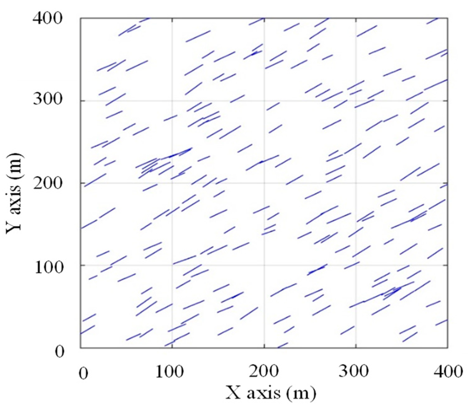
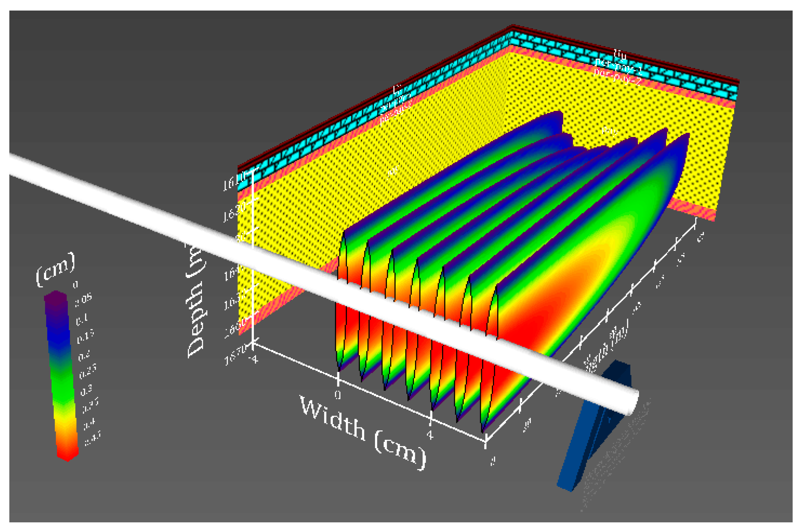
The embedded discrete fracture model establishes a productivity model for fractured wells in oil reservoirs, simulates the performance of oil wells under varying conditions of hydraulic fracture size and conductivity, evaluates the impact of optimizing fracture conductivity on productivity, and takes into account the communication of hydraulic fractures with randomly distributed natural fractures and when six hydraulic fractures are generated by horizontal well fracturing and coexist with natural fractures. The model’s reliability is verified through the post-fracturing strata pressure distribution cloud map.

References

1. Thompson, L.B. Fractured reservoirs: Integration is the key to optimization. J. Pet. Technol. 2000, 52, 52–54. [Google Scholar] [CrossRef]
2. Meyer, B.R.; Bazan, L.W.; Jacot, R.H.; Lattibeaudiere, M.G. Optimization of Multiple Transverse Hydraulic Fractures in Horizontal Wellbores; Society of Petroleum Engineers: Richardson, TX, USA, 2010. [Google Scholar]
3. Song, L.I.; Huiyun, M.A.; Hua, Z.; Jiexiao, Y.E.; Huifen, H. Study on the acid fracturing technology for high-inclination wells and horizontal wells of the sinian system gas reservoir in the Sichuan basin. J. Southwest Pet. Univ. (Sci. Technol. Ed.) 2018, 40, 146. [Google Scholar]
4. Lyu, Z.; Song, X.; Geng, L.; Li, G. Optimization of multilateral well configuration in fractured reservoirs. J. Pet. Sci. Eng. 2019, 172, 1153–1164. [Google Scholar] [CrossRef]
5. Wang, D.; Dong, Y.; Sun, D.; Yu, B. A three-dimensional numerical study of hydraulic fracturing with degradable diverting materials via CZM-based FEM. Eng. Fract. Mech. 2020, 237, 107251. [Google Scholar] [CrossRef]
6. Zhang, N.; Luo, Z.; Chen, X.; Zhao, L.; Zeng, X.; Zhao, M. Investigation of the artificial fracture conductivity of volcanic rocks from permian igneous in the sichuan basin, china, with different stimulation method using an experiment approach. J. Nat. Gas Sci. Eng. 2021, 95, 104234. [Google Scholar] [CrossRef]
7. Chen, M.; Bai, J.; Kang, Y.; Chen, Z.; You, L.; Li, X.; Liu, J.; Zhang, Y. Redistribution of fracturing fluid in shales and its impact on gas transport capacity. J. Nat. Gas Sci. Eng. 2021, 86, 103747. [Google Scholar] [CrossRef]
8. Wang, M.; Wu, W.; Li, S.; Li, T.; Ni, G.; Fu, Y.; Xu, Q. Application and optimization for network-fracture deep acidizing technique of fractured carbonate reservoirs. Lithosphere 2022, 2022, 8685328. [Google Scholar] [CrossRef]
9. Li, S.; Fan, Y.; Yang, J.; Zhao, L.; Ye, J.; Chen, W. Accurate sectional and differential acidizing technique to highly deviated and horizontal wells for low permeable sinian dengying formation in sichuan basin of China. SN Appl. Sci. 2022, 4, 152. [Google Scholar] [CrossRef]
10. Bai, J.; Kang, Y.; Chen, M. Dual effects of retained fracturing fluid on methane diffusion in shale containing adsorbed methane. J. Nat. Gas Sci. Eng. 2023, 110, 204872. [Google Scholar] [CrossRef]
11. Tan, P.; Chen, Z.; Fu, S.; Zhao, Q. Experimental investigation on fracture growth for integrated hydraulic fracturing in multiple gas bearing formations. Geoenergy Sci. Eng. 2023, 231, 212316. [Google Scholar] [CrossRef]
12. Li, S.; Fan, Y.; Wang, Y.; Zhao, Y.; Lv, Z.; Ji, Z.; Min, J. True triaxial physics simulations and process tests of hydraulic fracturing in the Da’anzhai section of the Sichuan Basin tight oil reservoir. Front. Energy Res. 2023, 11, 1267782. [Google Scholar] [CrossRef]
13. Norris, S.O. Predicting oil production from a horizontal well intercepting multiple finite conductivity vertical fracture. SPE Reserv. Eng. 1976, 3, 496–504. [Google Scholar]
14. Karcher, B.J.; Giger, F.M.; Combe, J. Some practical formulas to predict horizontal well behavior. In SPE Annual Technical Conference and Exhibition; OnePetro: Richardson, TX, USA, 1986. [Google Scholar]
15. Soliman, M.Y.; Hunt, J.L.; El Rabaa, A.M. Fracturing aspects of horizontal wells. J. Pet. Technol. 1990, 42, 966–973. [Google Scholar] [CrossRef]
16. Mukherjee, H.; Economides, M.J. A parametric comparison of horizontal and vertical well performance. SPE Form. Eval. 1991, 6, 209–216. [Google Scholar] [CrossRef]
17. Hegre, T.M. Hydraulically fractured horizontal well simulation. In Proceedings of the SPE European 3-D Reservoir Modelling Conference, Stavanger, Norway, 16–17 April 1996; SPE: Richardson, TX, USA, 1996; p. SPE-35506. [Google Scholar]
18. Roberts, B.E.; Van Engen, H.; Van Kruysdijk, C.P.J.W. Productivity of multiply fractured horizontal wells in tight gas reservoirs. In Proceedings of the SPE Offshore Europe Conference and Exhibition, Aberdeen, UK, 3–6 September 1991; SPE: Richardson, TX, USA, 1991; p. SPE-23113. [Google Scholar]
19. Guo, G.; Evans, R.D. Inflow performance of a horizontal well intersecting natural fractures. In Proceedings of the SPE Oklahoma City Oil and Gas Symposium/Production and Operations Symposium, Oklahoma City, OK, USA, 21–23 March 1993; SPE: Richardson, TX, USA, 1993; p. SPE-25501. [Google Scholar]
20. Guo, G.; Evans, R.D. Inflow performance and production forecasting of horizontal wells with multiple hydraulic fractures in low-permeability gas reservoirs. In Proceedings of the SPE Unconventional Resources Conference/Gas Technology Symposium, Calgary, AB, Canada, 18–30 June 1993; SPE: Richardson, TX, USA, 1993; p. SPE-26169. [Google Scholar]
21. Soliman, M.Y.; Hunt, J.L.; Azari, M. Fracturing horizontal wells in gas reservoirs. In Proceedings of the SPE Oklahoma City Oil and Gas Symposium/Production and Operations Symposium, Amarillo, TX, USA, 28–30 April 1996; SPE: Richardson, TX, USA, 1996; p. SPE-35260. [Google Scholar]
22. Raghavan, R.S.; Chen, C.C.; Agarwal, B. An analysis of horizontal wells intercepted by multiple fractures. SPEJ 1997, 2, 235–245. [Google Scholar] [CrossRef]
23. Guo, J.; Gu, F.; Zhou, J. Optimizing the fracture numbers and predicting the production performance of hydraulically fractured horizontal wells. In Proceedings of the PETSOC Annual Technical Meeting, Calgary, AB, Canada, 7–10 June 1997; p. PETSOC-97. [Google Scholar]
24. Roussel, N.P.; Sharma, M.M. Optimizing fracture spacing and sequencing in horizontal-well fracturing. SPE Prod. Oper. 2011, 26, 173–184. [Google Scholar] [CrossRef]
25. Sun, J.; Schechter, D. Optimization-based unstructured meshing algorithms for simulation of hydraulically and naturally fractured reservoirs with variable distribution of fracture aperture, spacing, length, and strike. SPE Reserv. Eval. Eng. 2015, 18, 463–480. [Google Scholar] [CrossRef]
26. Manriquez, A.L.; Sepehrnoori, K.; Cortes, A. A novel approach to quantify reservoir pressure along the horizontal section and to optimize multistage treatments and spacing between hydraulic fractures. J. Pet. Sci. Eng. 2017, 149, 579–590. [Google Scholar] [CrossRef]
27. Taghichian, A.; Hashemalhoseini, H.; Zaman, M.; Yang, Z.Y. Geomechanical optimization of hydraulic fracturing in unconventional reservoirs: A semi-analytical approach. Int. J. Fract. 2018, 213, 107–138. [Google Scholar] [CrossRef]
28. McClure, M.; Kang, C.; Fowler, G. Optimization and design of next-generation geothermal systems created by multistage hydraulic fracturing. In Proceedings of the SPE Hydraulic Fracturing Technology Conference and Exhibition, Muscat, Sultanate of Oman, 11–13 January 2022; OnePetro: Richardson, TX, USA, 2022. [Google Scholar]
29. Lak, M.; Marji, M.F.; Bafghi, A.Y.; Abdollahipour, A. Analytical and numerical modeling of rock blasting operations using a two-dimensional elasto-dynamic Green’s function. Int. J. Rock Mech. Min. Sci. 2019, 114, 208–217. [Google Scholar] [CrossRef]
30. Abdollahipour, A.; Marji, M.F.; Bafghi, A.R.Y.; Gholamnejad, J. Numerical investigation of effect of crack geometrical parameters on hydraulic fracturing process of hydrocarbon reservoirs. J. Min. Environ. 2016, 7, 205–214. [Google Scholar]
31. Lak, M.; Marji, M.F.; Bafghi, A.R.Y. Discrete element modeling of explosion-induced fracture extension in jointed rock masses. J. Min. Environ. 2019, 10, 125–138. [Google Scholar]
32. Bazan, L.W.; Brinzer, B.C.; Meyer, B.R.; Brown, E.K. Key parameters affecting successful hydraulic fracture design and optimized production in unconventional wells. In Proceedings of the SPE Eastern Regional Meeting, Pittsburgh, PA, USA, 20–22 August 2013. [Google Scholar]
33. Kim, K.; Ju, S.; Ahn, J.; Shin, H.; Shin, C.; Choe, J. Determination of key parameters and hydraulic fracture design for shale gas productions. In Proceedings of the International Ocean and Polar Engineering Conference, Big Island, HI, USA, 22–26 June 2015. [Google Scholar]
34. Zheng, S.; Sharma, M.M. Evaluating different energized fracturing fluids using an integrated equation-of-state compositional hydraulic fracturing and reservoir simulator. J. Pet. Explor. Prod. Technol. 2022, 12, 851–869. [Google Scholar] [CrossRef]
35. Kang, C.A.; McClure, M.W.; Reddy, S.; Naidenova, M.; Tyankov, Z. Optimizing shale economics with an integrated hydraulic fracturing and reservoir simulator and a Bayesian automated history matching and optimization algorithm. In Proceedings of the SPE Hydraulic Fracturing Technology Conference, The Woodlands, TX, USA, 1–3 February 2022. [Google Scholar]
Figure 1. Physical model of highly deviated wellbore fracture.
Processes 12 00179 g001
Figure 2. Planar model of reservoir grid with fracture.
Processes 12 00179 g002
Figure 3. Embedded discrete fracture model with random distribution of natural fractures.
Processes 12 00179 g003
Figure 4. High-angle well reservoir fracture wellbore profile.
Processes 12 00179 g004
Figure 5. Grid diagram of fractured reservoir–fracture system.
Processes 12 00179 g005
Figure 6. Numerical simulation of multi-slit fracturing in highly deviated wells.
Processes 12 00179 g006
Figure 7. Numerical simulation calculation diagram for optimizing the number of fractures.
Processes 12 00179 g007
Figure 8. Reservoir grid system with six fractures.
Processes 12 00179 g008
Figure 9. Oil production and cumulative production curves under different production times. (a) Daily production. (b) Cumulative production.
Processes 12 00179 g009
Figure 10. Oil production and cumulative production curves under different fracture diversion capacities. (a) Daily production. (b) Cumulative production.
Processes 12 00179 g010
Figure 11. Oil production and cumulative production curves under different fracture lengths. (a) Daily production. (b) Cumulative production.
Processes 12 00179 g011
Figure 12. Oil production and cumulative oil production curves under different formation permeability. (a) Daily production. (b) Cumulative production.
Processes 12 00179 g012
Figure 13. Curve of the net present value of oil well production and the number of fractures under different fracture lengths.
Processes 12 00179 g013
Figure 14. Cloud chart of formation pressure distribution at 60 days of production under different fracture lengths (without natural fractures). (a) The fracture length is 100 m, and the conductivity is 50 mD·m. (b) The fracture length is 150 m, and the conductivity is 50 mD·m.
Processes 12 00179 g014
Figure 15. Cloud chart of formation pressure distribution at 300 days of production under different fracture lengths (with natural fractures). (a) The fracture length is 150 m, and the conductivity is 50 mD·m. (b) The fracture length is 150 m, and the conductivity is 100 mD·m.
Processes 12 00179 g015