1. Introduction
It is important to investigate the flow field in axial pumps [
1,
2]. The outflow quality control of circulation pumps is the main consideration in determining the technical details of a circulation flow system [
3,
4]. To investigate the characteristics of unsteady flow within pumps, it is necessary to conduct an effective analysis of the pumps’ efficiency [
4,
5]. In the study of the pattern of internal flow in axial pumps through varying flow operations, common methods include complex 3D unsteady flows, frequently involving multifaceted flow fields and high levels of pulsation, pressure, acoustics, and noise [
6,
7]. To analyse the characteristics of the internal flow inside axial pumps under changing geometrical conditions and parameters, it is necessary to suppress the pressure pulsation, noise, and acoustic levels within the pumps [
8]. Presently, numerical investigation using computational fluid dynamics (CFD) is a powerful technique used to study the structure of the flow field within pumps. In combination with experimental design techniques, it has been employed to analyse the multifaceted flow behaviour within axial pumps. Many researchers have conducted wide-ranging studies on the 3D flow patterns and pulsations in pressure within flow pumps. Wang et al. [
9] performed both experimental verification and computational calculations to indicate the development of the characteristics of a skewed flow within an S-shaped system of fifteen degrees in an axial pump. Kim et al. [
10] studied the unsteady and steady performance of a type of submersible axial pump based on the inner guide blades and the angle of the blade pitch. Zuo et al. [
11] investigated the impact of varying pump speeds on the characteristics of the unsteady inner and external flow in axial pumps by combining computational and experimental tests. AI-Obaidi et al. [
12] studied the different pressure, tangential, axial, and radial velocities, in addition to the fluctuating pressure within the axial pump, according to the k-epsilon turbulence model and using sliding mesh technology. Kang et al. [
13] noted that increasing the number of guide blades could enhance the axial velocity uniformity within the outlet of the impeller, through computational calculations of the inner patterns in the axial pump. Xie et al. [
14] discussed the importance the characteristics of the pressure fluctuations within a model pump, using a prototype pump developed with CFD and an experimental setup, suggesting that predictions and numerical calculations could replace experimental testing with a pressure pulsation model.
Zhang et al. [
15] analysed the characteristics of unsteady turbulence with the interaction of the fluid flow structural characteristics in a vertical axial pump under flow design conditions. They revealed the time frequency of pulsations in fluid pressure and the pattern of acoustics with similar positions within an axial pump. Mu et al. [
16] tested the groove flow control of axial pumps. A numerical technique was applied to investigate the characteristics of the pump’s internal flow and then the results were enhanced with stall flow conditions. Kang et al. [
17] enhanced the characteristics of the inner flow in an axial pump under low-water conditions by adopting a structure of two pipe inlets and combining experimental techniques with numerical calculations.
Kan et al. [
18] numerically applied the k-omega turbulence model to simulate the helical axial pump type. The effect of the clearance area between the casing and blade tip region on the characteristics of the internal flow was observed through investigating the pressure streamline in the pump and TKE. Yang et al. [
19,
20] analysed the characteristics of the pressure pulsation and internal flow within the guide blades and impeller in a vertical axial pump by applying varying flow conditions, and they investigated the characteristics of the inner flow near the inlet and outlet at different deflection angles according to the k-omega turbulence model. They observed that the outer flow velocity was uniform and the pulsation in pressure was periodic with an increase in the deflection blade angle. Feng et al. and Al-Obaidi et al. [
21,
22] applied computational methods to assess the impact of the clearance area between the pump casing and blade tip on fluctuations in pressure in an axial pump; they then proposed a new technique depending on the variations in the pressure statistics to calculate the fluctuation in pressure of the entirety of the grid nodes for all pumps.
In addition, it has been noted that there exist multifaceted vortex structures within pumps, and these vortices in the flow are a significant aspect that causes pulsations in pressure within axial pumps, hence garnering important attention in the flow domain [
23]. Zhao et al. [
24] investigated the corner vortex characteristics in mixing, separated, and secondary flows in axial pumps and observed that the turbulent vortex dissipation and vortex strength progressively weakened along the line of the vortex core area to the vortex tail area under varying water flow conditions. Zhang et al. [
25] considered the impact of the inner flow vortex on axial pump device performance under changed water conditions, with the use of computational calculations as well as experimental testing. It was noted that the change in the type of internal vortex in an impeller blade and pulsations in pressure were caused by these vortex flows. Kan et al. [
26] employed numerical code to analyse the flow type steady state conditions; then, they investigated the characteristics of an unsteady flow in an axial pump at stall flow conditions, observing that a low frequency in the pressure pulsation mechanism occurred at stall flow conditions. In addition, they investigated the evolution and position of the core flow zone of the guide blade vortex pattern at deep stall flow operations. Song et al. [
27] calculated the impact of attached flow vortices on pulsations in the pressure of the pump by combining experimental tests and vortex flow dynamics conditions. It was noted that the pulsation in pressure occurred through the attached flow vortices periodically along with time, and the curve of the pressure pulsation was roughly a type of cosine curve.
Wu et al. [
28] applied the technology of PIV flow testing to obtain the characteristics of the unsteady state conditions of a leakage vortex with the clearance of the impeller blade tip in an axial pump at varying water conditions; then, they investigated the fragmentation separation and generation procedure of the leakage flow vortex.
According to the various investigation results stated above, the analysis of the characteristics of flow within axial pumps mostly focuses on the characteristics of the pressure pulsation and the distinctive vortex flow inside an impeller interference area. However, the investigation of the flow and vortex evolution in the pump is comparatively lacking, and the influence of the inner flow is yet to be revealed. As mentioned above, there are few investigations and analyses of the hydraulic performance and dynamic characteristics of pumps using both CFD and acoustic techniques based on numerical calculations and acoustic tests. Consequently, a targeted investigation is urgently required. In this research, numerical simulation and acoustic methods are used to experimentally and numerically simulate the 3D structure of the unsteady flow of a circulation axial pump with varying water rates, as well as the unstable flow evolution region on the surface of the blade. Moreover, the development and evolution laws of the structure of the internal vortex are studied, and a qualitative and quantitative investigation of the pump via flow uniformity indicators is performed in detail.
5. Results and Discussion
5.1. Experimental Results
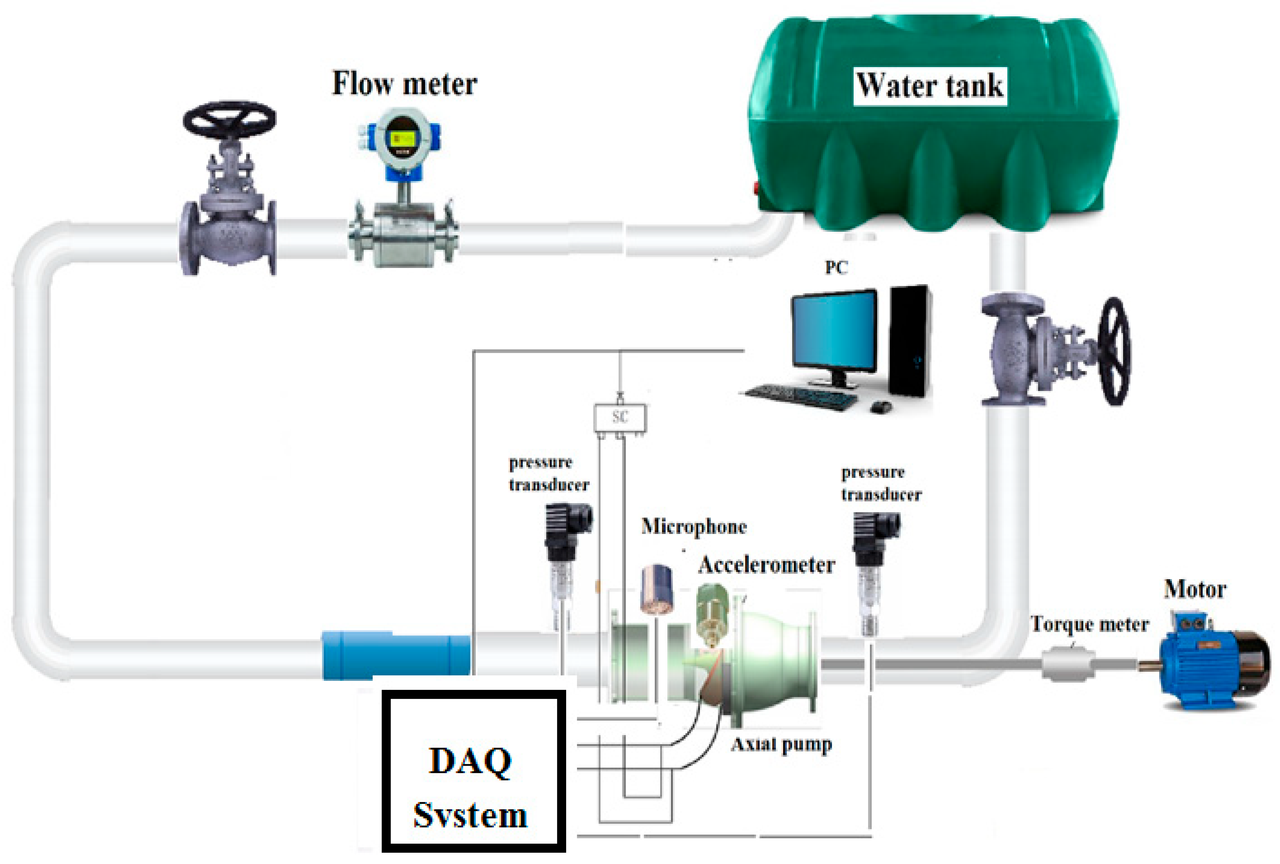
In order to analyse the various flow conditions involved in the pump’s performance, experimental data were collected for the pressure at both the suction and discharge parts, as well as the acoustic signals.
5.2. Investigation of Pressure in Axial Pump Based on Time Domain
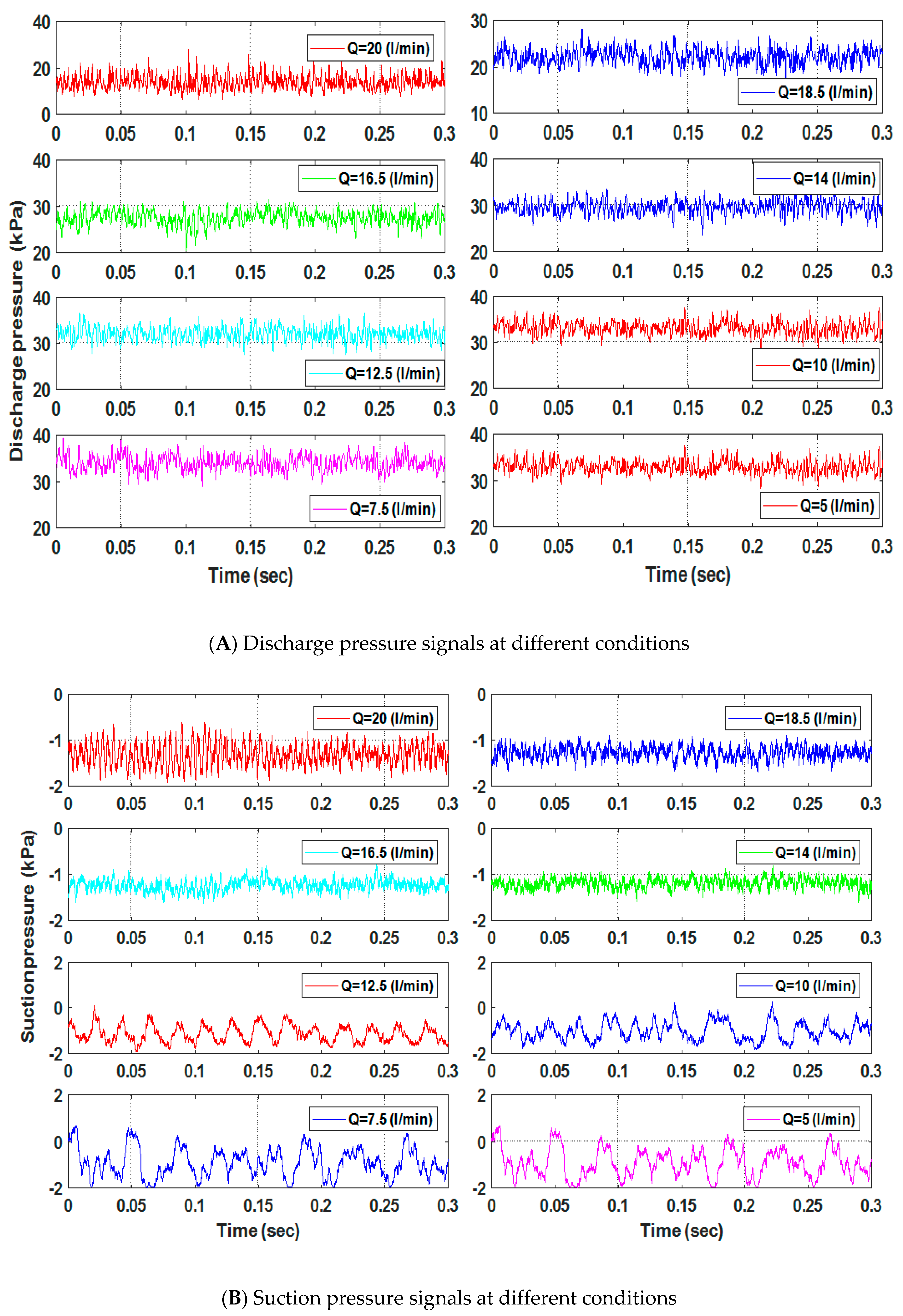
The axial pump’s instantaneous suction and discharge pressures are shown in the time domain in
Figure 7, for various water flows between 5 and 20 (L/min) at a speed of 3000 rpm. These statistics show that as the water flow in the pump changes, the pressure signals at both suction and discharge follow the same trend. Additionally, when the trend of flow increases, the trend of the pressure signal magnitude decreases. This occurs as a result of the effects of hydraulic loss and mechanical loss on the pump, as well as more mixing, secondary flow, and tip leakage vortices that occur in the impeller’s suction. All of these factors contribute to a more unstable flow in the axial flow pump. However, the time domain shift in the pressure signal does not provide a good indication of how the performance of the pump varies. As a result, further analysis is required to determine the impact of different water flow rates in the pump on the pressure signal, utilising a range of features, as described in the next section.
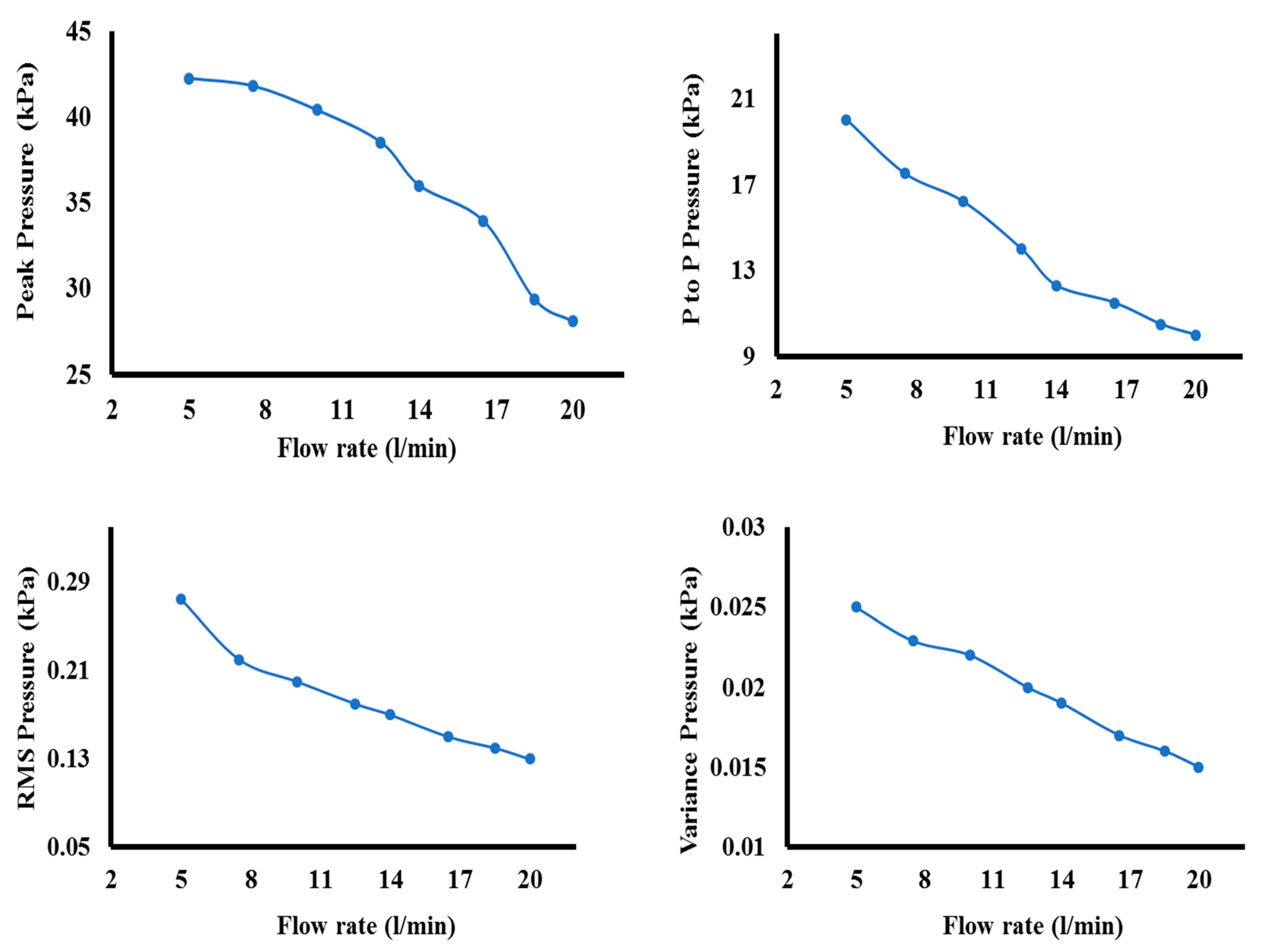
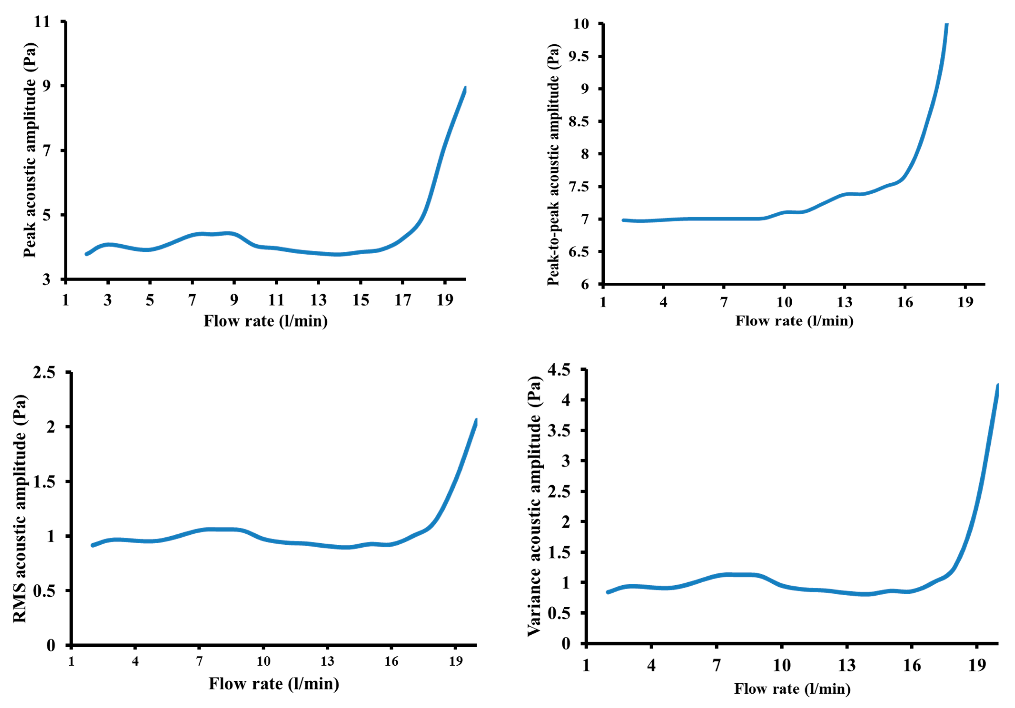
As indicated in the previous section, examining pressure signals only in the time domain does not give a clear picture of how the flow affects the pressure signals.
Figure 8 shows the application of several statistical features for pressure signals with varying flows between 5 and 20 (L/min) at a starting speed of 3000 rpm, including peak, peak-to-peak, RMS, and variance features. It is discovered that all of these characteristics have a roughly identical tendency, continuing to decline as the flow conditions increase. This is due to cavitation, which occurs most frequently under high-flow circumstances and high-flow interactions between flows that are caused by the axial impeller and pump casing. As already indicated, while the pump is operating under more mixing, secondary flow, and tip leakage vortices, very small bubbles begin to form and disintegrate. Due to these bubbles collapsing, the pump’s impeller will vibrate more loudly and generate more noise.
5.3. Investigation of the Acoustic Signals in Axial Pump Based on Time Domain
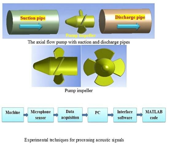
In this study, an acoustic approach was used to analyse the flow fluid behaviour in the axial pump under various experimental conditions and noise levels. Three readings were recorded for each of the test situations to guarantee the reliability and reproducibility of the results. Different sets of features for the detection of the flow pattern in the acoustic data were found using the analysis of signals by the MATLAB code. These immediate acoustic impulses underwent temporal and frequency domain analysis. This research made it possible to forecast pump cavitation. For the time domain analysis, several statistical features were used, and for the frequency domain, the FFT approach was used with various frequency ranges.
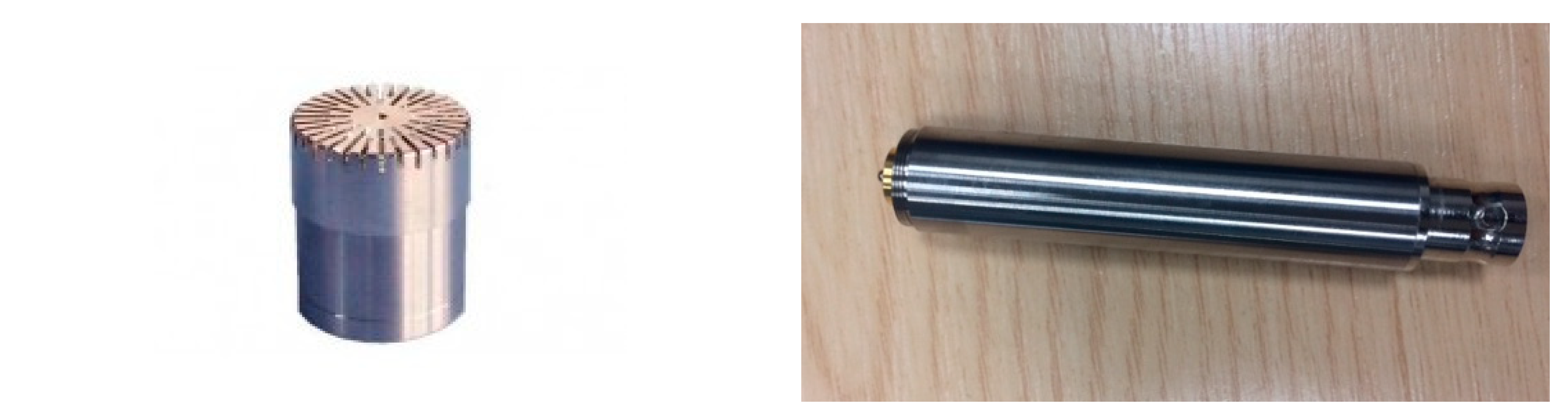
In this study, acoustic signals were collected using a microphone, whereas the flow rate was measured utilising a water flow meter. The amplitude of the aforementioned signals differs with time in the temporal domain. A relationship between the induced flow and the acoustic signal from the axial pump has been established as a result of the analysis of the experimental data, which reveals a trend in the features caused by acoustic signals with variations in flow rate.
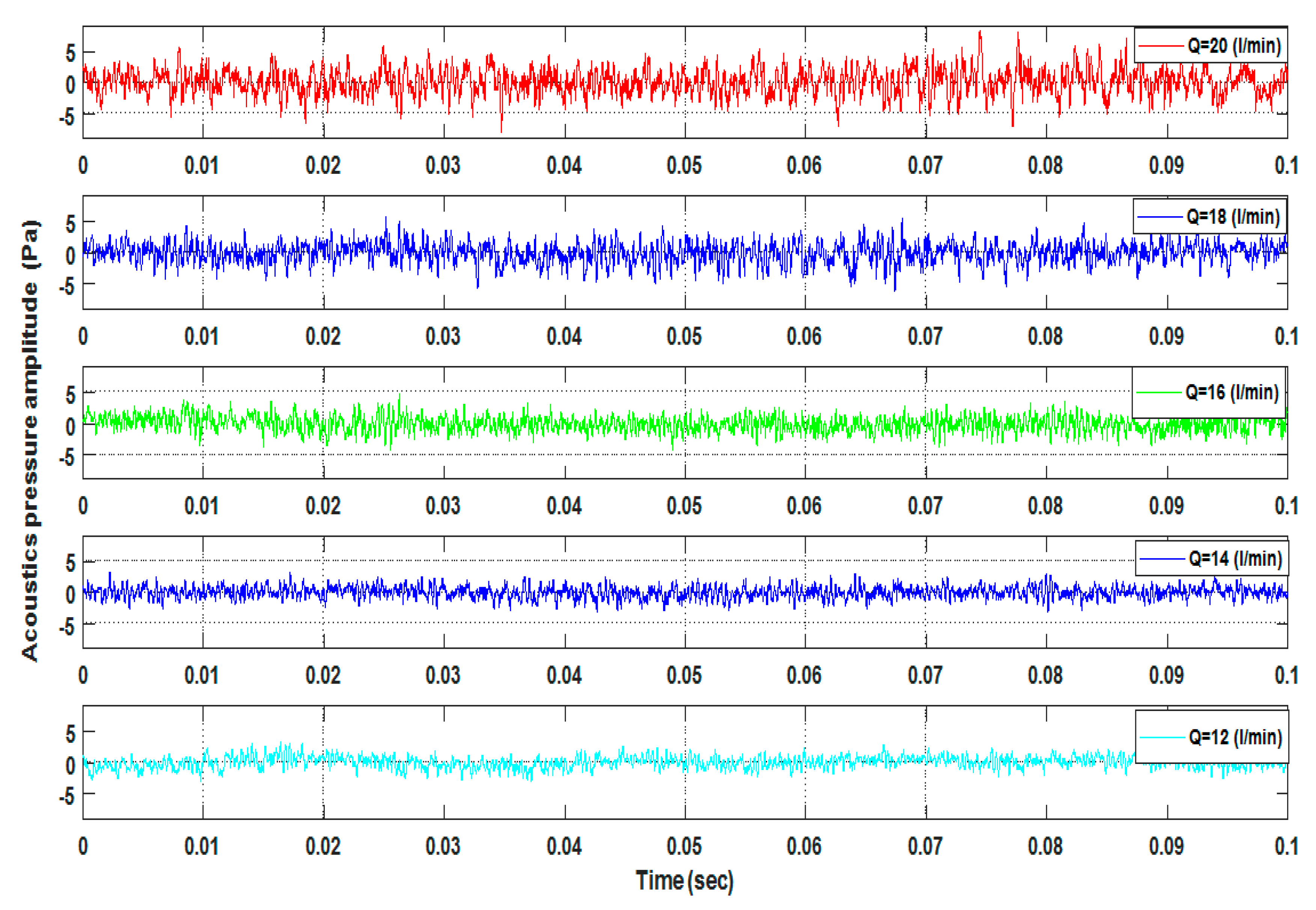
Figure 9 shows the time wave shapes for the analysis of the acoustic signals with various flows at a 3000 rpm rotation speed. It is clear that the properties of the acoustic signals remain mostly unchanged when the flow is less than the design flow of 15 L/min. It is evident that there is a substantial change in the forms and amplitudes of the acoustic waves at high flow rates greater than 16 L/min. These alterations in the acoustic signal could be caused by one of two factors. The first is a result of the intense engagement between the volute and impeller. The second, as discussed in the previous section, is due to the onset of more mixing, secondary flow, and tip leakage vortices in the pump, which leads to a greater NPSHR value than the NPSHA at high flow. These values can be compared to show that acoustic signals are capable of detecting more mixing, secondary flow, and tip leakage vortices within a pump.
Figure 10 shows the analysis of the data from the pump’s acoustic waveforms employing features under various operational settings ranging from 5 to 20 L/min. As seen in the figure, there were several variations in the acoustic signals at various flow conditions. However, the level of the acoustic signal showed a notable increase at flow values more than 15 L/min. The results presented the same tendency for all of the features that correlated with the acoustic signals under altered flow circumstances. It has been discovered that all the statistical parameters quickly increase when the axial pump operates at a flow rate greater than 16 L/min. The main causes are the aforementioned factors, as well as the vortex. Pump flow instabilities are caused by the strength and vorticity of the flow, large pressure variations inside the pump, and high flow conditions. As a result, the collapse of these bubbles will result in increased noise and acoustics in the pump’s impeller.
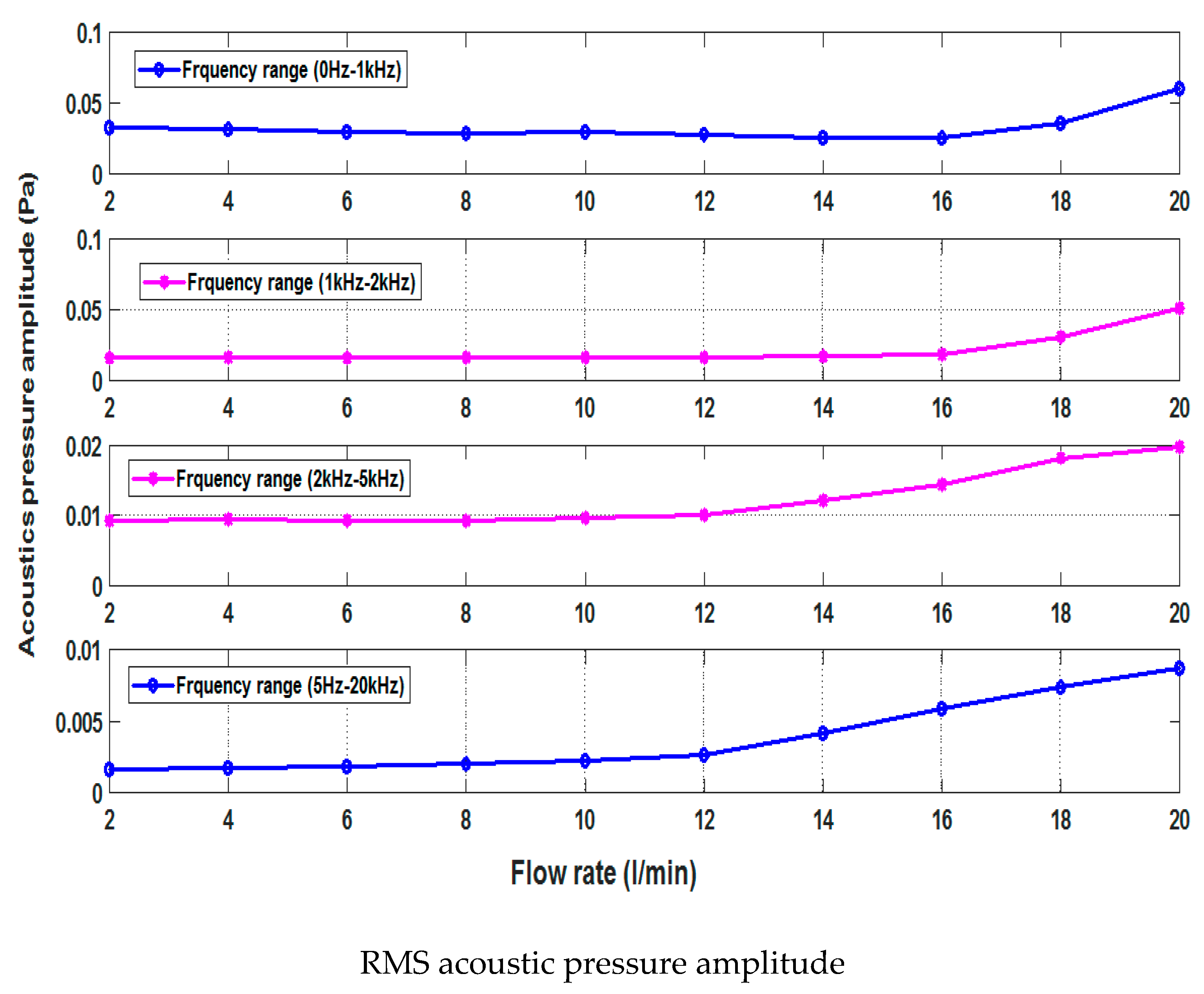
5.4. Investigation of the Acoustic and Pressure Signals in Axial Pump Based on Frequency Domain
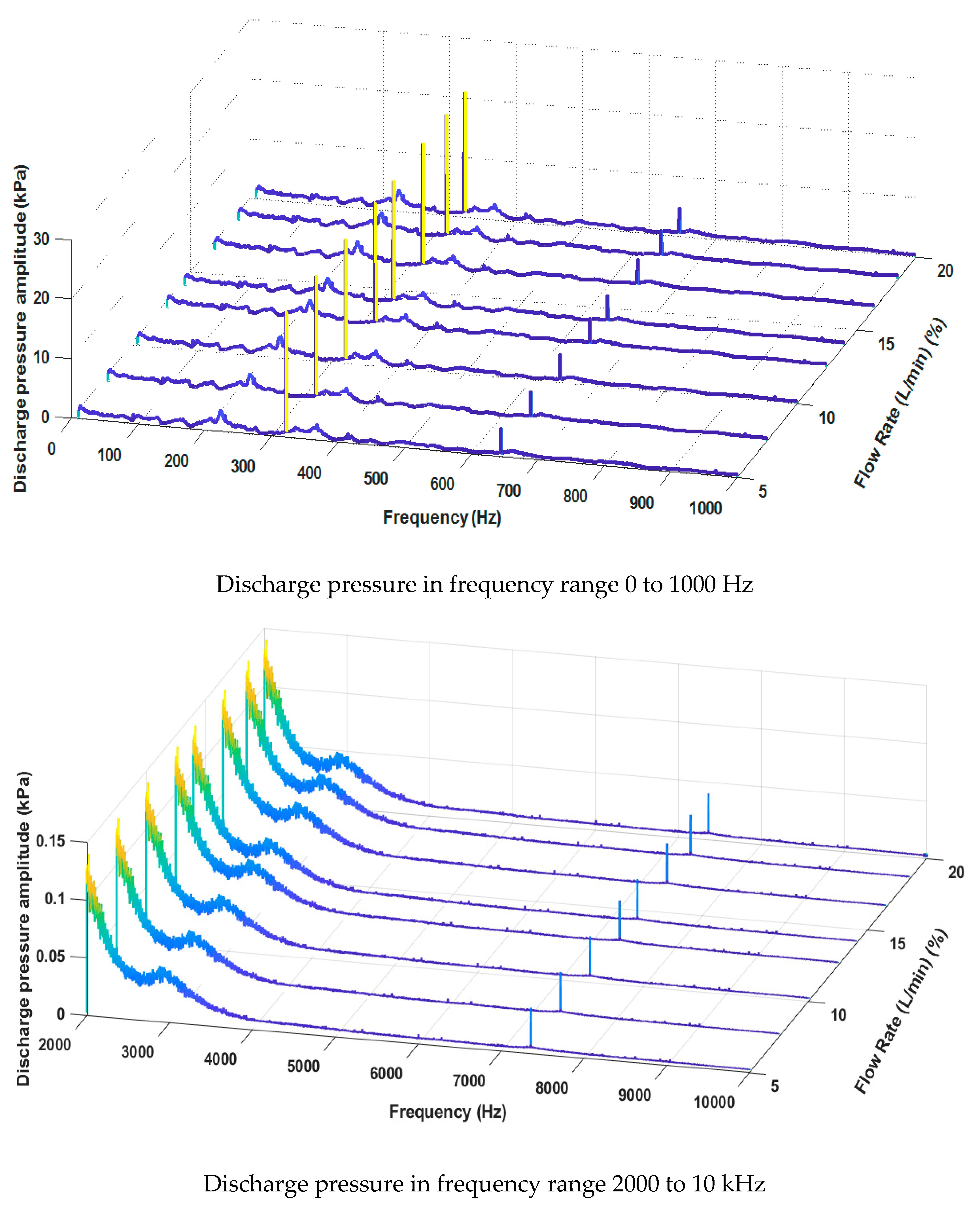
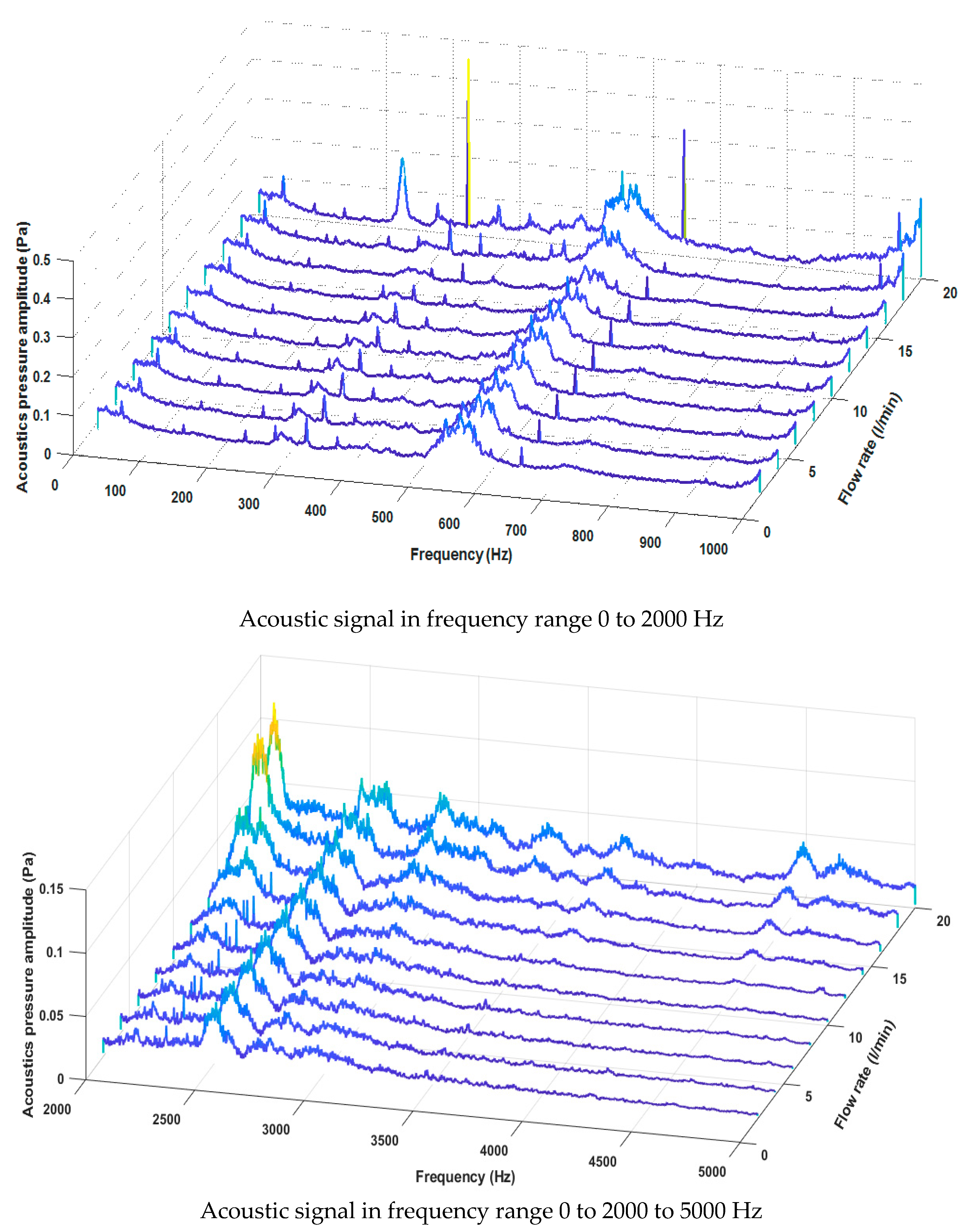
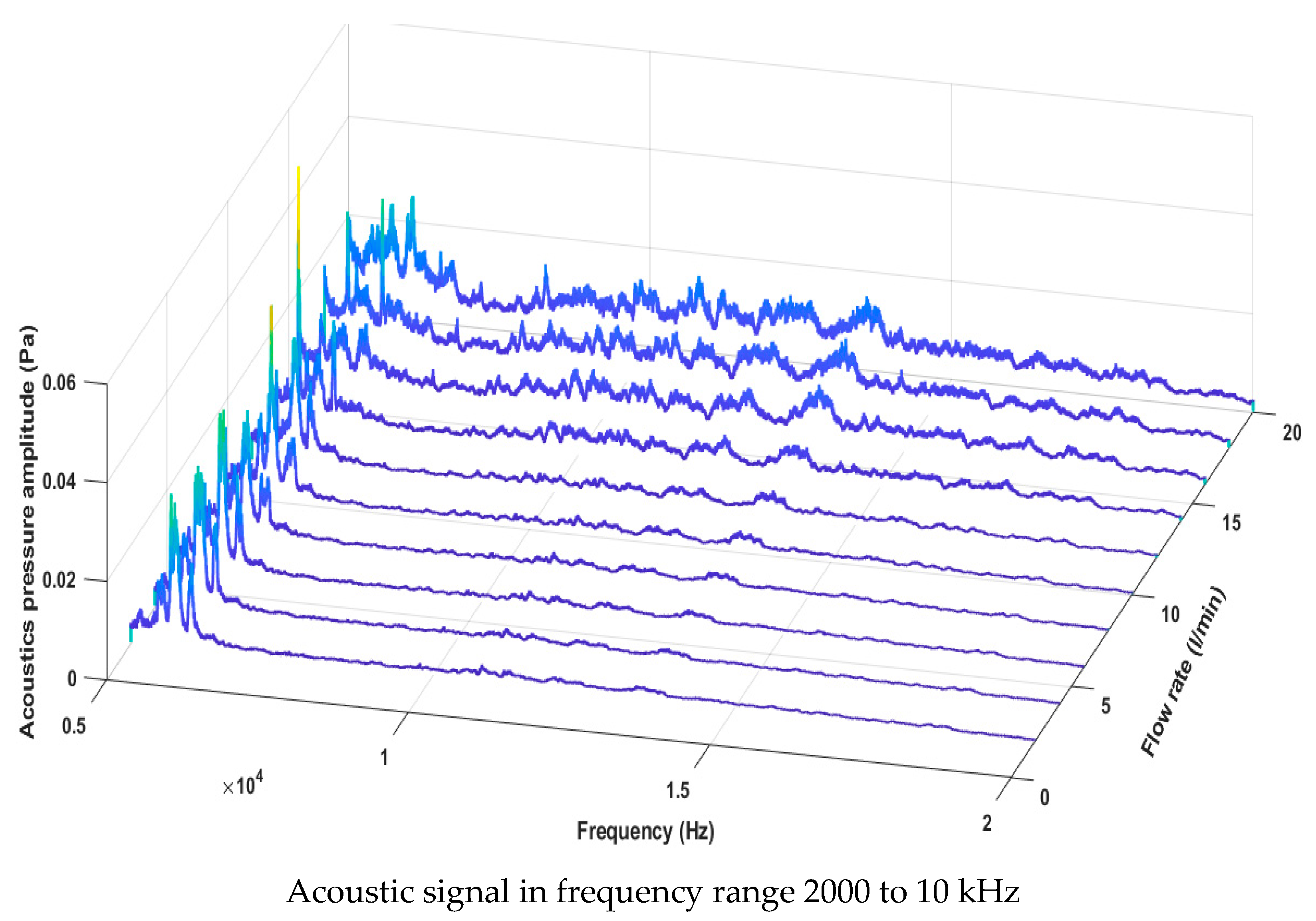
The 3D signals obtained in the frequency study according to various frequency ranges are shown in
Figure 11. The first range of frequencies was from 0 Hz to 1 kHz, and, at various flow and pump speeds, such as 3000 rpm, the second range of frequencies was from 2 kHz to 20 kHz, with various acoustic signals. Depending on these values, there are variations in the axial pump’s pressure and acoustic level amplitudes. However, it is clear that the amplitude was altered and increased as the axial pump operated at larger flow rates for both frequency ranges. We have established that the pressure frequency range and the pump’s acoustic frequency range exhibit similar characteristics. The vortex was the major contributing factor. A strong and vorticious flow, significant interactions between the water and pump components, the onset of more mixing, secondary flow, and tip leakage vortices occurrence, and more random flows with higher peak counts than in low-flow circumstances are all factors. The dominant frequencies in each of these frequency bands were related to the BPF of the rotating shaft pump and its harmonics. Therefore, a frequency analysis of the pressure and acoustic signal in the axial pump can provide a useful indicator for the pump. Consequently, methods of monitoring pumps utilising sensors, such as pressure transducers with accelerometers, may be used to diagnose and identify the flow field structure in various scenarios, such as a normal flow, instable flow, or more mixing, secondary flow, and tip leakage vortex conditions.
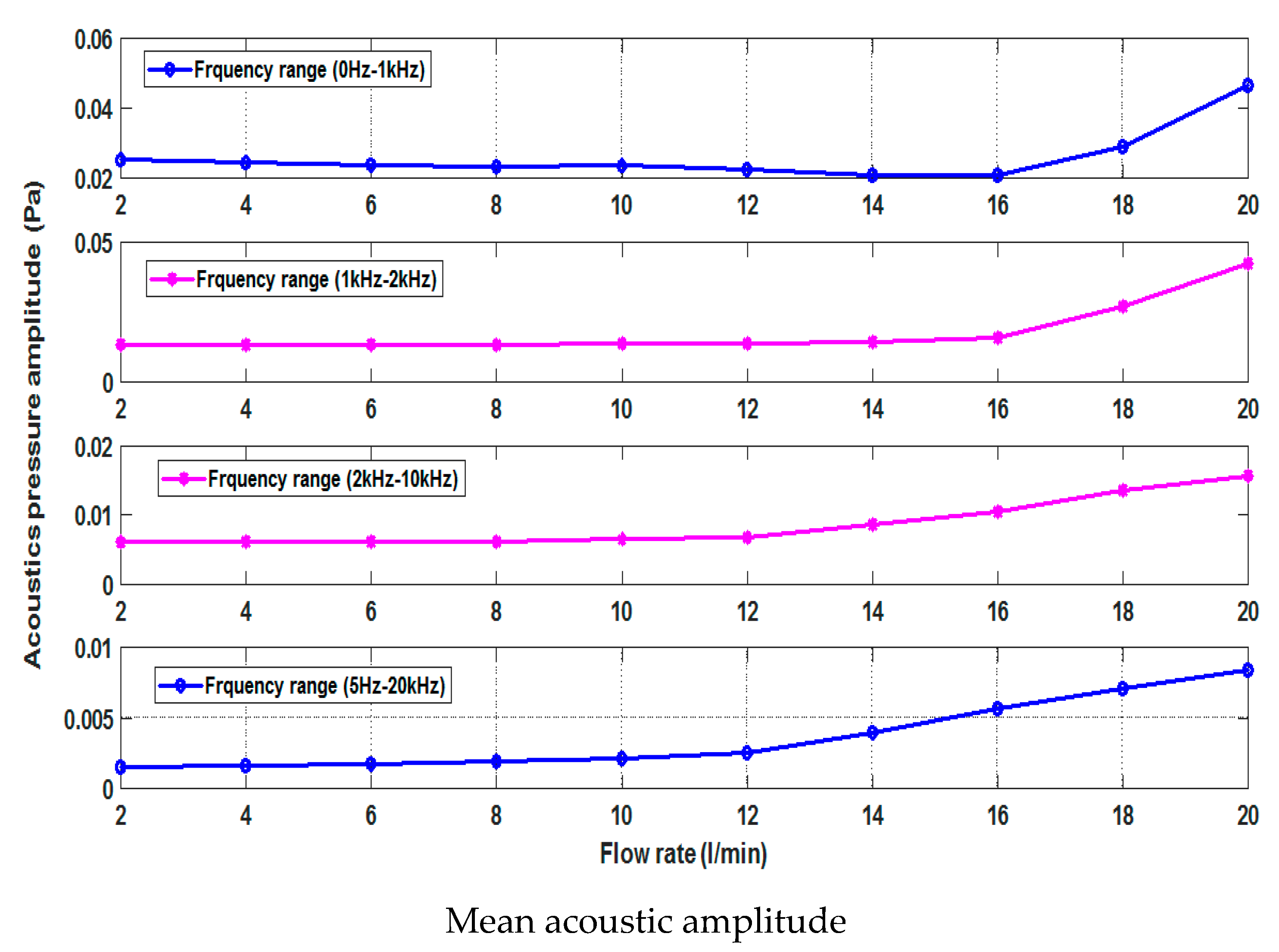
Figure 12 displays both the mean and RMS values of the signals in the frequency domain for various flow rates and N = 3000 rpm under different frequency ranges from 0 to 20 kHz. When the pump runs at a flow lower than 16 L/min, there is no appreciable change in the mean acoustic amplitude value. However, it is evident that more mixing, secondary flow, and tip leakage vortices cause the level of the acoustic amplitude to rapidly grow at a flow rate greater than 16 L/min. Because of the high flow rate, the NPSHR is higher than the value of the NPSHA.
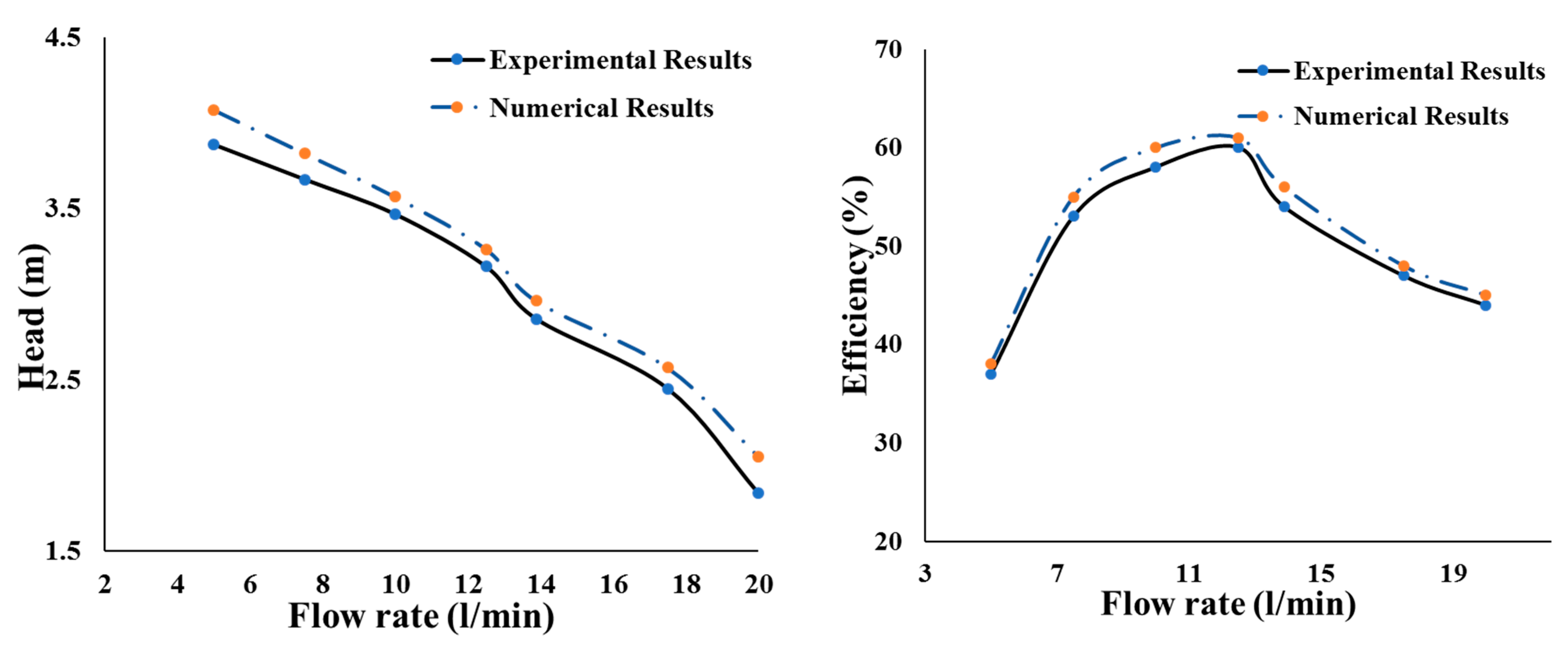
5.5. Performance of Hydraulic Systems
Using a steady state computation, the pump head H was determined. The mesh and turbulence models were found to be applicable by comparison with the external characteristics experiment. In
Figure 10, the predicted error is less than 7.5% when compared to the experimental data. Transients were computed using the QBEP under typical operational conditions. The results of the numerical simulations mirrored the experimental findings, as seen in
Figure 13. In this study, axial flow pump models were investigated. The head and efficiency curves of the pump were then calculated at a speed of 3000 r/min. In
Figure 10, these comparisons are represented. The axial flow pump validation data in the experimental and numerical results for efficiency and head at the design flow condition of 7.5 and 6.5 percent, respectively, were obtained according to the numerical simulation. The head and efficiency curves in the numerical simulation were remarkably comparable to those found in the experiments, demonstrating the accuracy and applicability of the method.
The head is calculated using the formula below:
is the measurement of the volumetric section in the inner pressure and is the volumetric section in the outlet pressure as well as the total pressure.
The following formula is used to determine the hydraulic efficiency:
where
Tp represents torque, N·m.
Undoubtedly, measurements play a major role in many applications, such as establishing scientific truths, tracking system activity, and communicating technical specifics. As a result, all industries incur significant costs in acquiring and maintaining measurements from various types of test apparatus. In any test measurement technique, the measurements need to be as precise as possible and must be thoroughly examined. Finding the physical quantity to be measured is the first step in any analysis of the uncertainty of measurement.
The standard deviation
σx of the sampled data was used in this study’s calculation of the uncertainty measurement using the equation below:
The following equation was used to compute mean value’s uncertainty:
Next, we determine the signal’s mean value:
The mean value of uncertainty can be computed using the above method, as indicated in
Table 4 which summarises the mean values of uncertainty for the various sensors employed in this experimental investigation.
5.6. Vortex Core Trajectory and Tip Clearance Flow Structure
Structure of the Gap Flow Vortex
For various flow rates (between 5 and 20 L/min),
Figure 14 shows the pressure variations along with clearance leakage flow patterns and vortex distributions. The clearance flow is depicted in this figure moving through the gap from the pressure surface to the suction surface. Large vortices are present throughout the suction surface. The leakage flow travels lengthwise in addition to circumferentially. As the chord is lengthened, the rate of leakage is reduced. The isosurface reflects the streamlines of the spiral structure as a result of the vortex structure. There is an extended vortex structure on the proximal blade. In
Figure 8, a clockwise-revolving induced vortex is depicted. This vortex structure was created artificially. Tip separation vortices also covered a sizable portion of the blade’s tip.
The interactions between the vortex and secondary flow resulted in the local appearance of a tip leakage vortex structure. A second tip leakage vortex also developed downstream and in the centre of the blade. The distribution of vorticity along the transverse sections is depicted in
Figure 15. This was a result of the high vorticity that was present close to the gap’s exit. Because the leakage flow left the gap at a high flow rate, shear layers formed quickly between the main flow and the leakage flow. Near the end wall, there was a negative-vorticity-induced vortex.
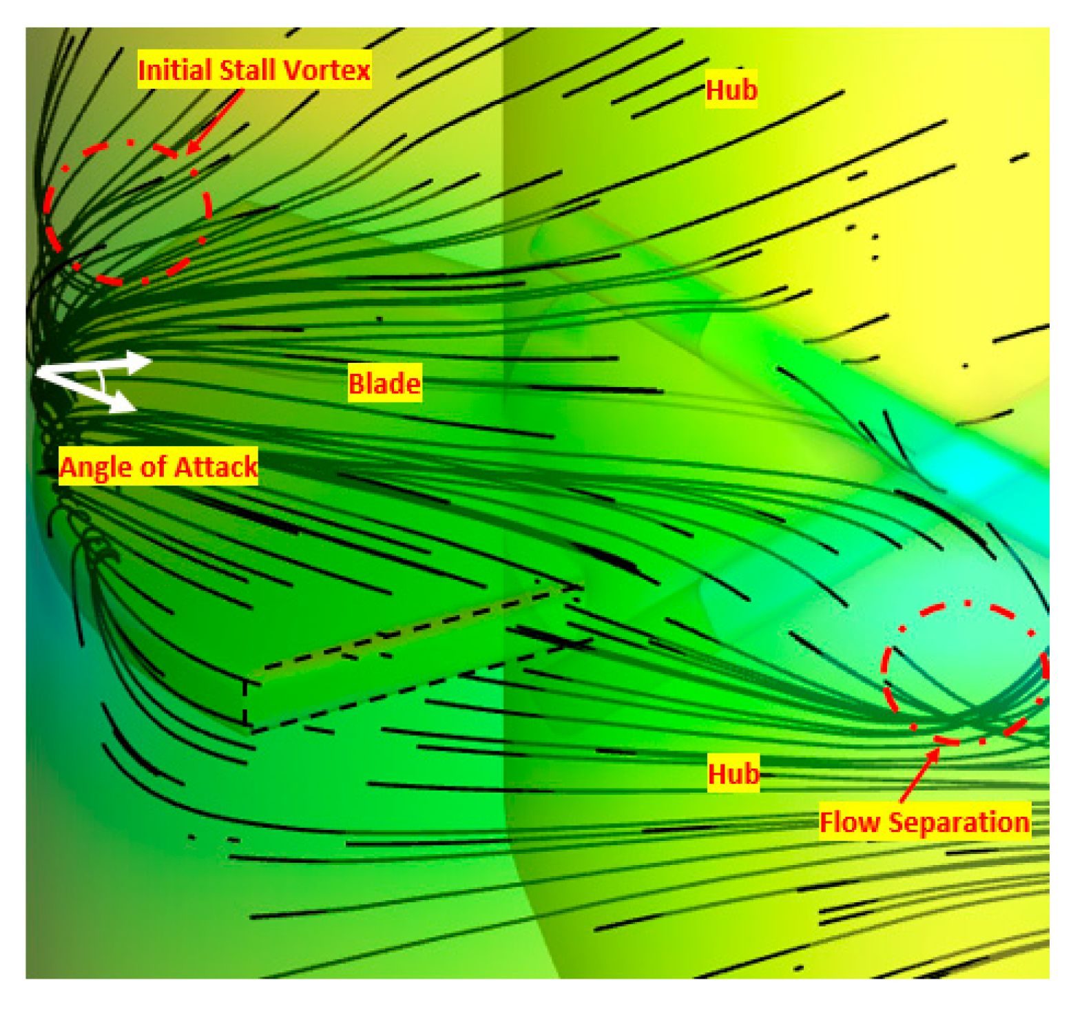
Figure 15 shows a three-dimensional streamline in an impeller flow tunnel under the 0.5 Qd condition. The impeller output is engulfed in a huge vortex, as seen in this figure. Near the impeller’s exit, over half of the flow passageways are blocked by vortex forms. The impeller loses more energy during blocking, because blocking causes more turbulence and turbulence dissipation. A larger angle of attack is created at the blade’s inlet as a result of the vortex spreading from the pressure side to the suction side of the blade and propagating to the next flow passage. The next flow passage splits as the impeller rotates, creating a stall vortex. As a result, the stall vortex moves in this instance in the opposite direction of the impeller spin.
5.7. Vortex Strength and Vorticity Distribution
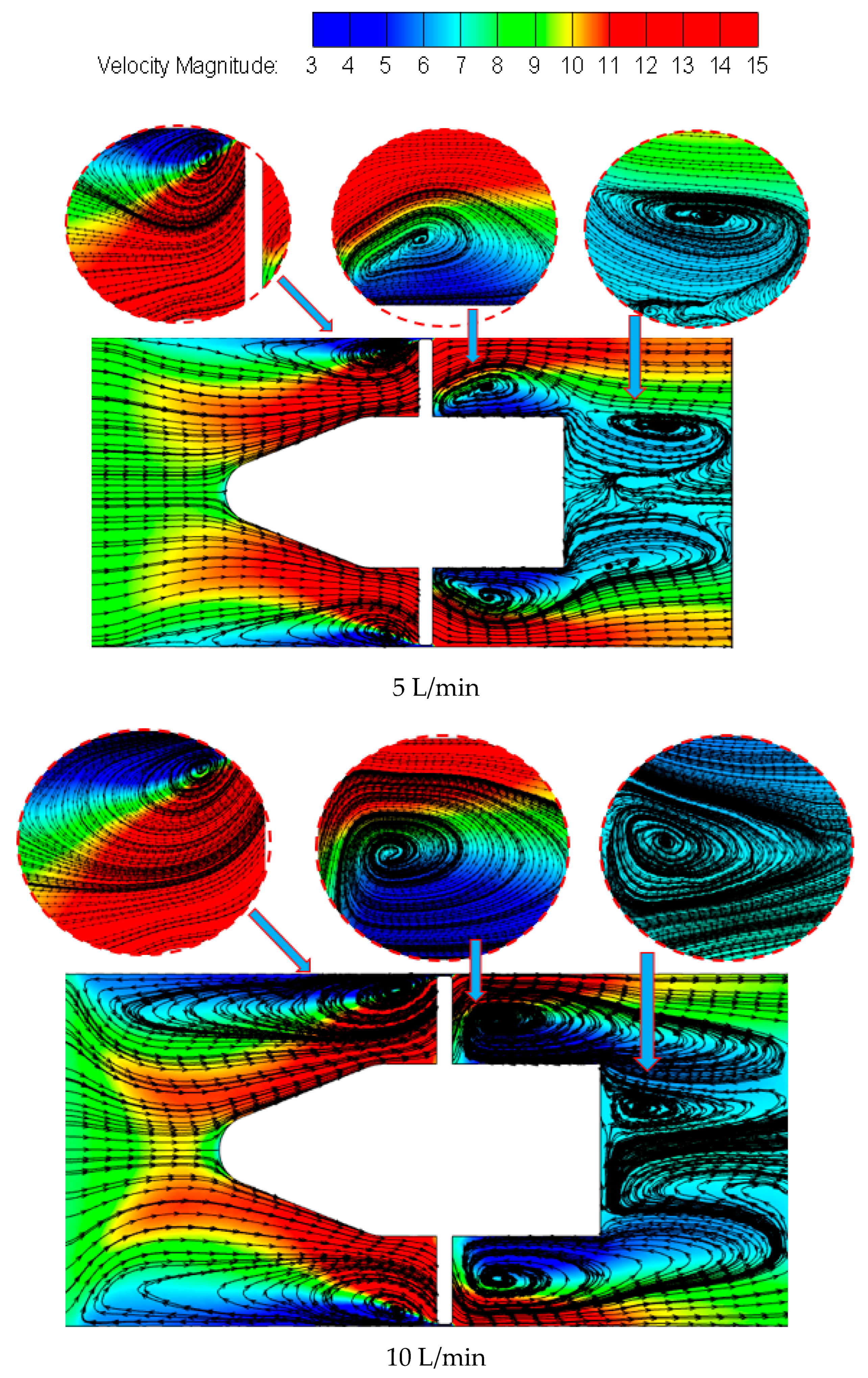
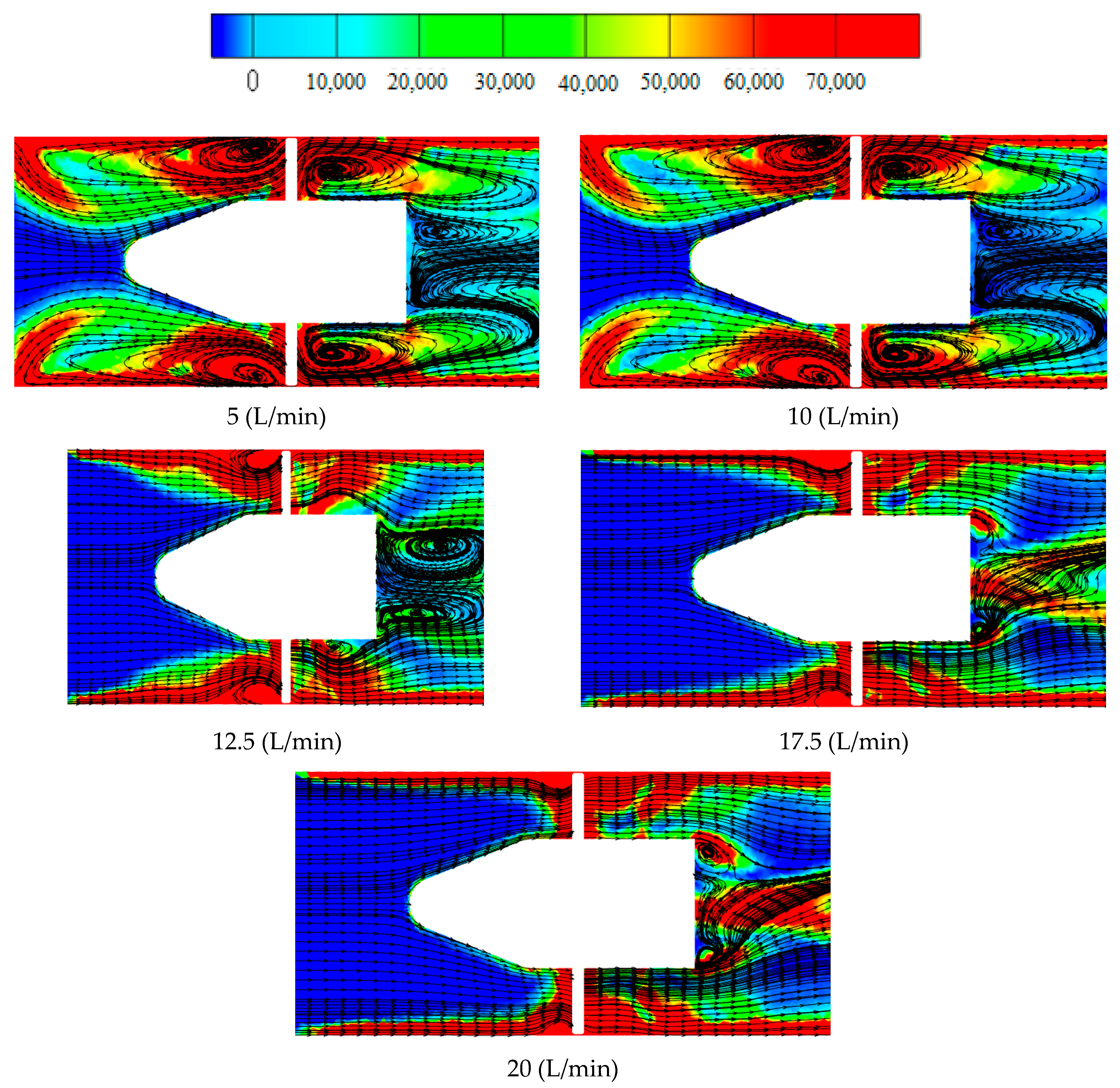
Figure 16 depicts the distribution of vorticity flow in each of the five flow conditions. The leakage shear zone and tip leakage vortex zone have a large amount of vorticity. There is a great deal of vorticity in the leakage zone and tip leakage vortex zones. Convection between the leakage flow and the main flow causes a vortex to form in the leakage shear zone. The vorticity in the tip leakage vortex zone adds to the vorticity carried by the leakage flow. In high-flow settings, vorticity has a significantly smaller effect than in low-flow situations. Induced vortices that developed in the end wall were contained within the tip leakage vortex zone.
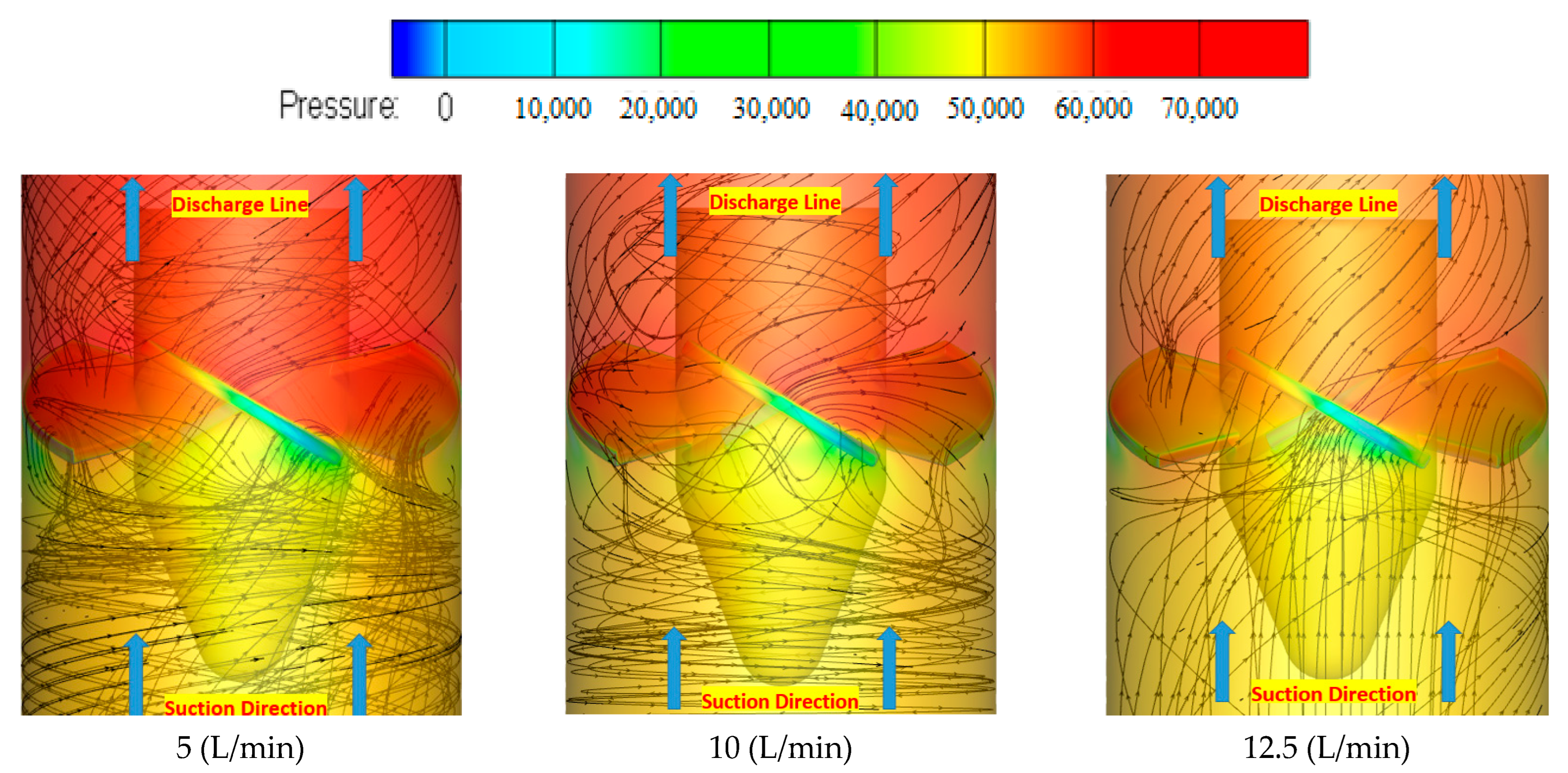
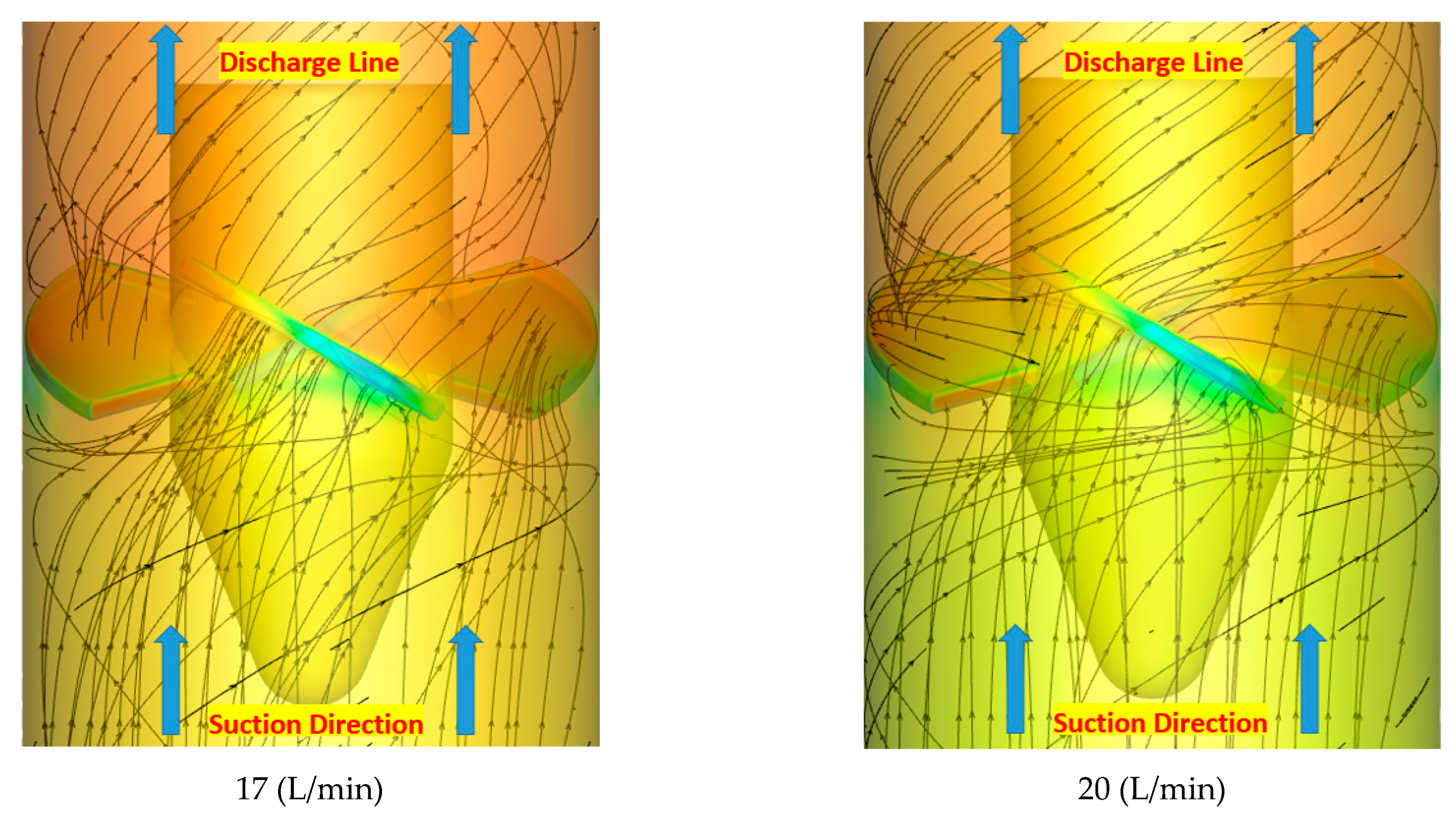
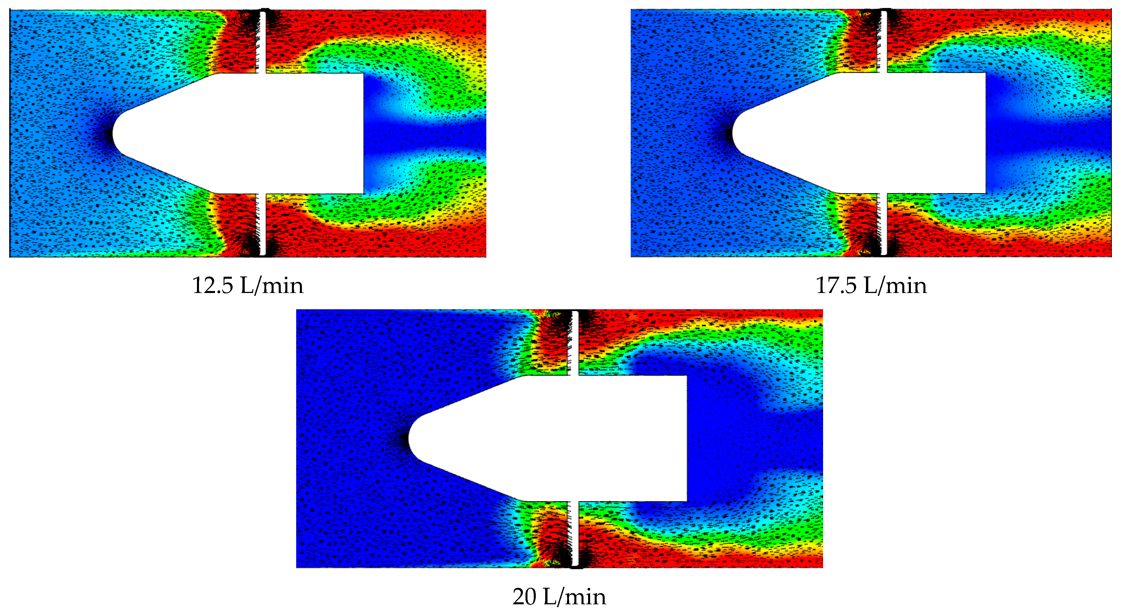
Figure 17 illustrates how the pressure of the pump varies under various circumstances. In this graph, the discharge line exhibits the highest pressure, whereas the blade tip exhibits the highest pressure. During low-flow circumstances, a sizable scale of secondary and vortex flows was also seen at the leading edge of the flow. The vortex radially and axially grew and shrank as a result. The vortex configuration changed from circular to spindle-like. It appeared to present low flow in the secondary case, but it was modest in high-flow conditions at the same position as the secondary flow and vortex. In the back of the blade, far from the suction surface, there existed a large vortex. As a result, the secondary flow and vortex seemed to have low flow, as previously mentioned, and their small size made it difficult for them to interact with the main flow.
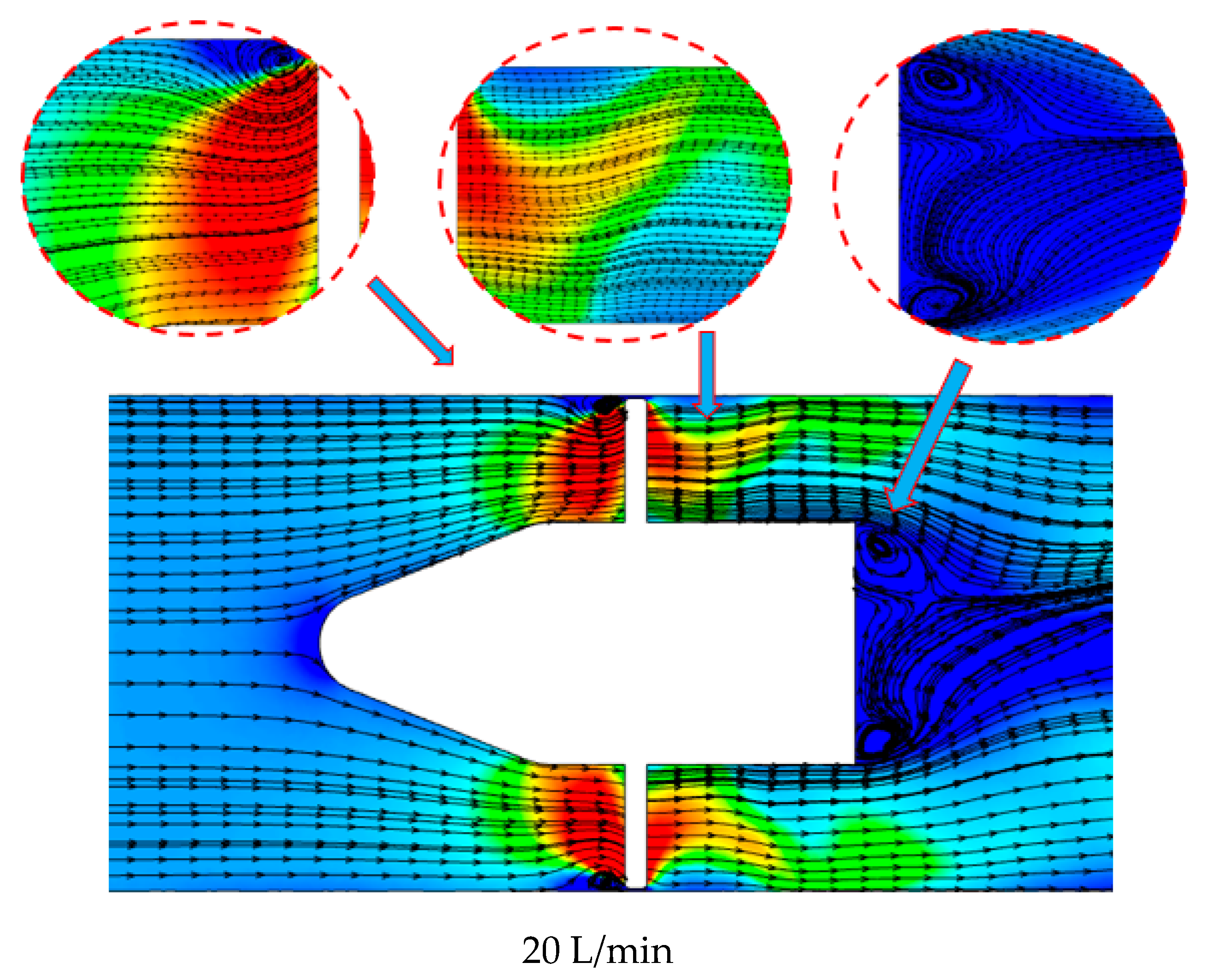
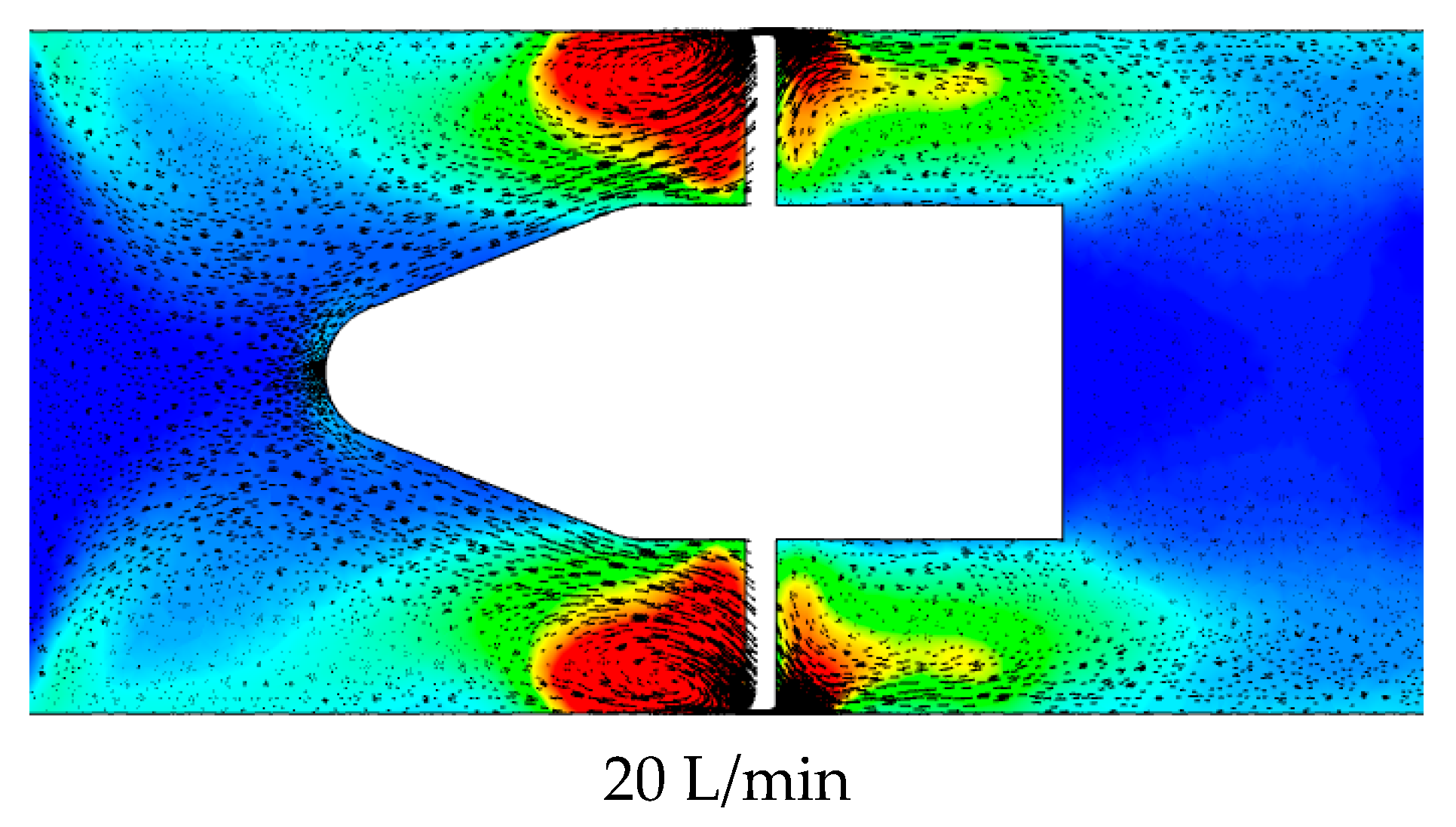
The circumferential velocity distribution of a vortex (
Figure 18) exhibits the transmission capability of the vortex. When the speed is modest, vortices have a tendency to gather in one location and radiate. In the various zones, which are depicted in this figure, secondary and vortex flows from mixed vapor and liquids were seen during low-flow circumstances. It is challenging for a leaky flow to generate an equally varied velocity due to the fluids’ mutual sharing. The secondary vortex is shifted, and the primary vortex is split from the subvortex. The vortex and secondary flow form diminish as the flow conditions increase.
Figure 10 depicts an independent leakage vortex flow under low-flow circumstances caused by the impeller rotation and flow superimposing on one another to form the leakage vortex flow.
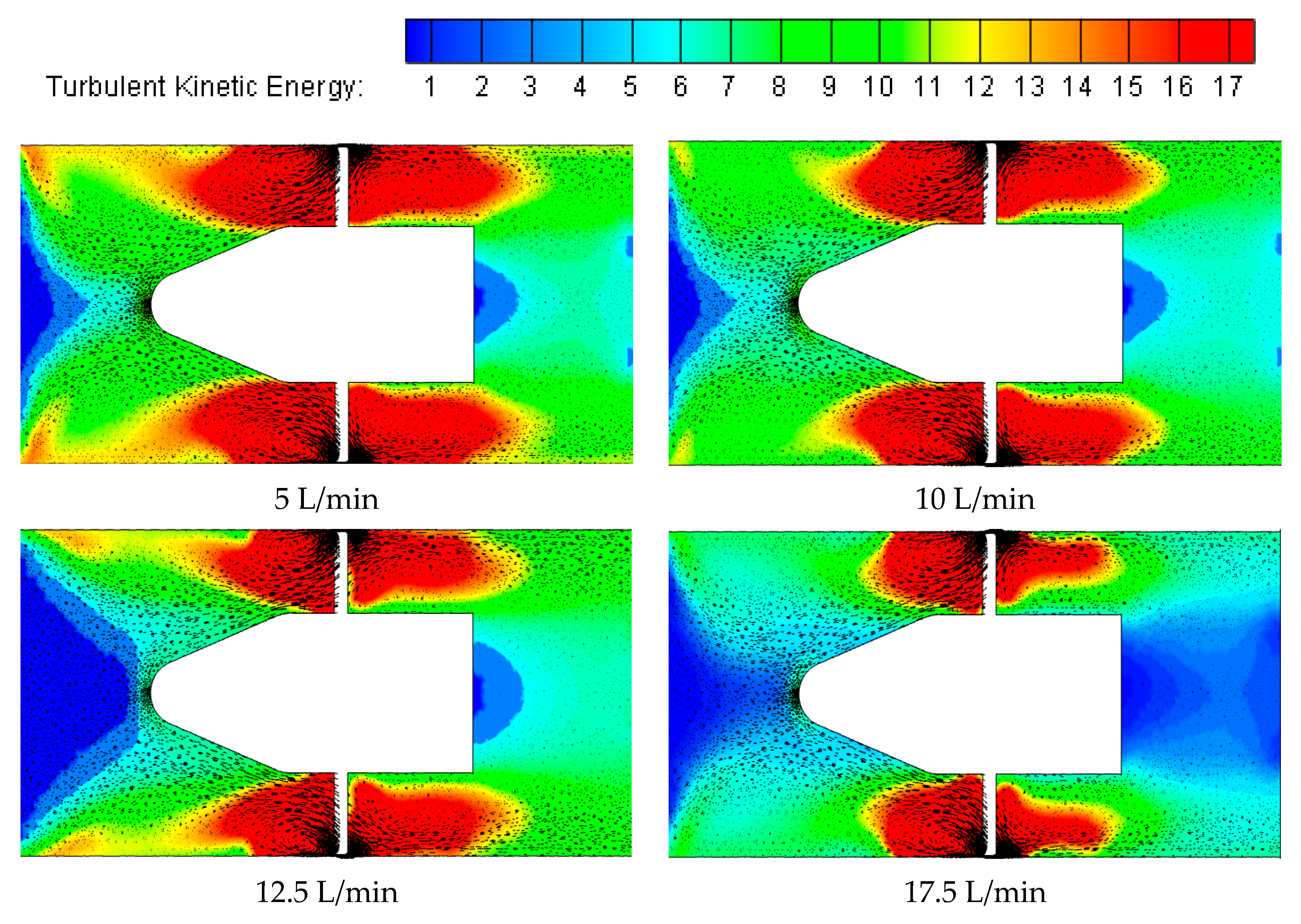
It was established that mixing flow and tip leakage vortices could be produced by the main flow as well as the mutual shear between the leakage flow and secondary flow. During the procedure, turbulent kinetic energy (TKE) was produced. The clusters of tip leakage vortices in
Figure 19 occupied the space that had previously been occupied by the initial leakage flow and the main flow convection, preventing the generation of turbulent kinetic energy where a secondary flow and mixing flow had evolved.
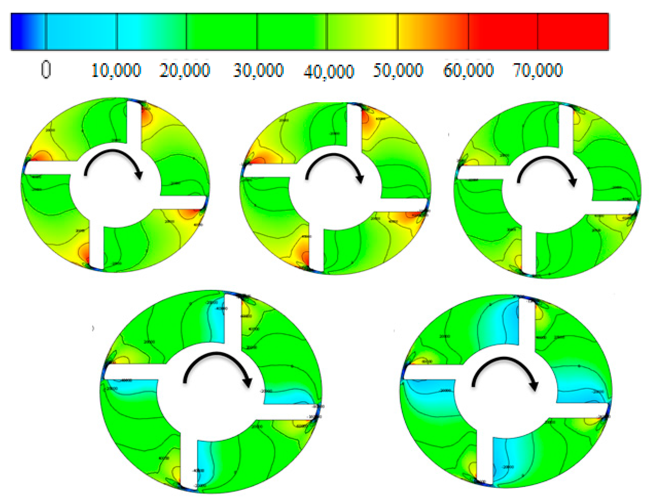
The analysis of the impeller with the internal flow field removed, as illustrated in
Figure 20, can be used to calculate the difference in pressure across the impeller axial flow pump’s pressure side. Axial flow pump flow patterns vary significantly depending on the flow circumstances. The flow patterns of the axial flow pump in this study changed. The axial flow pump showed a bias flow and vortex phenomena at the impeller inlet. The flow pattern was disturbed by a low-pressure region that formed close to the impeller rim as a result of clearance backflow. The hydraulic properties of a pump impeller are influenced by a number of parameters, such as clearance backflow. The problem of clearance backflow steadily diminishes as the pump flow rises. Axial flow pumps with impellers have refluxed clearances at the inlet and exit. Pump impellers exhibit action in their immediate surroundings quite clearly. As a result, when the pump flow increases, the effects of the clearance backflow on the pump impellers diminish. Full-tube pumps have an impeller with remarkable performance under conditions of high flow thanks to the design of the impeller.
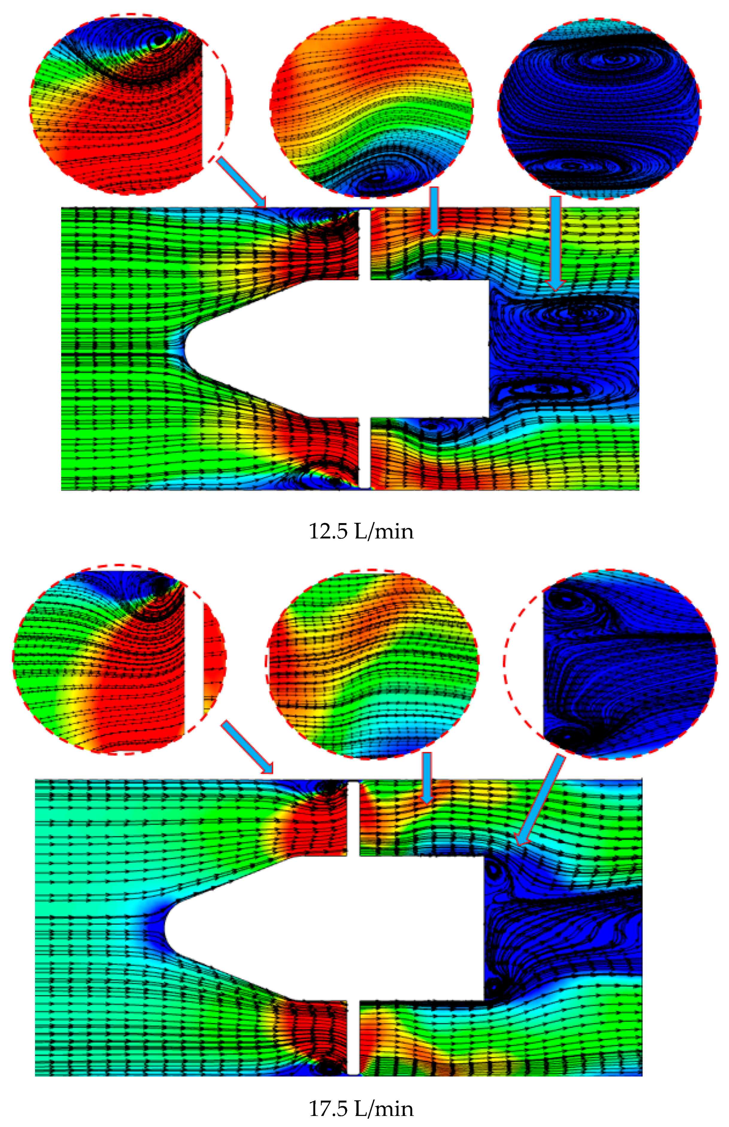
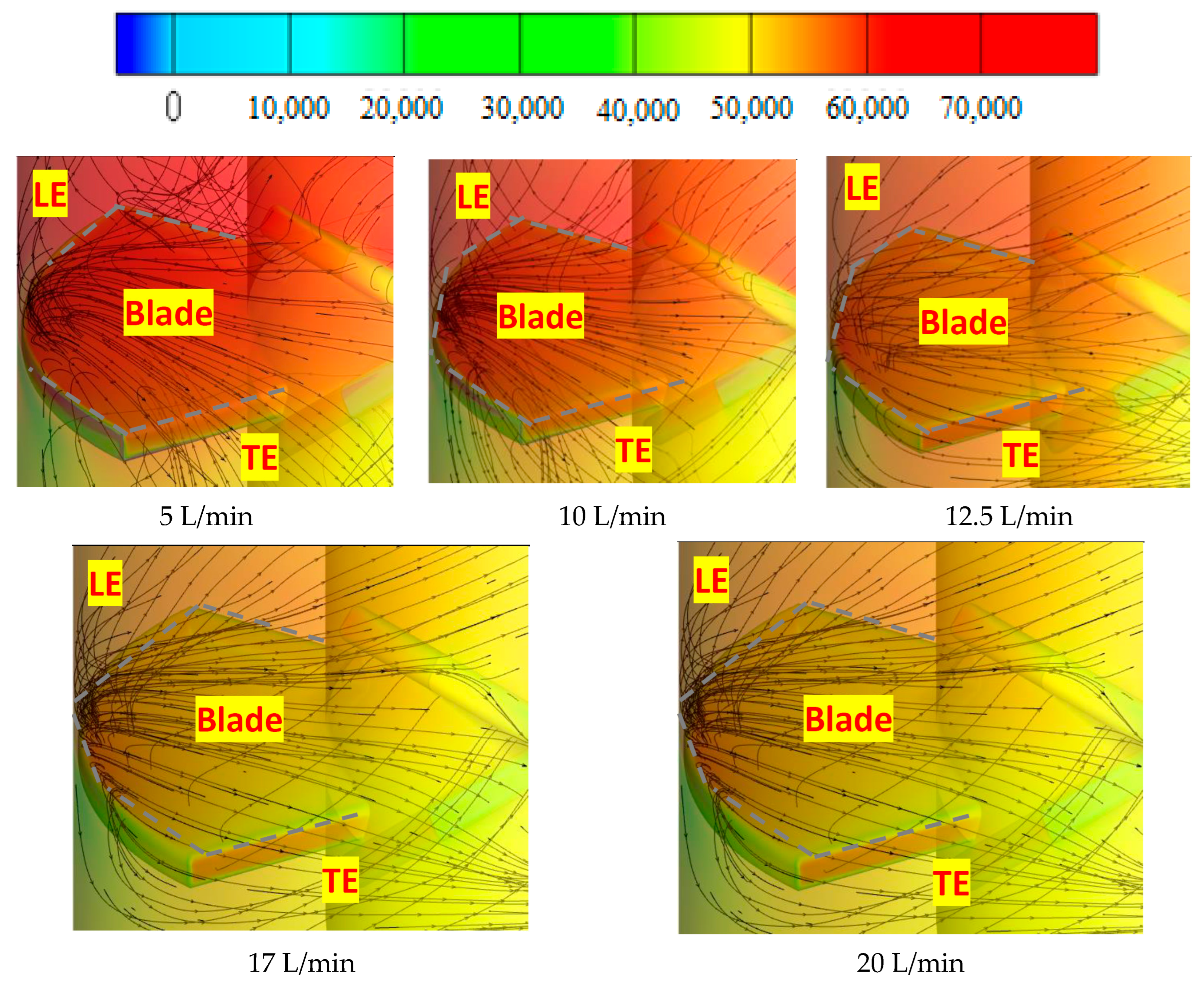
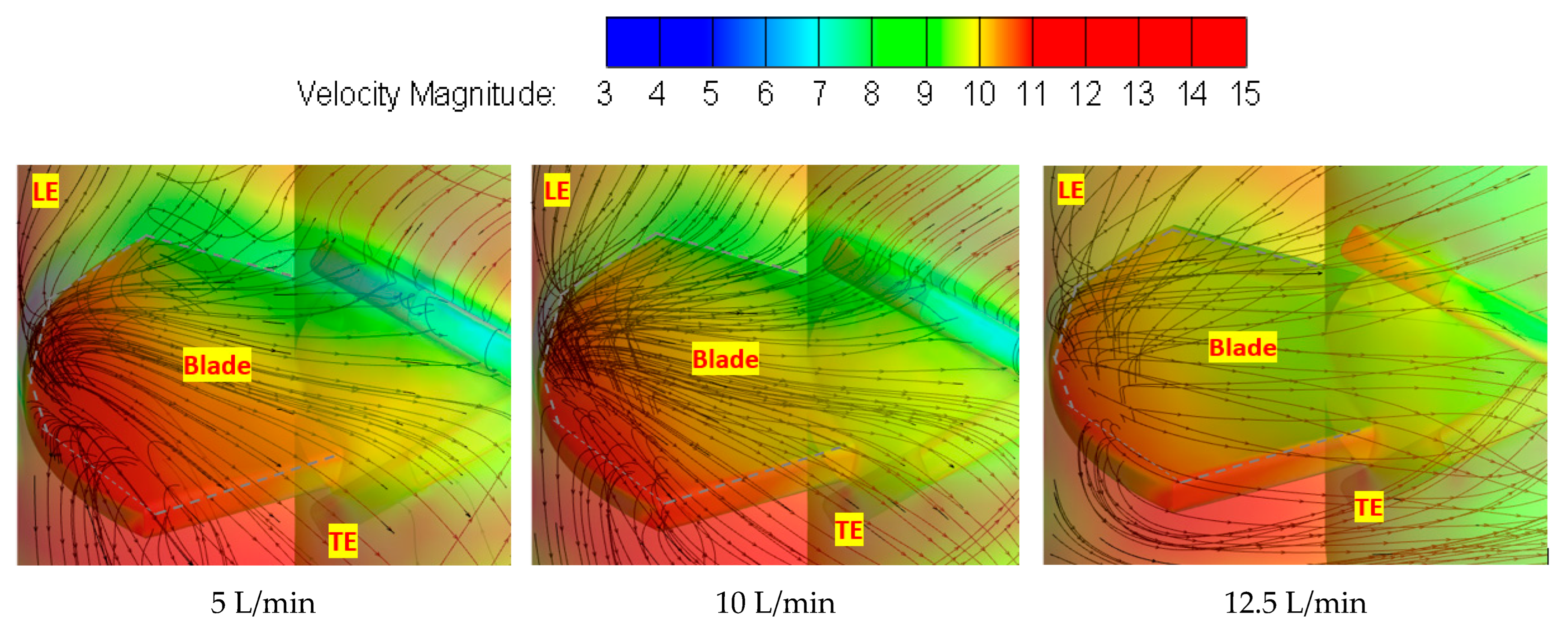
The motion vectors and static pressure contours on the blade surface change depending on the circumstances, as seen in
Figure 21 and
Figure 22. Under its design settings, the impeller’s flow field performs better than under other circumstances. The main flow near the entrance of the blade exhibits an increase in velocity in the axial plane and even has a tendency to shift in the opposite direction from the main flow as a result of tip leakage flow from nearby blades.
Tip leakage flow has a substantial impact on the main flow and exacerbates flow separation by creating greater counterclockwise vortices close to the suction side. As there is visible backflow, the suction pressure on the suction side steadily rises. Reduced flow rates cause an increase in pressure fluctuation, a drop in inlet flow angles, and an increase in incidence angle. At this point, the nearby vortex’s leakage flow causes the axial plane velocity to drop, increasing the circumferential velocity at the impeller’s inlet tip. Additionally, better flow separation leads to the greater separation vortex. The backflow is a result of the additional decrease in static pressure at the inlet edge brought about by the worsening of the pressure gradient. The static pressure steadily rises as the flow approaches the impeller inlet, and the separation becomes smaller.
5.8. Characteristics of Pressure Pulsations
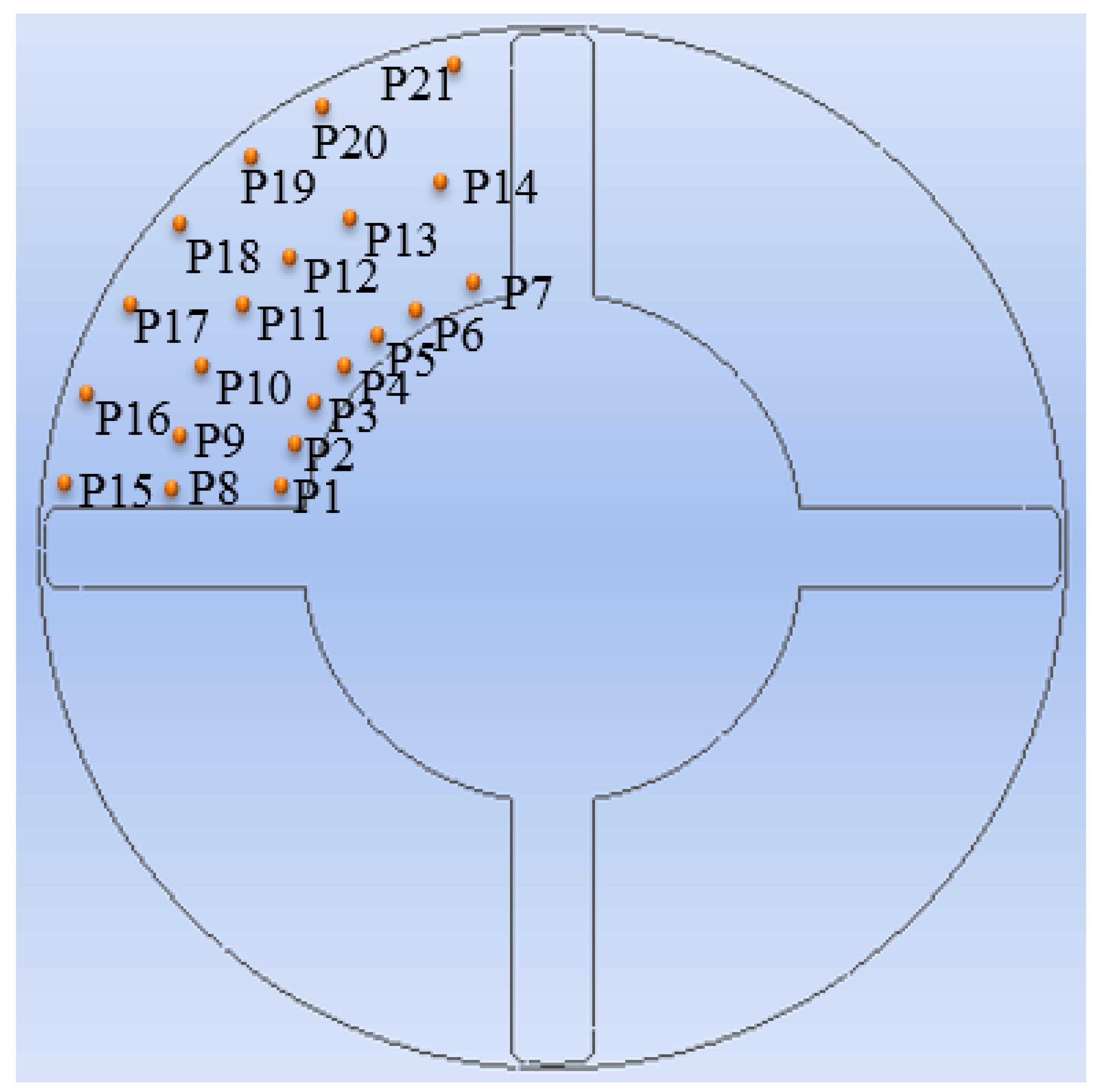
The performance of the axial flow pump’s pressure pulsation is examined by measuring the effects of the flow conditions at a total of 16 sites uniformly spaced from the blade impeller. According to
Figure 23, monitoring points P1 through P7 are situated close to the hub of the blade impeller, P8 through P14 are situated in the centre of the blade impeller, and P15 through P21 are situated at the outlet blade. The rotating frequency and pressure pulsation together determine a pump’s internal pressure pulsation characteristics.
The points shown in
Figure 16 were the locations of the observation spots. Impeller rotation was controlled by the monitoring locations.
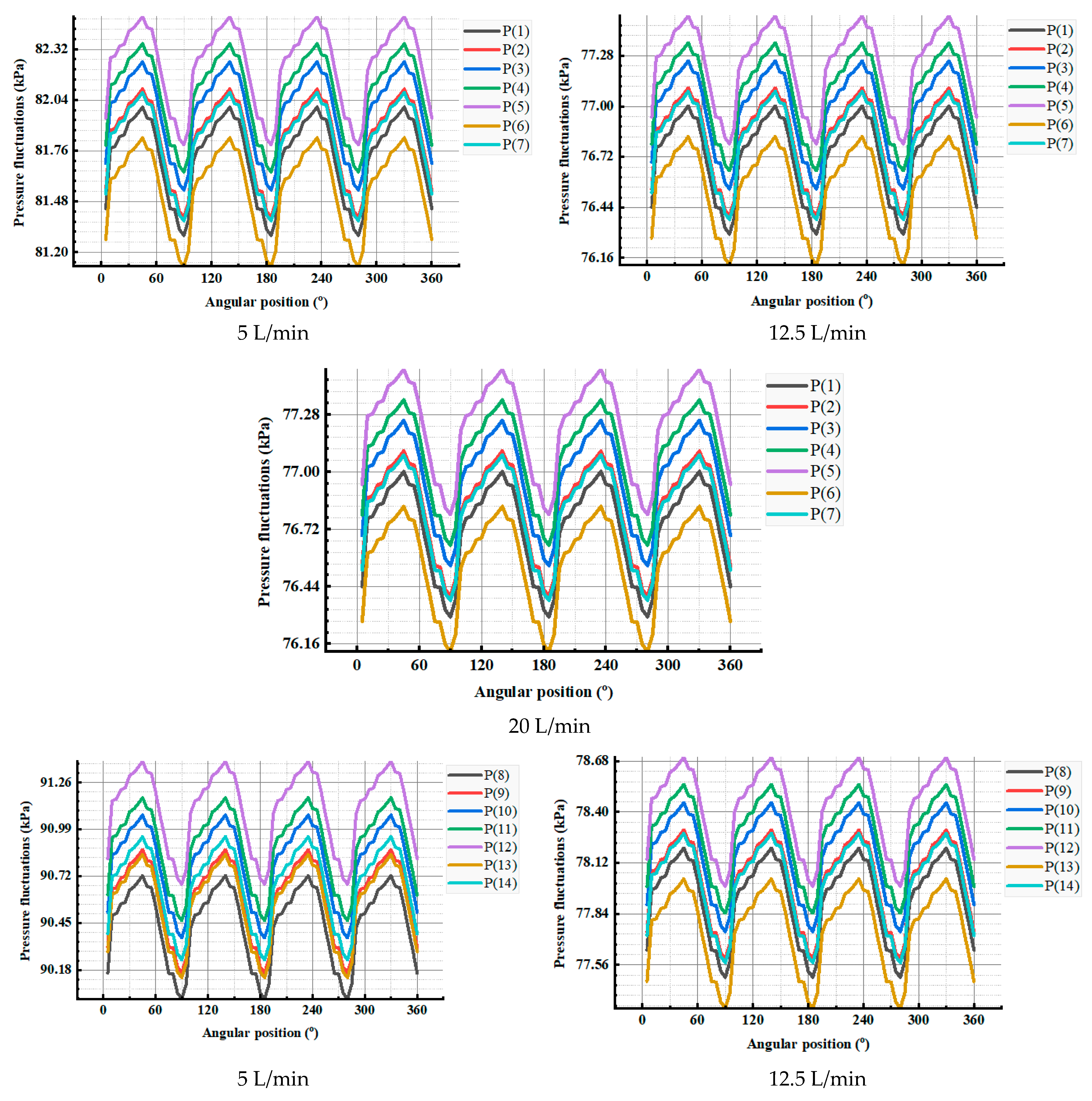
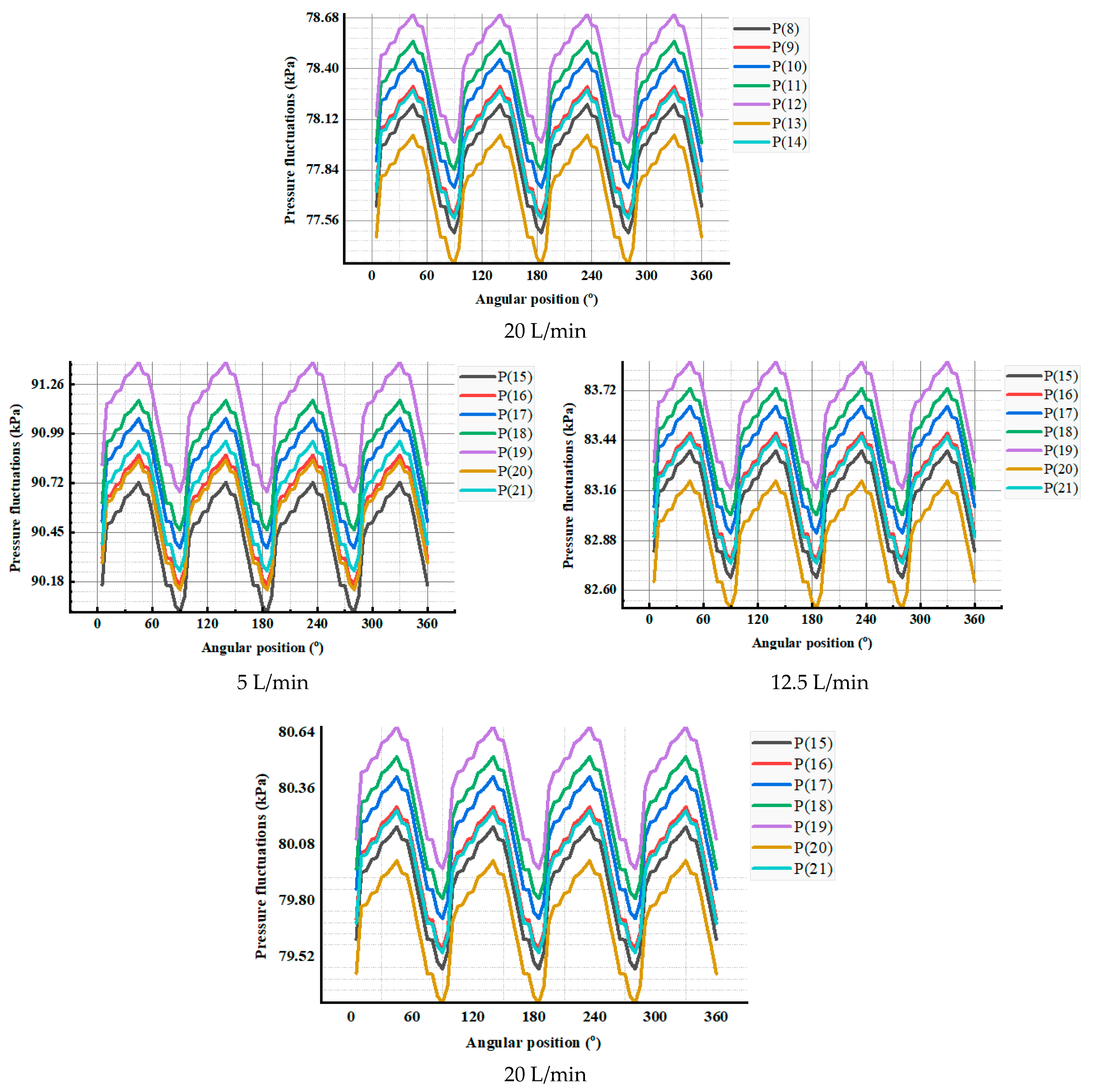
To evaluate and analyse the impacts of the flow conditions on the internal flow and pressure pulsations, the blade impeller sections were monitored under three working conditions (5, 12.5 design flow, and 20 L/min). The pressure pulsation can be observed in the time domain, as shown in
Figure 24. The pulsation curves for the monitoring points are also shown in
Figure 24. The figure demonstrates how the pressure pulsations changed depending on the flow operation conditions. The pressure pulsations’ amplitude increased together with the leading edge until the following edge reached its maximum size. Due to the secondary flow and vortex, the pressure pulsation amplitude was higher near the blade’s tip. The primary vortices were still entrained with one another. The pressure pulsation at the periphery of the vortex was enhanced by the high pressure close to the vortices as a result of the secondary flow distribution, and the pressure pulse amplitude was nearly equal to that at the core. The figures show four crests and four troughs after one impeller turn. In the temporal domain, axial flow pumps exhibit pressure pulsations that are comparable to those of axial flow pumps but have a different magnitude. In low-flow conditions, the pressure amplitude rose closer to the impeller. For the axial flow impeller, it was observed that when the flow rate increased, the pressure amplitude was reduced. When the flow rate was 5 L/min, the maximum pressure was recorded. The axial flow pump runs at the original design settings when the pressure pulsation amplitude is the most steady, according to the aforementioned data. Similar to this, the axial flow pump’s slow increase in pressure from hub to rim is seen in the image. Additionally, under some circumstances, the pressure pulsation’s amplitude at the impeller rose with the impeller radius, and the amplitude at the shroud’s P5 was almost 1.2 times that at the hub’s P8. The amplitude was roughly 1.21 times larger in the impeller’s P5 shroud than the hub’s P8 shroud.
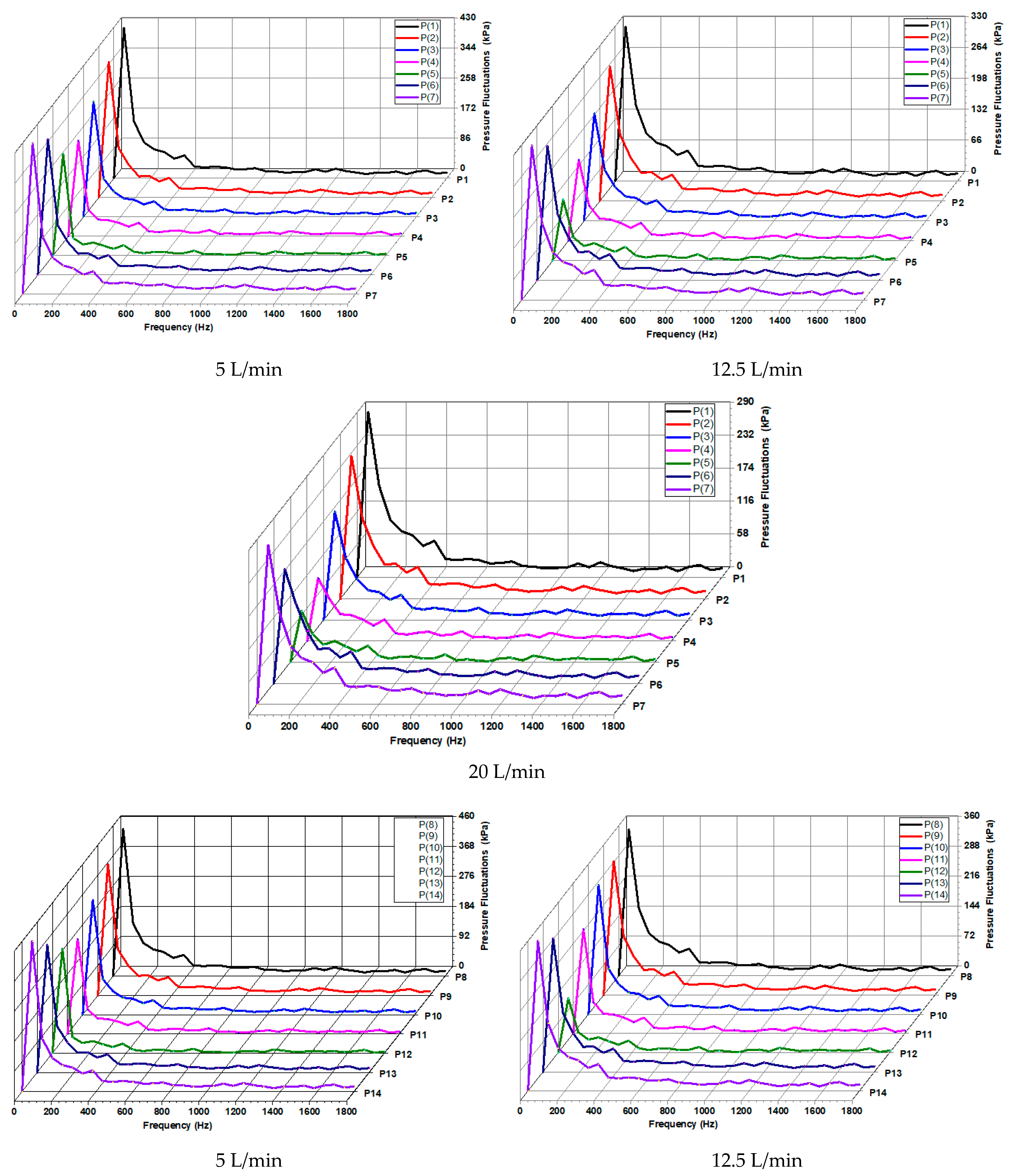
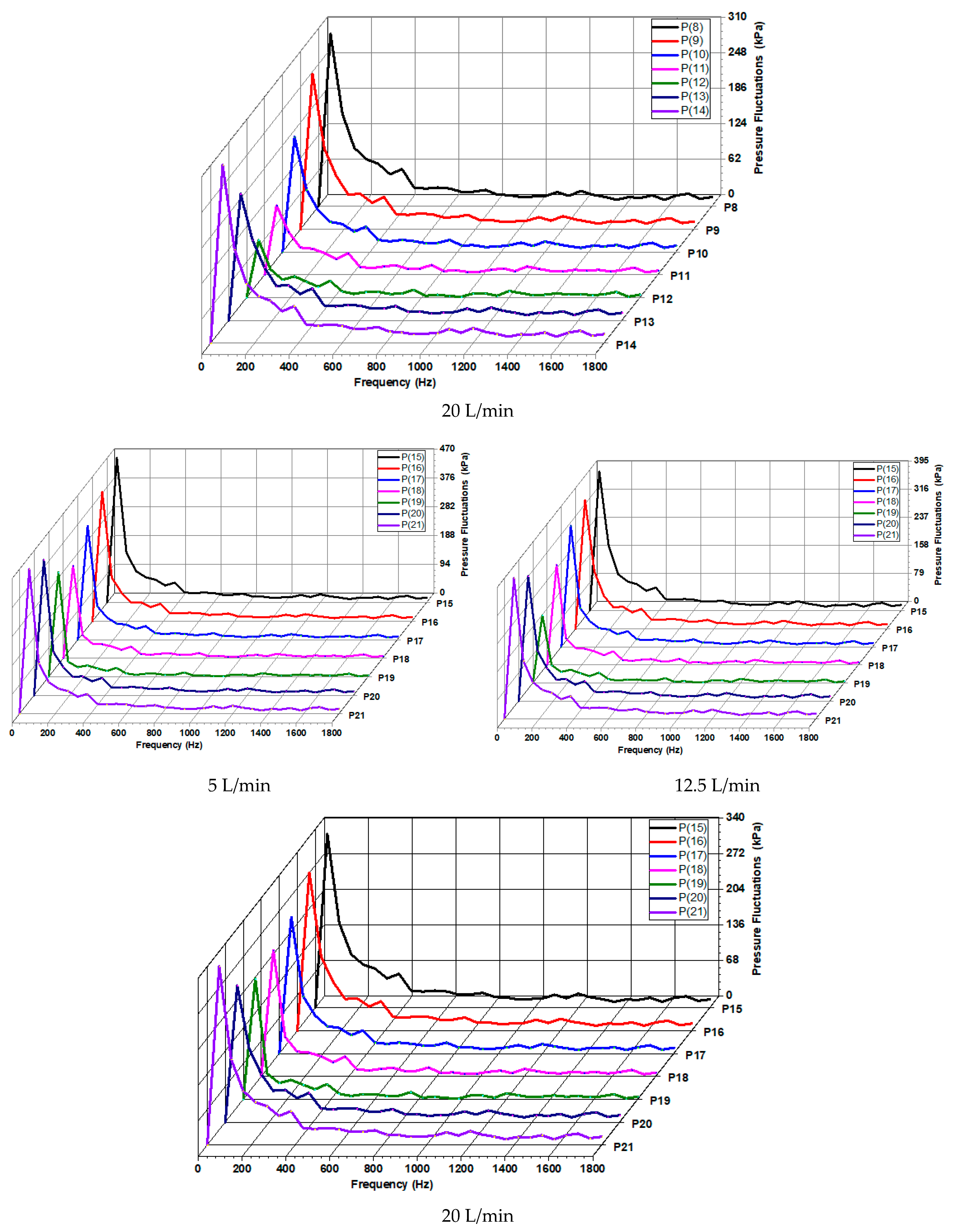
The pressure pulses under various operational situations were analysed in the frequency domain. CFD models were used to study the axial pressure fluctuations. The impeller blade was equipped with 24 monitoring points to show the flow characteristics of the pump under varied flow circumstances. First, a rapid Fourier transform was applied to analyse the pressure changes at three common flow rates. Under various circumstances, the pump’s pressure pulsation was measured.
Figure 25 depicts the findings. Three different flow rates associated with pump pressure fluctuations were examined using a fast Fourier transform. Various pump parameters were used to produce the pressure pulsation results. The flow field at the impeller’s input was impacted by the pump’s clearance backflow, which was significant under low-flow settings. Due to the vortices and deflections that were seen in the impeller inlet, it was found that low-flow circumstances caused an increase in the amplitude of the pressure pulsation. The clearance backflow capacity of the pump and the impact on the inlet flow field varied under high-flow conditions.
The primary frequency amplitude was significantly different at all monitoring points of the axial flow impeller tip blade than it was at all other locations. An amplitude difference of 1.12 and 1.01 times was seen between the two components of the axial flow pump between monitoring points P1 and P5, respectively. At monitoring point P5, in comparison to reading point P8, an amplitude of 1.07 times was recorded. Between P1 and P5, the amplitude differences were around 0.73 and 0.62 times greater than those between the areas of the axial flow pump. Under the conditions of P5 and P8, as opposed to P1 and P4, the overall amplitude of the pressure pulsations in the event of limited flow is larger. As a result, the rotation of the impeller causes the pressure pulsations in the input portion.
The amplitude of the primary frequency at all monitoring locations for the axial flow pump tip blade differed significantly from all other portions of the impeller. At monitoring points P1 and P5, an amplitude difference of roughly 1.12 and 1.01 times was seen for both components of the axial flow pump. P8 had a reading that was 1.07 times greater than P5, which was monitored by the amplitude. The amplitudes in the axially pumped regions P1 and P5 were greater by 0.73 and 0.62 times, respectively.
6. Conclusions
Axial flow pumps were examined using CFD and model testing to establish their hydraulic performance and pressure pulsation characteristics. Moreover, in the present study, the pressure pulsation properties of axial pumps were investigated. A numerical simulation of an axial flow pump was performed in unstable settings. The quantity of clearance reflux changed the pump’s pulsation pattern as a result of the pressure pulsation. The results provide information about how pumps operate. The study also examined the impeller’s internal flow behaviour and the pressure pulsation characteristics, leading to several conclusions. The findings of the study demonstrate that the flow circumstances have a considerable impact on the leaking vortex form and flow characteristics, including the chordwise distribution of the pressure differential. Transverse sections revealed that the distribution of the vortex strength varied with the flow conditions, increasing the vortex distribution. As a result, the average vortex distribution dispersion rose. A multitude of factors, including secondary flows, mixing flows, and vortices, contributed to the pressure pulsations. Their spread varied in speed. The kinetic energy of turbulent flows changed as a result of the inhibition of the shear between the leaky flow and main flow. The inlet pressure of an axial flow pump exhibits pressure pulsations as a result of the impeller’s rotation. The magnitude of the pressure pulsation rises with increasing distance from the impeller. The frequency at which the blades pass one another is the main contributor to pulsing pressure. Under the same circumstances, the impeller’s inflow amplitude gradually increases with the pump radius. At the same monitoring site, the main frequency of the pressure pulsation’s amplitude gradually decreases with the flow rate. It is clear from the numerical simulations and model tests that the impeller pump creates a larger pressure amplitude when there is little or no flow. With little flow, there is significant clearance backflow due to the pump’s huge clearance.
In the future, we will study the effect of cavitation flow conditions in axial pumps based on different methods, such as vibration, acoustics, current, and CFD.


