Numerical Simulation Study of Pressure-Driven Water Injection and Optimization Development Schemes for Low-Permeability Reservoirs in the G Block of Daqing Oilfield

Abstract

Pressure-driven water injection technology shows significant potential in addressing the key challenges of low-permeability oil reservoirs, improving water flooding development efficiency. Grounded in FDEM theory, this study establishes fluid matrix constitutive equations and employs FDEM to resolve rock stress–strain fields. A numerical simulation method for pressure-driven water injection in low-permeability reservoirs is developed to study the impact of different well pattern densities. The results indicate that the 90° horizontal well pattern using the five-spot method yields optimal outcomes, with approximately 32.32% higher cumulative liquid production than vertical well patterns. The 45° horizontal well pattern with the reversed nine-spot method also performs well, with about 30% higher cumulative liquid production than single-row vertical wells. Pressure-driven water injection improves matrix oil–water permeability and expands water flooding coverage. Based on the pressure gradient distribution driven by different well patterns, an evaluation method for the inter-well utilization capacity and its effectiveness was established. This method quantitatively assesses the reservoir depletion under various horizontal well encryption schemes. For research on timing of water injection in pressure-driven water flooding. Compared to pressure-driven water injection after 90 days, there is increased cumulative oil production after 40 days, emphasizing the importance of early pressure maintenance for higher cumulative oil production and enhanced recovery rates in low-permeability reservoir development. These findings provide crucial theoretical and practical support.

1. Introduction

China boasts vast reserves of low-permeability reservoirs, presenting substantial development opportunities. The efficient and economically effective exploitation of these low-permeability reservoirs is crucial for achieving consistently high-level oil and gas production in China. Water flooding, a fundamental technique in the development of low-permeability reservoirs, offers notable benefits, including substantial incremental recovery and the rapid enhancement of reservoir energy [1,2]. Nevertheless, the practical application of water flooding technology encounters notable variations in effectiveness due to the distinctive characteristics of individual reservoirs. In areas characterized by localized fractures, water injection frequently faces challenges, notably preferential flow along these fractures, which can lead to water channeling and ineffective injection. Consequently, addressing the challenge of unlocking the untapped potential of low-permeability reservoirs calls for customized water injection strategies that take into account the distinct characteristics of each reservoir. This approach is designed to fine-tune water injection plans and capitalize on reservoir potential through precise water injection, acknowledging the variations among different reservoirs. A pertinent example of site-specific technologies is G Block in Daqing Oilfield.

The development of the G Block in Daqing Oilfield has progressed into its intermediate and advanced stages. Extensive water injection has left a considerable volume of untapped oil reserves and a lower-than-desired recovery rate. Researchers have been diligently exploring the optimal wellbore configuration and network design that can effectively boost water flooding recovery rates [3,4,5]. In the context of the study on the five-spot method, Xiao et al. [6] proposed that the five-spot well pattern exhibits significant potential for enhancing methane recovery in coal bed methane reservoirs. Wang et al. [7] conducted a comprehensive study on the repeated fracturing mechanisms of vertical and horizontal wells within low-permeability tight oil reservoirs, specifically employing the five-spot well pattern. They elucidated the effects of repeated fracturing in low-permeability reservoirs within the framework of the five-spot well pattern. Wang et al. [8] introduced an innovative method for calculating the production capacity of high-order water-bearing stages in a five-spot well pattern. Their findings demonstrated that, as fracture length and pressure difference increase, production capacity also rises significantly. Additionally, Xie et al. [9] delved into the influence of permeability anisotropy on the development effectiveness of the five-spot well pattern. They contributed a general analytical solution for the layout of the five-spot well pattern, which serves as valuable theoretical guidance for the rational construction of this pattern in anisotropic reservoirs. Yu [10] conducted research on the water injection methods in a closely spaced well network within Daqing Oilfield and concluded that the five-spot pattern excels in achieving precise control over water flooding. Furthermore, Liu [11] advocated the application of the five-spot well pattern as the optimal development approach for low-permeability sandstone and gravel reservoirs. This pattern significantly enhances recoverable reserves, particularly during the high water-cut phase of reservoir production. Du et al. [12] explored well spacing for polymer injection in a five-spot well pattern and the results indicated that the most efficient range for well spacing falls between 150 and 180 m. Bu [13] proposed a theoretical explanation for the average reservoir pressure in the context of the five-spot well pattern. This theory not only forms the basis for the efficient development of reservoir blocks but also provides valuable insights applicable to the development of other oilfields. The study has comprehensively addressed production issues related to the five-spot well pattern. However, there is currently limited research on encryption schemes specifically tailored for the five-spot well pattern. Therefore, this study focuses on investigating production aspects concerning the encryption scheme for the five-spot well pattern.

The nine-spot wellbore configuration is a widely adopted pattern in oilfields, and numerous scholars have conducted extensive research in this area. Zhang et al. [14] utilized a flow tube model to solve the saturation distribution field of the inverted nine-spot well pattern. They introduced an innovative approach to study the theoretical water cut growth rate in water-flooded reservoirs. Xia [15] explored the impact of layer-damaged wells on production. By comparing three methods—namely, the inverted nine-spot well pattern, the seven-spot well pattern, and the five-spot well pattern—they provided a theoretical basis for the comprehensive management of layer-damaged wells. Considering the specific characteristics of low-permeability reservoir water injection development, Ji et al. [16] introduced a production calculation formula tailored for the inverted nine-spot well pattern. Lian [17] presented an analysis that took into account the fracture conditions in the inverted nine-spot well pattern’s injection–production relationship. A model for calculating water breakthrough time is established which considers factors such as injection–production pressure differential anisotropy; this provides effective theoretical support for the development of low-permeability fractured reservoirs. Li et al. [18] investigated a production calculation model for variable initiation pressure gradient area well patterns based on pressure sensitivity effects. They proposed a model specifically for the inverted nine-spot well pattern, which can be utilized to assess reservoir depletion under various well pattern conditions. Zhang [19] conducted research on the dynamic changes in oil–water wells using the slanted inverted nine-spot well pattern, analyzing production change patterns and the main factors affecting the decline in liquid production. Zhu et al. [20] conducted research on production calculation for diamond-shaped inverted nine-spot well patterns in low-permeability reservoirs. Scholars have made significant research contributions in terms of saturation distribution, production calculation, and reservoir evaluation in the context of the inverted nine-point method. However, there is currently a lack of systematic academic research on the encryption scheme issues associated with the reverse nine-point method. This area of study is relatively underexplored, with limited in-depth exploration and thorough analysis. Therefore, academic discussions and theoretical expansions in this field remain relatively unexplored, necessitating further attention and in-depth investigation from scholars. Research in this area not only aids in filling knowledge gaps but also provides valuable references and guidance for optimizing the application of the inverted nine-point method.

After the G experimental area commenced production in 2016, adjustments were made to the injection–production system with the goal of establishing a linear water flooding development approach. However, this approach has brought forth several issues. These include a continuous decline in the water intake capacity of injection wells, a rapid decrease in oil well production, and severe backpressure in oil–water wells. These problems signify the absence of an effective reservoir drive system. To tackle these challenges, a volume fracturing approach has been introduced, which involves the densification of horizontal wells and pre-fracturing. This process aims to restore reservoir pressure to 100–120% of its original level. As a result, the flow field transforms into unstable seepage with varying liquid flow directions. This transformation significantly enhances the reservoir’s seepage capacity and further increases the production capability of the experimental area. It is important to note that the G experimental area contains small-scale sand bodies with poor physical properties. Presently, water flooding control within the well network is inadequate, resulting in poor water flooding development effectiveness. Additionally, an effective drive system has not been established between wells, leading to low reservoir utilization. Research findings suggest the presence of remaining oil reserves in the experimental area. To address these issues, horizontal well densification is being implemented in the main oil-bearing strata. Utilizing the conditions of the well group’s fracture network, efforts are being made to improve oil recovery. In the later stages of development, various supplementary reservoir energy approaches are being explored to significantly enhance the degree of oil recovery in the block. In this study, based on the low-permeability reservoir in the G block, a numerical simulation method for water flooding has been established. It focuses on studying the impact of different water injection well densification methods on development outcomes.

2. Block Geological Description

As depicted in Figure 1, the G experimental area is situated in the southwestern part of the Fenshentun Anticline’s northwest flank, which is located in the central depression of the northern Songliao Basin. Based on well–seismic integration and detailed structural interpretation, the overall structural configuration of the experimental area is characterized as a west–northwest dipping monocline controlled by north–south trending faults. The strata exhibit a relatively steep dip angle of approximately 5.5° with an average slope gradient of 96 m/km. Notably, the shallowest point of burial in the southeast reaches a depth (sea-level depth) of −1112 m, while the deepest point in the north is at a depth of −1274 m, resulting in a depth difference of 162 m. The region is marked by predominantly north–south-oriented faults, all of which are normal faults. These faults have lengths ranging from 2.0 to 3.5 km and fault throws varying from 20 to 60 m. Additionally, the dip angles of these faults range from 40 to 70 degrees. In terms of fault density, there are approximately three faults per square kilometer in this area.

Transitioning from the sedimentation of the Deng Louku Formation into a stable subsidence period, structural activity was low, with abundant lake water, and a plentiful supply of sediment. Sediments rapidly and steadily accumulated during this time. As we approach the end of the Nenjiang Formation, the strata began to experience compression and subsequent uplift, entering a phase of reverse uplift. The current structural pattern has taken shape, and the late-stage tectonic background has imparted excellent vertical continuity to the structural features.

3. Algorithm Principle

In order to improve the computational efficiency of the model for the waterflooding process in enhanced oil recovery, certain fundamental assumptions have been integrated into the waterflooding model: 1. Solid elements are impermeable. 2. Connection elements allow bidirectional fluid flow. 3. Joint elements use the initial aperture “a₀” to represent the permeability of the rock matrix. The finite difference element method (FDEM) is employed as a numerical simulation technique that astutely combines the strengths of both continuum and discontinuum methods. In FDEM, the computational domain is discretized into triangular finite element elements. Along the boundaries of these finite element elements, four-node cohesive elements with negligible thickness are introduced. As joint elements fracture, the initial aperture of these elements increases, subsequently raising the permeability of the rock matrix. Consequently, this approach effectively characterizes flow at both the pore and fracture scales.

3.1. Motion Control Equations

FDEM employs a second-order finite difference method to solve the motion equations for each time step. These equations are derived from the mass and forces acting on nodes, resulting in the computation of velocities and displacements of nodes, along with updates to their coordinates. The motion control equations are rooted in Newton’s second law and factor in the effects of viscous damping.

$$\mathrm{M}\frac{{\mathit{\partial }}^{2}X}{\mathit{\partial }{t}^2}+C\frac{\mathit{\partial }X}{\mathit{\partial }t}=F$$

(1)

where M represents the node mass matrix, C stands for the viscous damping matrix, t denotes the time step, X is the node displacement vector, and F is the node force vector. The node force vector encompasses various components, such as the elastic deformation force of triangular elements, the elastic–plastic deformation force of node elements, and the contact force between discrete elements. The primary purpose of the viscous damping matrix is to mitigate the influence of stress wave oscillations in the model. Its equation is as follows:

$$C=\mu I$$

(2)

$$\mu =2h\sqrt{\rho E}$$

(3)

where I is the identity matrix, μ is the viscous damping coefficient determined by the single-degree-of-freedom mass–spring system, h is the element length, ρ is the element density, and E is the element elastic modulus.

3.2. Element Damage Model

Modeling fractures in joint elements is a crucial part of FDEM. Under external forces, joint elements connecting adjacent triangular elements can close, open, or slide tangentially. The normal displacement of the joint element is denoted as O, and the tangential displacement is denoted as S. The damage variable D for the joint element can be defined as follows:

$$D=\left\{\begin{array}{ccc}0& O<O_p,S<S_p& undamaged\\ \frac{O-O_p}{O_r-O_p}& O\ge O_p,S<S_p& tensile failure\\ \frac{S-S_p}{S_r-S_p}& O<O_p,S\ge S_p& shear failure\\ \sqrt{{\left(\frac{O-O_p}{O_r-O_p}\right)}^2+{\left(\frac{S-S_p}{S_r-S_p}\right)}^2}& O\ge O_p,S\ge S_p& tensile-shear failure\end{array}\right.$$

(4)

where O_p represents the normal displacement when the normal stress on the joint element equals the pure tensile strength. S_p represents tangential displacement when the tangential stress on the joint element equals the pure shear strength. O_r and S_r represent the normal and tangential displacements, respectively, when the joint element undergoes pure tensile and pure shear failure, which are the critical failure displacements. The equations for calculating O_p, S_p, O_r, S_r are as follows:

$$O_p=\frac{2h{f}_t}{pf}$$

(5)

$${\mathrm{S}}_p=\frac{2h{f}_s}{pf}$$

(6)

$$O_r=O_p+\frac{3G{f}_{\mathrm{I}}}{f_t}$$

(7)

$${\mathrm{S}}_{\mathrm{r}}=S_p+\frac{3G{f}_{\mathrm{I}\mathrm{I}}}{f_s}$$

(8)

where h represents the length of the joint element. pf is the penalty parameter for the joint element. f_t is the tensile strength of the joint element. f_s is the shear strength of the joint element, which can be obtained using the Coulomb–Mohr equation:

$$f_s=-\mathrm{\sigma }\tan \left(\mathrm{\phi }\right)+c$$

(9)

If the calculated damage variable D based on Equation (4) is greater than 1, then it is assumed that D = 1, indicating that the joint element has fractured and will no longer participate in subsequent stress calculations for joint elements. Based on the damage variable D of the joint element, reduction factors for the tangential and normal stresses of the joint element, denoted as D, can be obtained.

$$f\left(D\right)\left(1-\frac{a+b-1}{a+b}{e}^{\left(\frac{D(a+cb)}{(a+b)(1-a-b)}\right)}\right)\left(a(1-D)+b{(1-D)}^c\right)$$

(10)

where a, b, and c are experimental parameters. The normal stress and tangential stress of the joint element can be expressed as follows:

$$\mathrm{\sigma }=\left\{\begin{array}{c}\frac{2O}{O_{\mathrm{p}}}{f}_t,O<0\\ \left(\left[\frac{2O}{O_{\mathrm{p}}}-{\left(\frac{O}{O_{\mathrm{p}}}\right)}^2\right]f_t\right)\\ f\left(D\right)f_t,O>O_p\end{array}\right.f\left(D\right),0<O<O_p$$

(11)

$${\tau }^{coh}=\left\{\begin{array}{c}\left[\frac{2\left|S\right|}{S_p}-{\left(\frac{\left|S\right|}{S_p}\right)}^2\right]\left(-\mathrm{\sigma }\tan \left(\mathrm{\varphi }\right)+c\right)f(D),0\le \left|S\right|\le S_p\\ \left(-\mathrm{\sigma }\tan \left(\mathrm{\varphi }\right)+c\right)f(D),\left|S\right|\ge S_p\end{array}\right.$$

(12)

For the relationships described for the joint element above under certain conditions, as shown in Figure 2.

In Figure 2, as shown in Figure 2a, when the normal opening O between the two surfaces connected by a joint element reaches the critical value O_p, the normal cohesive stress σ of the joint element precisely equals the tensile strength f_t. If the normal opening O continues to increase, then the cohesive normal stress σ gradually decreases until it reaches the maximum normal opening; at this point, the cohesive normal stress becomes zero, resulting in tensile cracking. As shown in Figure 2b, when the tangential sliding displacement S between the two surfaces connected by a joint element reaches the critical value S_p, the tangential cohesive stress τ of the joint element precisely equals the shear strength f_s. If the tangential sliding displacement S continues to increase, then the tangential cohesive stress τ gradually decreases until it reaches the maximum tangential sliding displacement S_r. At this point, the joint element fractures, and there is no tangential cohesive stress.

In addition to the two failure modes discussed earlier, there is another fracture mode: a combination of Modes I and II (tensile–shear mixed failure), as shown in Figure 2c. In this mode, the normal opening displacement and tangential sliding displacement are both less than their respective maximum values, O_r (maximum normal opening displacement) and S_r (maximum tangential sliding displacement). However, the two surfaces connected by the joint element are simultaneously undergoing normal and tangential sliding, satisfying the following conditions:

$$\left(\frac{O-O_p}{O_r-O_p}\right)+\left(\frac{S-S_p}{S_r-S_p}\right)\ge 1$$

(13)

where the maximum normal opening displacement O_r depends on the tensile strength ft and the energy release rate G_fI of Mode I fractures, and the maximum tangential sliding displacement S_r is related to the shear strength fs and the energy release rate G_fII of Mode II fractures.

3.3. Fluid Injection Model

The rock mass consists of rock blocks and generated fractures (fractures produced by hydraulic fracturing). It is assumed that the permeability of the rock can be neglected, and the injected fluid can only flow within the fractures. As the injected fluid enters the fractures, it exerts both normal and tangential cohesive forces on them. These forces modify the closure state of the fractures, subsequently influencing fluid flow within the fractures and the forces acting upon them. The rock mass is discretized into a finite number of triangular elements, and when adjacent triangular elements share a common edge, a quadrilateral joint element with an initial thickness of zero is inserted. Initially, these joint elements are devoid of fractures. By discretizing the FDEM grid in this manner, the intricate fluid–structure coupling problem is reduced to a one-dimensional flow issue. The initiation and advancement of fractures within the rock mass due to fluid injection are addressed through the activation of these joint elements.

As shown in Figure 3, a unique connection is formed by joint elements and triangular elements. The nodes of the triangular elements are referred to as physical nodes, and polygons formed by physical nodes are termed flow nodes. The values of flow nodes are the averages of the physical node coordinates.

$$x=\frac{x_1+x_2+x_3+x_4+x_5+x_6}{6}$$

(14)

$$y=\frac{y_1+y_2+y_3+y_4+y_5+y_6}{6}$$

(15)

where (x, y) represents the coordinates of a flow node. (x_i, y_i) for i = 1, 2, 3, 4, 5, and 6 represents the coordinates of physical nodes. As illustrated in Figure 3, there are two types of flow nodes: 1. Open-flow nodes, which are connected to joint elements with fractures that are either open or closed and are linked to the injection point. 2. Closed-flow nodes, which are flow nodes not associated with any joint element fractures.

In Figure 3, the fluid flow between open-flow node a and open-flow node b within the fractured joint elements can be calculated using Equation (16).

$$\Delta p=p_b-p_a+{\mathrm{\rho }}_{w}g(y_b-y_a)$$

(16)

where p_a and p_b represent the fluid pressure at open-flow nodes a and b, respectively. The parameters ρ_w, g, y_a, and y_b are fluid density, gravitational acceleration, y-coordinates of open-flow nodes a, and y-coordinates of open-flow nodes b, respectively.

The flow rate of Newtonian fluid within a unit-width fracture is calculated as:

$$q_{a\to b}=-\frac{a^3}{12\mathsf{\mu }}\frac{\Delta p}{L}$$

(17)

where q_a→b represents the flow rate from open-flow node a to open-flow node b. μ is the dynamic viscosity coefficient of the fluid. a is the aperture size of the fractured joint element. L is the length of the fractured joint element. For other open-flow nodes, the calculation method for flow rates is similar. The total flow rate through a particular open-flow node is the sum of all the flows passing through it. Then, the injection fluid pressure at open-flow node a at the next time step is given by:

$$p_a^{t+\Delta t}=p_a^t+K_{w}Q\frac{\Delta t}{\Delta V}-K_w\frac{\Delta t}{V_m}$$

(18)

where $p_a^{t+\Delta t}$ is the injection fluid pressure at open-flow node a in the next time step. $p_a^t$ is the injection fluid pressure at open-flow node a at the current time. $Q$ is the total flow rate at open-flow node a.

$$\Delta V=V-V_0$$

(19)

$$V_m=\frac{V+V_0}{2}$$

(20)

where V represents half of the total volume of all fractured joint elements connected to open-flow node a in the next time step. V₀ represents half of the total volume of all fractured joint elements connected to open-flow node a at the current time. The volume of fractured joint elements is equal to the product of the aperture size and length. If the fluid pressure calculated from Equation (18) is negative, then it is set to zero. The negative sign indicates that the liquid cannot fill the volume of the open-flow node completely, resulting in a decrease in node saturation. The saturation of open-flow node a is calculated using Equation (21).

$$S_a^{t+\Delta t}=S_a^t+Q\frac{\Delta t}{V}-\frac{\Delta t}{V_m}$$

(21)

where $S_a^{t+\Delta t}$ represents the saturation of open-flow node a in the next time step. $S_a^t$ represents the saturation of open-flow node a at the current time. If $S_a^{t+\Delta t}$ < 1, the fluid pressure remains at 0, and the saturation is updated based on Equation (21). If $S_a^t$ = 1, the fluid pressure for the next time step is calculated based on Equation (18).

3.4. Model Validation

As the current theoretical models regarding pressure-driven waterflooding development are not yet sufficiently refined, this study has chosen to simplify the numerical simulation model by adopting a more conventional hydraulic fracturing fracture propagation model. Subsequently, we conducted relevant numerical simulations and compared the results with the classical fracture propagation theory model, specifically the Kristianovich–Geertsma–De radial fracture propagation model [21,22,23,24,25,26].

The KGD radial model is a classic hydraulic fracturing model typically used to describe situations in two-dimensional space. This model is based on the following fundamental assumptions: (1) the formation is considered to be homogeneous and infinite in extent; (2) fracture propagation is assumed to be radially symmetric, initiated by a central point source; (3) the fluid is assumed to be a Newtonian fluid, and only laminar flow of the fluid is considered.

The adopted model consists of an injection well in an infinitely large reservoir, with reservoir dimensions of 300 m × 150 m. The relevant parameters used in the model are shown in

Table 1. Parameters in the model.

Argument	Numerical Value	Unit
Young’s modulus, $E$	29.8	GPa
Poisson’s ratio, $v$	0.27	-
Matrix porosity, $\phi$	0.11	-
Matrix permeability, $k$	0.02	μm2
Formation pressure, $p_{wf}$	25	MPa
Fluid density—water phase, ${\rho }_w$	1000	kg/m3
Fluid density—oil phase, ${\rho }_o$	900	kg/m3
Fluid viscosity—aqueous phase, ${\mu }_w$	0.001	Pa·s
Fluid viscosity—oil phase, ${\mu }_o$	0.015	Pa·s
Daily injection, $Q$	800	M3/d

.

A detailed analysis of the relationship between fracturing time and fracture length was conducted, and the numerical simulation results were extensively compared with the analytical solution of the classical KGD model, as shown in Figure 4. The figure clearly demonstrates a high degree of agreement between the numerical simulation results and the theoretical analytical model, with a correlation coefficient R² reaching 0.97, indicating a good fit between them. In conclusion, the numerical simulation method for pressure-driven waterflooding established using the FDEM approach in this study accurately captures the morphology and characteristics of fracture propagation within the reservoir during waterflooding development. This method exhibits outstanding reliability and precision, providing important theoretical and practical support for research and applications in related fields.

4. Study on the Impact of Well Pattern Densification Methods on Development Performance

To achieve efficient and sustainable development of low-permeability oil reservoirs, it is crucial to establish a well pattern densification approach that aligns with geological requirements and ensures the creation of an effective pressure displacement system. This system should harness pressure-driven injection to provide additional energy while preventing water flooding issues in production wells, ultimately maximizing field benefits. In this study, we take rectangular five-spot well patterns and square inverted nine-spot well patterns, which are well-suited for field development, as examples. We investigate the impact of well pattern spacing on the dynamic development of pressure-driven injection wells, considering the unique characteristics of pressure-driven development. This research aims to understand the development dynamics and effects of different well pattern configurations and spacing on production in low-permeability oil reservoirs.

4.1. Five-Spot and Inverted Nine-Spot Well Patterns

The five-spot well pattern is a type of staggered injection–production well pattern with a 1:1 ratio of injection wells to production wells. From the injection–production well ratio, it can be observed that in the five-spot well pattern, the injection rate of one injection well is approximately equivalent to the liquid production rate of one oil well. In contrast, the inverted nine-spot well pattern has one injection well surrounded by eight oil production wells, resulting in a 1:3 injection–production well ratio. In the inverted nine-spot well pattern, the injection rate of one injection well is approximately equivalent to the liquid production rate of three oil wells. The schematic diagrams of the five-spot and inverted nine-spot well patterns are shown in Figure 5. In this study, for the base well pattern, a 300 m × 150 m well spacing is used, so in the research, S₅ = 300 m, S₉ = 300 m, R₅ = 75 m, R₉ = 150 m.

4.2. Five-Spot Well Pattern Enhancement Scheme

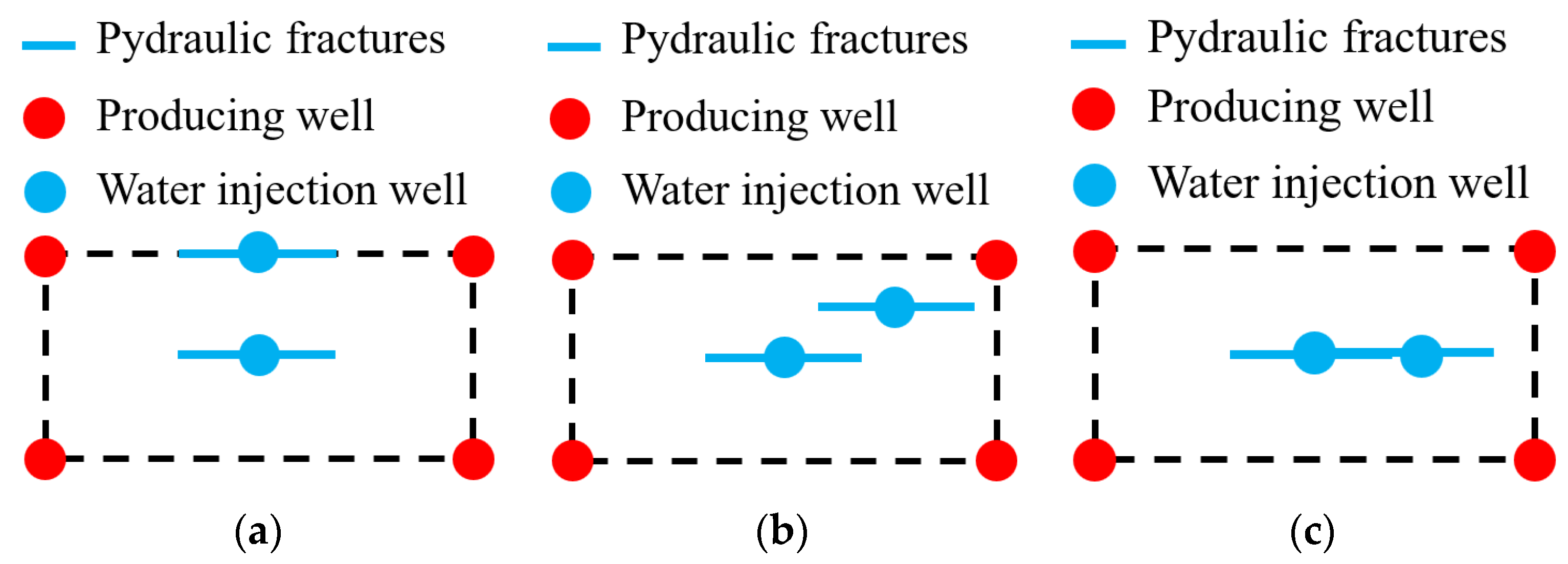
In the G block, characterized by low permeability, high crude oil viscosity, and significant spacing between oil and water wells, establishing an effective displacement system between these wells presents a considerable challenge. Consequently, experiments are essential to explore alternative development approaches. Hydraulic fracturing emerges as a viable option for exerting effective control over the reservoir. In the existing layout of the G experimental area, with well spacing set at 300 × 150 m, hydraulic fracturing can efficiently control the reservoir’s behavior along the fracture length but struggles to achieve effective control in the fracture width direction. Therefore, adjustments for well pattern enhancement become necessary.

As depicted in Figure 6, three well pattern enhancement schemes are employed for the five-spot well pattern. These schemes closely resemble the enhancement approach used for the inverted nine-spot well pattern. In Figure 6a, the first scheme focuses on enhancing same-row vertical well spacing. Unlike the inverted nine-spot well pattern, the newly added injection wells are positioned in the same column as the original injection wells but are oriented at a 90° angle to the fracture direction. The other two well pattern enhancement schemes involve 45° horizontal well spacing and 90° horizontal well spacing.

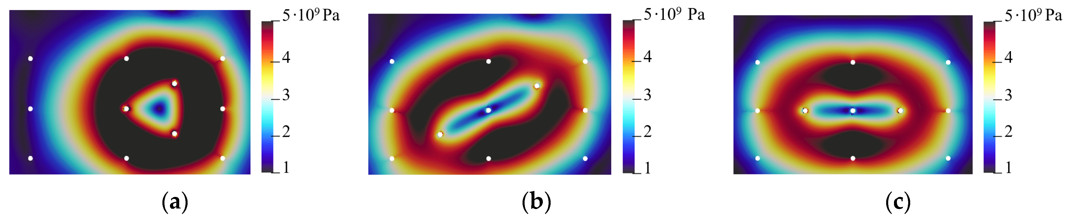
Based on the five-spot well pattern, simulations were conducted to assess the impact of different injection well enhancement schemes on the pressure-driven waterflooding development process, while keeping the daily injection rate constant (800 m³/d). The stress field distribution is shown in Figure 7. This analysis aimed to clarify the influence of various injection well enhancement schemes on the dynamics of pressure-driven waterflooding development. From the simulation results, it can be observed that in the five-spot well pattern: In the case of using the same column vertical well enhancement, as shown in Figure 7a, the four production wells experience relatively low stress levels. However, it is challenging to establish an effective drainage relationship between oil and water wells, resulting in overall low oil recovery. When using the 45° horizontal well spacing, as shown in Figure 7b, only the upper-right production well experiences a relatively high stress level, leading to effective water displacement. The well in the lower-right corner performs next best, while the two wells on the left side show poor oil recovery. In the case of using the 90° horizontal well spacing, as shown in Figure 7c, the two production wells on the right-side achieve effective water displacement, while the two wells on the left side exhibit slightly weaker water displacement effects. These findings emphasize the varying effects of different injection well enhancement schemes on the waterflooding efficiency and oil recovery in the five-spot well pattern.

A study was conducted on the impact of different well pattern enhancement schemes on the cumulative liquid production of the low-permeability reservoir. Figure 8 illustrates the correlation between the injection well enhancement scheme and the cumulative liquid production of oil wells within the five-spot well pattern. From the simulation results, it can be observed that under the same column vertical well enhancement scheme, the cumulative oil production is the lowest, and there are issues such as “low liquid, low production” in the oil wells. On the other hand, the 90° horizontal well spacing scheme exhibits exceptional performance, resulting in the highest cumulative liquid production among all schemes. It is clearly outperforming the other two well pattern enhancement schemes. In conclusion, within the G block, when implementing the five-spot well pattern, the 90° horizontal well spacing scheme stands out as the most effective choice, delivering superior results in terms of cumulative liquid production.

4.3. Inverted Nine-Spot Well Pattern Enhancement Scheme

As shown in Figure 9, three well pattern enhancement schemes are used for the inverted nine-spot well pattern: Figure 9a depicts the single-row wellbore spacing where wells are oriented at a 90° angle to the fracture direction. Figure 9b illustrates the 45° horizontal well spacing where wells are drilled at a 45° angle to the fracture direction. Figure 9c shows the 90° horizontal well spacing where wells are drilled horizontally in alignment with the fracture direction.

Based on the inverted nine-spot well pattern, simulations were conducted to study the impact of different injection well enhancement schemes on the pressure-driven waterflooding development process, while maintaining a constant daily injection rate (800 m³/d). The stress field distribution is shown in Figure 10. This analysis aimed to clarify the influence of various injection well enhancement schemes on the dynamics of pressure-driven waterflooding development.

From the simulation results in the inverted nine-spot well pattern, we can observe the following: When using the single-row wellbore spacing, as shown in Figure 10, the oil wells on the left side experience relatively low stress levels. However, it is challenging to establish an effective drainage relationship between oil and water wells, resulting in overall low oil recovery. With the 45° horizontal well spacing, as shown in Figure 10, waterflooding covers a broader range. Except for the oil wells in the upper-left and lower-right corners, the rest of the oil wells experience effective water displacement. When using the 90° horizontal well spacing, as shown in Figure 10, the stress around the injection wells is more evenly distributed, leading to effective water displacement for the surrounding oil wells. These observations highlight the different effects of various injection well enhancement schemes on the waterflooding efficiency and oil recovery in the inverted nine-spot well pattern.

To further clarify the mechanisms of enhanced oil recovery and water injection techniques with different wellfield densification methods, a study was conducted to investigate the impact of various wellfield densification schemes on the cumulative liquid production of low-permeability reservoirs. Figure 11 illustrates the relationship between the injection well densification method and the cumulative liquid production from oil wells in the inverted nine-spot well pattern. From the simulation results, it can be observed that when using the single-column vertical well densification scheme, as shown in Figure 11, the cumulative oil production is low. In contrast, the 45° horizontal well spacing performs the best, resulting in the highest cumulative liquid production, followed by the 90° horizontal well spacing. The results indicate that when the daily injection rate from water wells is 800 m³/d, different wellfield densification methods lead to varying degrees of damage and fracturing in the rock matrix, resulting in different improvements in reservoir properties. This, in turn, leads to variations in oil well liquid production. Therefore, in G Block, using the inverted nine-spot well pattern with 45° horizontal well densification significantly enhances waterflooding recovery and improves the effectiveness of waterflooding development for low-permeability reservoirs.

5. Evaluation Method Based on Percolation Field Variation

5.1. Indicator Reflecting Fluid Flow Capability

When the reservoir is a horizontal, isotropic formation, and the thickness of the oil layer is constant, the seepage velocity at any position on the reservoir plane can be calculated using the following equation:

$$v=-\frac{K}{\mu }grad(p)$$

(22)

When the permeability (K) and viscosity (μ) values in the formation are constants, the fluid seepage velocity is solely dependent on the pressure gradient at that location and exhibits a positive correlation. As the pressure gradient increases at a particular location, the fluid seepage velocity at that position also increases. Consequently, a higher fluid seepage velocity at a specific location indicates a stronger depleting capability and better reservoir exploitation performance. Thus, the reservoir exploitation performance at a certain location can be characterized by the pressure gradient at that location.

Through the study of the combined well network seepage model under different horizontal wellbore spacing methods, the potential function distribution for various horizontal wellbore spacing approaches was obtained. By establishing the relationship between the potential function and pressure in the seepage field, the pressure gradient at any point in the planar seepage field can be determined.

$$d\varphi =\frac{K}{\mu }dp$$

(23)

The pressure, P(i, j), obtained through the potential function can be used to define the expression for the horizontal pressure gradient, ∇P_x, at any point on the plane as follows:

$$\begin{array}{l}\nabla P_x=\frac{P(i,j)-P(i,j-1)}{dx}\\ i=1,2,\dots N;j=2,3,\dots N\end{array}$$

(24)

The expression for the vertical pressure gradient, ∇P_y, on the plane is defined as follows:

$$\begin{array}{l}\nabla P_y=\frac{P(i,j)-P(i,j-1)}{dy}\\ i=2,3,\dots N;j=1,2,\dots N\end{array}$$

(25)

Here, ∇P_x and ∇P_y are vectors, and their numerical values are obtained through the above equations. The horizontal pressure gradient is in the direction of the x-axis, and the vertical pressure gradient is in the direction of the y-axis. The total driving pressure gradient, ∇P, at any point in the reservoir can be obtained by superimposing the horizontal and vertical pressure gradients. The expression is as follows:

$$\nabla P=\sqrt{\nabla P_x{}^2+\nabla P_y{}^2}$$

(26)

The total driving pressure gradient at any point in the reservoir reflects the fluid’s flow capability at that location. It can be used to assess the exploitation potential at that location. When the total driving pressure gradient at a specific location is higher, the fluid seepage velocity at that point is also higher, indicating a stronger fluid flow capability and greater reservoir exploitation potential at that location.

5.2. Characterization of Exploitation Effectiveness in Injection and Production Units

(1)

Dimensionless Exploitation Range, S_Di, in the Injection and Production Unit

Let S₀ be the control area of a typical injection and production well network unit. In the injection and production unit, the area enclosed by the contour lines of equal pressure gradient for a specific value i is the exploitation range Si corresponding to that pressure gradient.

To eliminate the influence of absolute data sizes, the dimensionless exploitation range S_Di is defined as:

$$S_{Di}=\frac{S_i}{S_0},(0<S_{Di}<1)$$

(27)

The dimensionless exploitation range value, S_Di, reflects the range occupied by a specific pressure gradient value within the control area of the injection and production unit well network. When the dimensionless exploitation range of high displacement pressure gradient values is larger, it signifies a larger area of high-speed exploitation within the well network unit. This characterization indicates a more effective exploitation of reservoir reserves in that well network unit.

(2)

Surface Displacement Intensity, S_d, in the Injection and Production Unit

The surface displacement intensity, S_d, is defined to characterize the exploitation effectiveness in the well network. Its definition is given by:

$$S_d={\displaystyle \sum S_{Di}\times \nabla p_i}$$

(28)

A higher value of surface displacement intensity, S_d, in the reservoir well network unit indicates a greater driving force within the dimensionless exploitation range under current conditions, implying a more effective exploitation of reservoir reserves within the well network unit. The unit is MPa/m. It is possible to quantitatively analyze the seepage field of the combined well network, plot the variation curve of surface displacement intensity S_d under different conditions, and analyze the impact of different factors on the effective exploitation of reserves.

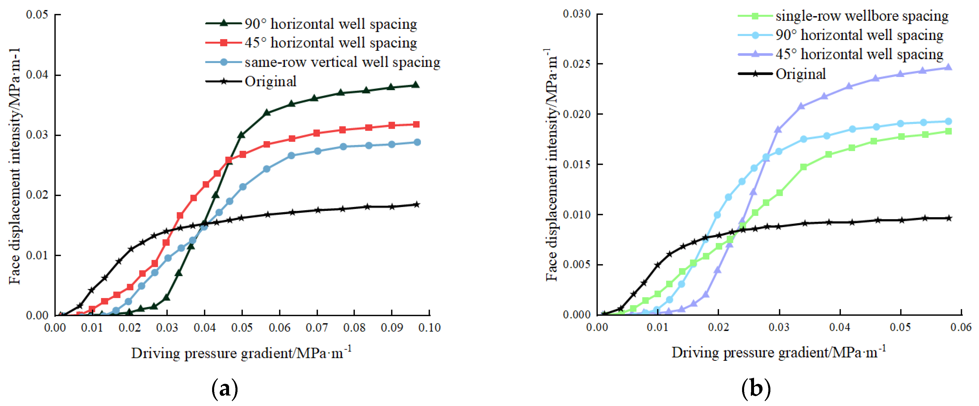
5.3. Comparison of Injection and Production Seepage Fields with Different Horizontal Wellbore Spacing Methods

Using the established reservoir exploitation effectiveness evaluation method, the dimensionless exploitation range of combined well networks formed by different horizontal wellbore spacing methods was calculated under the basic reservoir conditions. The influence of deploying horizontal wells on the exploitation effectiveness of the base vertical well network was analyzed. The results are shown in Figure 12 and Figure 13.

From the figures, it is evident that the inter-well exploitation and reservoir exploitation effectiveness of the injection and production well network unit have undergone certain changes after deploying horizontally spaced wells. Comparing the dimensionless exploitation range of different combined well networks, it can be concluded that a smaller high-speed flow area indicates a smaller and less effective region for reservoir exploitation in this well network configuration. The deployment of horizontal wells effectively increases the degree of reservoir exploitation in the well network. Comparing the inter-well exploitation effectiveness of different well networks, it can be observed that the five-point method with 90° horizontal well spacing and the nine-point method with 45° horizontal well spacing yield the best adjustment effects, as evidenced by the statistical calculation of the surface displacement intensity under various well network conditions.

6. Research on Timing of Water Injection in Pressure-Driven Water Flooding

In Section 4 of our research, we discovered that for the five-spot pattern, the 90° horizontal well spacing yielded the highest daily oil production, while for the nine-spot pattern, the 45° horizontal well spacing was the most effective. Therefore, in this section, based on the five-spot pattern with 90° horizontal well spacing and the nine-spot pattern with 45° horizontal well spacing, we further investigate the changes in daily and cumulative oil production under different timing scenarios for pressure-driven water flooding. Figure 14a,b illustrate the temporal variations in cumulative oil production for these two scenarios under pressure-driven water flooding (with an injection rate maintained at 800 m³/d). The numerical simulation results reveal that for the five-spot pattern with 90° horizontal well spacing, compared to pressure-driven water flooding after 90 days, conducting pressure-driven water flooding after 40 days increases cumulative oil production by 9.48% and reduces the average daily decline rate by 0.19%. Similarly, for the nine-spot pattern with 45° horizontal well spacing, initiating pressure-driven water flooding after 40 days, rather than 90 days, results in an 8.97% increase in cumulative oil production and a 0.18% decrease in the average daily decline rate. This underscores the significance of commencing pressure-driven water flooding at an earlier stage, facilitating rapid reservoir capacity replenishment, maintaining elevated reservoir pressure levels, and establishing an effective pressure displacement system. These factors collectively contribute to higher initial oil production rates and a slower rate of production decline, ultimately enhancing overall oil recovery.

7. Discussion

The finite discrete element method (FDEM), proposed in 1995 [27], is employed in this study to simulate the transition from a continuous medium to a discontinuous one. This method combines the advantages of the finite element method (FEM) for solving solid deformations and the discrete element method (DEM) for handling contact between blocks or two discontinuous surfaces. Additionally, FDEM incorporates the benefits of cohesive element models in simulating fracture propagation. Therefore, FDEM proves to be a suitable approach for modeling rock fractures. In this research, a detailed analysis of the relationship between fracture time and crack length was conducted. Numerical simulation results obtained through FDEM were extensively compared with the theoretical solutions of the classic KGD [28] model. The high consistency between numerical simulation results and theoretical analytical models indicates that FDEM accurately captures the morphology and characteristics of internal fracture propagation during water flooding development. It demonstrates the ability to reflect the magnitude of hydraulic pressure and accurately monitor oil and gas production after pressure drive. In the context of wellbore encryption for water injection, different approaches using the five-spot and reverse nine-spot methods significantly enhance oil and gas production from the reservoir. We conducted in-depth studies on three encryption wellbore methods under these two approaches, analyzing water pressure and oil and gas production while comprehensively evaluating reservoir depletion effects. The research findings suggest that employing encrypted water injection wells can effectively increase oil and gas production to a certain extent. This aligns with previous studies by Wang [29], Yang [30], and Xiang [31], indicating the positive impact of encrypted water injection wells on production enhancement. It is noteworthy that various scholars have proposed different encryption methods considering variations in the distribution of oilfield well networks. Despite the diversity of these approaches, they collectively contribute to increased oil and gas production to varying degrees. Through simulation studies and discussions, we can derive the most suitable water injection well encryption scheme for the current oilfield well network. 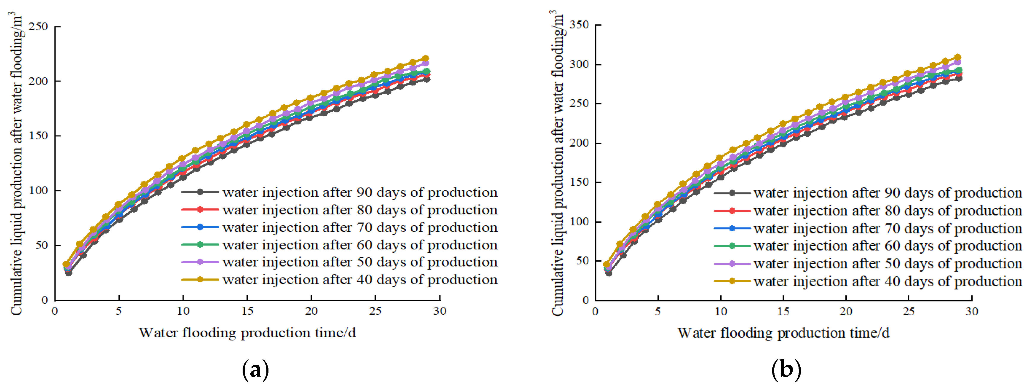In the investigation of water drive pressure displacement, our observations align with the results of Cha et al.’s [32] study. The research indicates that initiating water flooding in the early stages is beneficial for rapidly and effectively replenishing reservoir capacity, thereby maintaining a higher reservoir pressure level. Early implementation of water drive contributes to establishing an efficient pressure displacement system, resulting in higher initial oil well production and a slower decline rate, ultimately achieving better oil recovery rates. While drilling costs are relatively high, the investment is deemed necessary when compared to the lower associated costs of volume fracturing for late-stage water injection and oil well operations. The expenses for late-stage production increase relatively lower, but this investment brings greater value in terms of oil and gas resources. Therefore, early implementation of water drive, despite higher initial costs, can lead to more effective production increases in the later stages, enhancing the economic benefits of resource development. Overall, this strategy not only aids in maintaining a favorable reservoir condition but also creates more sustainable economic benefits throughout the entire development process.

8. Conclusions

In this study, a numerical simulation method for pressure-driven water injection in low-permeability reservoirs in the G test area is developed. The accuracy of our model was rigorously validated, successfully capturing the initiation and propagation of fractures during pressure-driven water injection. Our research focused on the five-spot pattern and the reverse nine-spot pattern, examining how varying wellbore spacing and orientations influenced the efficiency of water flooding in production wells. Additionally, we explored the repercussions of different wellbore spacing and orientations on cumulative liquid production. Lastly, we delved into the changes in cumulative oil production across diverse water injection timing scenarios.

• The FDEM method demonstrates excellent capabilities in simulating the initiation and propagation of fractures during pressure-driven water injection processes and allows for the optimization design of pressure-driven parameters.
• Among the different wellbore spacing and orientation strategies, it was observed that the five-spot pattern with a 90° horizontal wellbore spacing, derived from the five-point pattern, delivered the most favorable outcomes, boasting a cumulative liquid production approximately 32.32% higher than that of the same-column horizontal well spacing. Similarly, the reverse nine-spot pattern with a 45° horizontal wellbore spacing, based on the reverse nine-spot pattern, showed the best performance, with a cumulative liquid production approximately 30% higher than that of a single-column horizontal well spacing.
• Based on the varying distribution of pressure gradients within different well networks, an evaluation method for inter-well exploitation capability and its effectiveness was developed. This method allows for the quantitative assessment of reservoir exploitation under different horizontal wellbore spacing configurations. Notably, the adjustment effect was found to be most effective in the case of the five-point method with 90° horizontal well spacing and the nine-point method with 45° horizontal well spacing.
• Regarding the timing of pressure-driven water injection, for the five-spot pattern with 90° horizontal well spacing, compared to water injection after 90 days, injecting water after 40 days of production led to an increase in cumulative oil production of 9.48% and a reduction in the average daily decline rate of 0.19%. In the case of the reverse nine-spot pattern with 45° horizontal well spacing, injecting water after 40 days of production resulted in an 8.97% increase in cumulative oil production and a decrease in the average daily decline rate of 0.18%. This indicates that initiating pressure-driven water injection earlier can rapidly and effectively replenish reservoir capacity, maintaining a high reservoir pressure level.
• In the context of pressure-driven water injection development, this method plays a pivotal role in preserving or even increasing reservoir pressure. This, in turn, empowers oil wells to sustain higher production rates, decelerates the pace of production decline, extends the operational life of oil and gas fields, and facilitates the extraction of additional oil and gas resources.