Machine Learning Aided Prediction of Glass-Forming Ability of Metallic Glass

Abstract

The prediction of the glass-forming ability (GFA) of metallic glasses (MGs) can accelerate the efficiency of their development. In this paper, a dataset was constructed using experimental data collected from the literature and books, and a machine learning-based predictive model was established to predict the GFA. Firstly, a classification model based on the size of the critical diameter (D_max) was established to determine whether an alloy system could form a glass state, with an accuracy rating of 0.98. Then, regression models were established to predict the crystallization temperature (T_x), glass transition temperature (T_g), and liquidus temperature (T_l) of MGs. The R² of the prediction model obtained in the test set was greater than 0.89, which showed that the model had good prediction accuracy. The key features used by the regression models were analyzed using variance, correlation, embedding, recursive, and exhaustive methods to select the most important features. Furthermore, to improve the interpretability of the prediction model, feature importance, partial dependence plot (PDP), and individual conditional expectation (ICE) methods were used for visualization analysis, demonstrating how features affect the target variables. Finally, taking Zr-Cu-Ni-Al system MGs as an example, a prediction model was established using a genetic algorithm to optimize the alloy composition for high GFA in the compositional space, achieving the optimal design of alloy composition.

1. Introduction

Solid-state structure can be categorized into crystalline, quasi-crystalline, and amorphous states based on the arrangement of particles. Crystalline structures exhibit a regular and ordered arrangement of particles in three-dimensional space, demonstrating long-range order and translation symmetry. These structures possess lower energy and higher stability, which explains why most everyday solid materials showcase crystalline structures. Quasi-crystalline structures, on the other hand, possess long-range orientational order but lack long-range translational order. Amorphous structures, characterized by a lack of ordered particle arrangements, do not exhibit periodicity or translational symmetry. Although they exhibit short-range order, they display long-range disorder. Metallic glass (MGs) serves as a typical example of amorphous materials. Due to the unique particle arrangement in MGs, which is less susceptible to lattice defects, they possess exceptional properties that are not commonly found in crystalline structures. These properties include high strength [1], high wear resistance [2], high elastic limits [3], corrosion resistance [4], and excellent soft magnetic properties [5]. Consequently, MGs hold vast potential for numerous applications. However, the glass-forming ability (GFA) of MGs plays a crucial role in limiting their application as conventional materials. The GFA refers to a metal’s ability to form an amorphous glassy state during the cooling process. A higher GFA indicates a greater ease of achieving the amorphous state, resulting in improved processability and performance enhancements.

The prediction of GFA plays a crucial role in understanding the behavior of MGs, particularly in investigating the impact of composition on the GFA. Traditionally, research on GFA has primarily focused on experimentation, where the GFA is obtained by adjusting the composition of MGs. This approach heavily relies on empirical knowledge and experience. However, the process of finding MGs with high GFA through trial and error can be time-consuming and resource intensive. To address this challenge, machine learning approaches have gained significant attention in the field of GFA. By leveraging large amounts of experimental data, machine learning techniques have been applied to analyze and predict the GFA of MGs. These approaches enable researchers to develop models that can accurately predict the GFA of new compositions, thereby reducing the need for extensive experimentation. Currently, most GFA predictions are based on estimating the critical diameter (D_max) [6,7,8,9,10,11,12,13]. While D_max provides a direct measure of GFA, it is influenced by various factors, including fabrication processes, sample shape, and testing methods. Consequently, even MGs with identical compositions can exhibit significant variations in D_max, resulting in low prediction accuracy when developing models. This limitation impedes the wider application of machine learning in the field of metallic glasses. Researchers have discovered strong correlations between the GFA and the crystallization temperature (T_x), glass transition temperature (T_g), and liquidus temperature (T_l) of MGs, which can be reliably measured using thermal analysis techniques. T_x refers to the temperature at which a material transitions from a solid or amorphous state to a crystalline state. T_g represents the temperature below which an amorphous material, such as glass or a polymer, becomes rigid or solid-like. This is the point where the material transitions from a supercooled liquid to a glassy state. T_l refers to the temperature at which a substance completely melts and turns into a liquid phase. It is the highest temperature at which both solid and liquid phases coexist in equilibrium. Therefore, it is reasonable to explore alternative parameters that can capture GFA as a composite of these temperature-related properties, thus overcoming the limitations associated with D_max. Turnbull et al. [14] introduced the reduced glass transition temperature (T_rg = T_g/T_l) based on the crystallization kinetics of supercooled liquids as a way to characterize GFA. Higher T_rg values are indicative of greater GFA. Chen et al. [15] and Inoue et al. [16] proposed that the supercooled liquid region (ΔT_x = T_x − T_g) of MGs reflects the stability of the supercooled liquid, and can thus serve as a measure of the GFA. Lu et al. [17] combined T_rg and ΔT_x to introduce a novel GFA parameter γ, where γ = T_x/(T_g + T_l). Experimental results have demonstrated that γ is an effective indicator of the GFA.

These studies suggest that parameters like T_x, T_g, and T_l are effective indicators of the GFA of MGs. However, there is currently limited research focused on predicting these temperature parameters. In this study, we gathered a substantial amount of the GFA data for MGs from literature sources and utilized machine learning techniques to develop predictive models. Furthermore, we conducted feature selection and interpretability analysis to identify the key factors influencing these parameters. We proposed composition strategies to enhance the GFA of MGs and combined them with a genetic algorithm to explore novel MGs. These findings provide valuable insights for the future design of MGs.

2. Materials and Methods

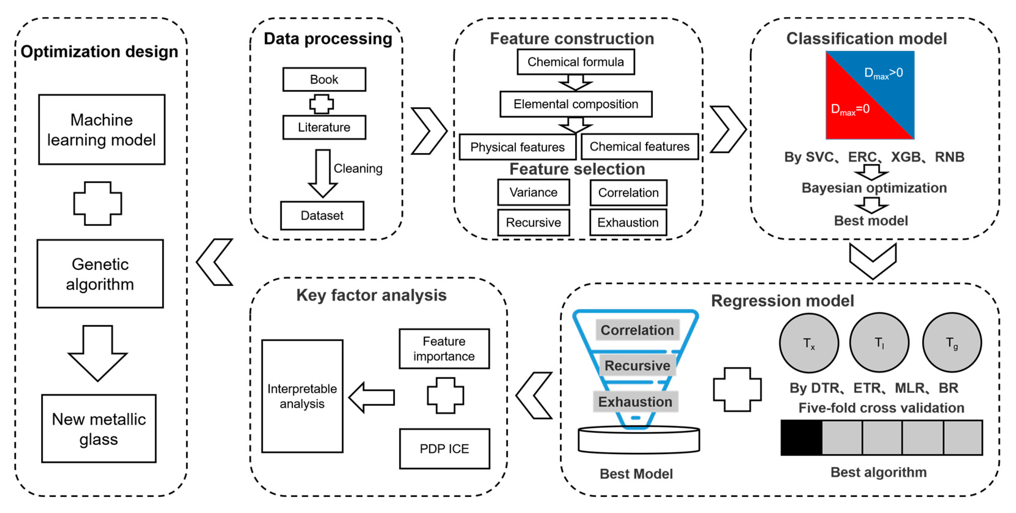
2.1. Machine Learning Model Framework

In this study, a machine learning-based prediction model was developed to estimate the GFA of MGs. This study aimed to investigate the impact of key feature variables on GFA, providing theoretical and model support for optimizing and designing MG compositions. The research process followed a specific framework, as illustrated in Figure 1. The framework involved several steps, including data processing, feature construction, construction of classification and regression models, analysis of key factors, and optimization design. During the data processing phase, a comprehensive dataset was compiled by collecting D_max, T_x, T_g, and T_l values of different alloy compositions from the literature and books. The chemical formulas of the alloys were then transformed into machine-learning-friendly features through careful feature construction. These transformed features were utilized to establish a classification model to determine whether D_max was greater than 0. For alloys with D_max greater than 0, separate regression models were developed to predict T_x, T_g, and T_l. To further refine the models, feature selection techniques were employed to simplify and optimize their performance. Finally, a synergistic combination of the predictive models and a genetic algorithm was utilized to explore the compositional space and identify novel alloys with high GFA.

2.2. Dataset Establishment

The dataset used in this study was primarily compiled by Ward et al. [18] and included experimental data on the GFA of MGs up until 2018. The data were sourced from books [19] and the literature [20,21,22,23,24,25,26,27,28,29]. Subsequently, additional experimental data published from 2018 to the present [10,12,30,31,32,33,34,35,36,37,38,39,40,41,42,43,44,45,46,47,48,49,50,51,52,53,54,55,56,57,58,59,60,61,62,63,64,65] were collected and incorporated into the dataset. This combination of sources formed the basis of the new dataset for this study. Figure 2 shows the distribution of elements contained in the data set in the periodic table of elements. The dataset primarily consists of the chemical formulae of MGs and their corresponding D_max, T_l, T_x, and T_g. The sample quantities for D_max, T_l, T_x, and T_g are 10,194, 751, 791, and 846, respectively.

2.3. Feature Construction and Selection

Given that the dataset solely considers the impact of chemical formulas on the GFA, the process of feature construction primarily revolves around the composition of MGs. Firstly, the chemical formulas are transformed into elemental compositions. Subsequently, the physical and chemical properties of each element are taken into consideration, and a weighted average is computed based on the elemental composition, as shown in

Table 1. Feature name and description.

Feature Name	Description	Feature Name	Description
Number	Atomic number	N(s,p,d,f) valence	Number of electrons in (s,p,d,f) level
Mendeleev number	Mendeleev number	N(s,p,d,f) unfilled	Number of unfilled electrons in (s,p,d,f) energy level
Atomic weight	Atomic weight	N unfilled	Number of unfilled energy layer electrons
Melting temperature	Melting point	GS volume_pa	Average volume of atoms
Column	Column of the element	GS bandgap	Band gap of elements
Row	Row of the element	GS magmom	Magnetic moment of element
Covalent radius	Covalent bond radius	Space group number	Group serial number
Electronegativity	Electronegativity of elements	N valence	Energy layer electron number

. Moreover, in order to enhance the dimensionality of the features and mitigate overfitting [66], statistical features, such as the maximum value, minimum value, and absolute deviation of elemental properties, are incorporated. This results in the generation of 132 descriptors, which collectively form the input data for forecasting the GFA.

To identify the key features that influence the GFA of MGs, it is essential to conduct feature selection on the constructed dataset. Firstly, a variance filter is applied to identify and eliminate features with low variances. Subsequently, F-tests [67] are utilized to detect and remove highly correlated features. Additionally, an embedding method [68] is employed to further refine the feature selection process. This method evaluates the contribution of each feature to the model by assigning weights during training and automatically eliminates features with low importance below a predefined threshold. Following the embedding method, a recursive feature elimination [69] technique is used to iteratively remove features. The criterion of threshold selection in the embedding method is to increase the threshold and reduce the number of features of the model without affecting the accuracy of the model as much as possible. The recursive method constructs different feature subsets to train the model, uses MAE as the evaluation index of the model, and gradually selects the features that are beneficial to the model performance, thus realizing the feature selection. The criterion of feature number selection in recursion is that when the number of features continues to increase, the accuracy of the model does not improve, and it is considered that this is the best feature number. This iterative process effectively reduces the dimensionality of the features. Finally, an exhaustive search [70] is conducted on the remaining features to identify the key features that significantly influence the GFA. The exhaustive method is to combine the features selected by the recursive method, select R² and MAE as evaluation indexes, calculate the performance of the model under various combinations, and obtain the best performance feature combination.

2.4. Machine Learning Model and Feature Analysis

The construction of the machine learning model involves two main steps. Firstly, the classification stage uses D_max > 0 or D_max = 0 as the criterion, and commonly used classification algorithms such as Support Vector Machine (SVC), Extremely Randomized Trees (ETC), XGBoost (XGC), and Naive Bayes (GNB) are applied to determine whether an alloy’s composition can be transformed into Bulk Metallic Glasses (BMGs). Then, in the regression stage, regression algorithms, including Decision Tree Regression (DTR), Extremely Randomized Trees Regression (ETR), Multi-layer Perceptron Regression (MLP), and Linear Regression (LR), are employed to analyze the characterization parameters of BMGs’ GFA. This aims to establish a predictive model that can estimate the relationship between composition and GFA. The data set is divided into the training set and test set according to 8:2. The training set is used to train the model, and the subsequent test set is used to verify the generalization ability of the model. In the comparison of regression algorithms, in order to avoid the problem of under-fitting or over-fitting models caused by randomly dividing training data, K-fold cross-validation is used to calculate the evaluation indexes of different models [71,72]. K-fold cross-validation involves dividing the dataset into k subsets, using k-1 subsets for training and one subset for testing in each iteration. The model is then run k times, and the average of the k results is considered the final evaluation metric. In this study, a five-fold cross-validation approach was adopted to ensure reliable model performance assessment.

For different machine learning models, classification and regression tasks require the use of different evaluation metrics. In the case of classification models, particularly binary classification models, the performance is typically assessed using a confusion matrix. The values within the confusion matrix [73] represent the model’s classification predictions and include True Positive (TP), False Positive (FP), True Negative (TN), and False Negative (FN), as shown in

Table 2. The confusion matrix of binary classification.

Actual	Predicted
	Positive	Negative
Positive	TP	FN
Negative	FP	TN

. These values enable the calculation of various evaluation metrics, including Accuracy, Precision, Recall, and F1 score. The formulas for these metrics are presented in Equations (1)–(4).

$$\mathrm{Accuracy}=\frac{TP+TN}{TP+FN+FP+TN}.$$

(1)

$$\mathrm{Precision}=\frac{TP}{TP+FP}$$

(2)

$$\mathrm{Recall}=\frac{TP}{TP+FN}$$

(3)

$$\mathrm{F}1=\frac{2\times \mathrm{Precision}\times \mathrm{Recall}}{\mathrm{Precision}+\mathrm{Recall}}$$

(4)

In order to further assess the effectiveness of different classification models, the Receiver Operating Characteristic (ROC) curve was employed to compare their generalization ability. The ROC curve illustrates the relationship between the TP and the FP of a classifier. In the ROC curve, the FP is plotted on the horizontal axis, and the TP is plotted on the vertical axis. Each point on the ROC curve corresponds to the TP and FP values obtained at a specific threshold used for classification. A classifier with a ROC curve closer to the top-left corner demonstrates better performance. Moreover, the area under the ROC curve serves as an indication of the model’s performance, with a larger area suggesting better performance.

For regression models, evaluating the performance involves comparing the predicted values with the actual values. As such, Mean Squared Error (MSE), Mean Absolute Error (MAE), and Coefficient of Determination (R-squared, R²) serve as common evaluation metrics to assess the accuracy of the model. The formulas for these metrics are presented in Equations (5)–(7).

$$MSE={\displaystyle \sum _{i=1}^n\frac{1}{n}}{({\hat{y}}_i-y_i)}^2.$$

(5)

$$MAE={\displaystyle \sum _{i=1}^n\frac{1}{n}}\left|{\hat{y}}_i-y_i\right|$$

(6)

$$R^2=1-\frac{{\displaystyle \sum _{i=1}^n{({\hat{y}}_i-y_i)}^2}}{{\displaystyle \sum _{i=1}^n{(\overline{y_i}-y_i)}^2}}$$

(7)

where y_i represents the actual value, ȳ_i represents the average of the actual values, and ŷ_i represents the predicted value. MAE and MSE measure the gap between the predicted and actual values, with a smaller value indicating smaller prediction errors. The R² quantifies the level of fit between the predicted and actual values. A value closer to 1 implies a better fit between the predictions and the actual values.

Most machine learning models are often considered black box models, as they can establish the mapping between input features and output results without providing explicit expressions. This lack of interpretability is a common issue. To address this, the current paper introduces Partial Dependence Plots (PDP) and Individual Conditional Expectation Plots (ICE) [74,75,76,77]. The fundamental concept underlying PDP is to assess the impact of a single feature on the output while keeping the other features constant. This analysis helps reveal the nonlinear relationships present in the model’s output. PDP is based on a straightforward observation: in many cases, the model’s output depends not solely on the value of an individual variable but rather on the simultaneous changes in the combination of different variables. By simplifying this multivariate relationship, PDP can effectively describe the effect of a single feature on the model’s output. Conversely, ICE plots are primarily employed to illustrate the relationship between the variable values of individual samples and their corresponding response values. ICE plots effectively reveal the nonlinear relationships and trends within the model’s output. The calculation of ICE plots involves determining the changes in the model’s predicted output for each individual sample as the feature values vary. The x-axis represents the arrangement of individual variable values, while the y-axis represents the predicted output for each sample. For each feature value, ICE plots visually capture the nonlinear changes in the specific feature by plotting the response values for each individual sample within a single graph.

2.5. Composition Optimization

Due to the huge search space, it is unrealistic to use enumeration to find the best point, so genetic algorithm is used to optimize the composition. NSGA-II [78,79] is a classic multi-objective optimization algorithm based on genetic algorithms. NSGA-II evaluates and selects individuals using non-dominated sorting and crowding distance to solve multi-objective optimization problems. The basic principles of the NSGA-II algorithm are as follows: Non-dominated Sorting, Crowding Distance Assignment, Selection, Crossover, Mutation, and Termination. The NSGA-II algorithm combines non-dominated sorting and crowding distance to find a set of non-dominated solutions in multi-objective optimization problems while maintaining the diversity and convergence of the population. This algorithm has the ability to maintain a diverse set of solutions and explore the solution space effectively. The non-dominated sorting ensures that the algorithm can find a balance between different objectives, rather than just searching for a single optimal solution. The crowding distance is used to measure the density of individuals within each non-dominated level, reflecting the distribution of individuals in the objective space. By considering both non-dominated sorting and crowding distance, the NSGA-II algorithm is able to maintain a diverse population and avoid converging to local optima. This algorithm has been widely used and was proven to be effective in various applications.

3. Results

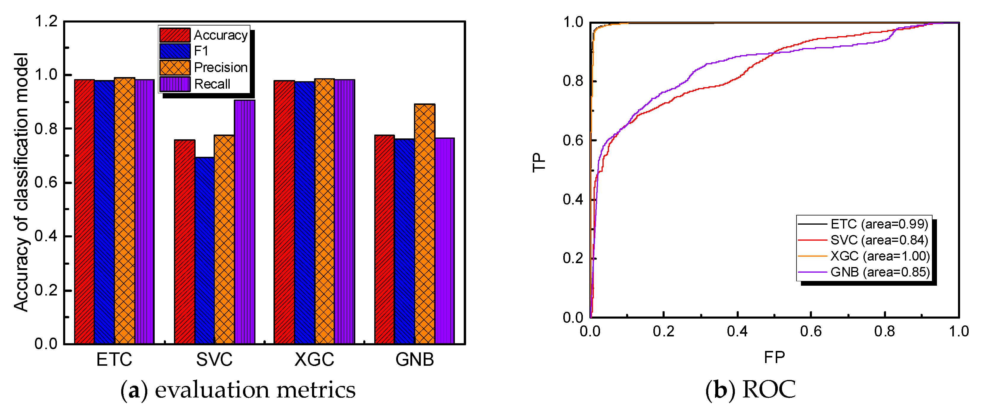
3.1. Classification Model Evaluation and Feature Selection

Figure 3 shows the performance comparison of four classification models. Figure 3a shows a comparative analysis of four classification models in terms of performance metrics. The ETR and XGC models demonstrate superior performance compared to the SVC and GNB models. Both the ETR and XGC models exhibit accuracy, precision, recall, and F1-score values above 0.98, indicating their high accuracy in classifying various labels. Furthermore, Figure 3b shows an examination of the ROC curves for the four models, revealing that the ETC and XGC models yield curves positioned more towards the upper-left corner, encompassing larger areas. The ETC model has an enclosed area of 0.99, while the XGC model achieves a perfect score of 1. This signifies the superior performance of both models compared to XGC. Consequently, the XGC model was selected for the subsequent development of the classification model.

3.2. Regression Model Evaluation and Feature Selection

This study investigated the GFA of BMGs using three characterization parameters: T_l, T_g, and T_x. Multiple machine learning algorithms were applied to predict these parameters, and a five-fold cross-validation method, similar to the previous evaluation, was employed for performance assessment. Figure 4 shows the performance of T_l, T_g, and T_x on different regression models. It can be observed that among the four regression models, the ETR model exhibits the highest R² and the lowest MSE and MAE. Overall, the results indicate that the ETR model demonstrates the best performance, and therefore, it was selected for subsequent predictions. Figure 5 compares the predicted and experimental values of T_l, T_g, and T_x using the ETR model. The predicted values closely align with the diagonal line, indicating excellent accuracy of the model predictions. At the test set: the R² of T_l reaches 0.98, with a MAE of 23.21 K and a MSE of 1481.73 K². For T_g, the R² is 0.89, with a MAE of 22.72 K and a MSE of 3786.02 K². As for T_x, the R² is 0.98, with a MAE of 12.19 K and a MSE of 413.13 K².

Table 3. GFA parameters and corresponding prediction accuracy.

No	Criteria	Formula	R2	Ref.
1	Trg	Trg = Tg/Tl	0.24168	[80]
2	δ	δ = Tx/(Tl − Tg)	0.34638	[81]
3	βr	βr = (TxTg)/(Tl − Tx)2	0.45692	[82]
4	w	w = Tl(Tl + Tx)/[Tx(Tl − Tx)]	0.48693	[83]
5	ΔTx	ΔTx = Tx − Tg	0.44805	[16]
6	γ	γ = Tx/(Tg + Tl)	0.50375	[17]
7	βl	βl = Tx/Tg + Tg/Tl	0.51967	[84]
8	γm	γm = (2Tx − Tg)/Tl	0.52861	[85]
9	υ	υ = TxTg(Tx − Tg)/(Tl − Tx)3	0.59435	[86]
10	wB	wB = (2Tx − Tg)/(Tl + Tx)	0.53842	[87]
11	γc	γc = (3Tx − 2Tg)/Tl	0.55126	[88]
12	γn	(5Tx − 3Tg)/Tl	0.26394	[89]
13	w1	Tg/Tx − 2Tg/(Tg + Tl)	0.24006	[24]
14	χ	χ = [(Tx − Tg)/(Tl − Tx)][Tx/(Tl − Tx)]1.47	0.60217	[90]
15	Gp	Gp = Tg(Tx − Tg)/(Tl − Tx)2	0.5999	[6]
16	Dmax	-	0.70566	[9]
17	Dmax	-	0.795	[91]

presents the calculation formulas and corresponding prediction accuracies of the previous studies related to the GFA parameters. Two categories of GFA parameters were identified: the direct use of D_max and mixed mathematical expressions involving T_l, T_g, and T_x. However, both approaches yield relatively low prediction accuracies. In contrast, this study achieved R² values greater than 0.91 for T_l, T_g, and T_x predictions. Therefore, utilizing this study’s method to predict T_l, T_g, and T_x followed by corresponding parameter calculations can effectively enhance the prediction accuracy.

In order to simplify the model and identify the key features that affect the GFA, it is necessary to perform feature selection on the input features of the model. Figure 6 illustrates the process of feature selection for three representative parameters: T_l, T_x, and T_g. Each parameter’s input features are subjected to variance filtering, correlation filtering, embedded method filtering, recursive filtering, and exhaustive filtering. This gradual process of dimensionality reduction ensures that the model’s accuracy is not compromised. The changes in feature dimensionality throughout this process are depicted in Figure 7. After applying these dimensionality reduction methods, the input feature dimensions for all three parameters are reduced to 4, greatly simplifying the model. Additionally, the key features that significantly influence the GFA are identified and presented in

Table 4. The key features after screening.

	Key Feature	Description
Tl	Mean GSvolume_pa	Mean atomic volume
	Mean Electronegativity	Average electronegativity of elements
	Mean Gsmagmom	Average magnetic moment of elements
	Avg_dev MendeleevNumber	Average deviation of Mendeleev number
Tx	Mean Electronegativity	Average electronegativity of elements
	Avg_dev MendeleevNumber	Average deviation of Mendeleev number
	Mean GSvolume_pa	Mean atomic volume
	Mean NdUnfilled	Average orbital number of electrons in d layer that are not filled
Tg	Mean MeltingT	Average melting point of elements
	Mean Column	Mean column of elements
	Mean Gsmagmom	Average magnetic moment of elements
	Mean NdUnfilled	Average orbital number of electrons in d layer that are not filled

. These features can be broadly categorized into two classes: basic properties, such as melting point, volume, column, and Mendeleev Number, as well as electronic characteristics, such as electronegativity, unfilled electron number, and magnetic moment.

Analyzing the selected features can provide insight into their impact on the target variable. After several decades of research on MGs, researchers have identified several principles that contribute to improving the GFA, including the Inoue empirical rules [16], the similar atom substitution principle [92], and the electron concentration principle [93,94]. According to the Inoue empirical rules, the formation of MGs with high GFA should follow three principles: (1) the alloy system should consist of three or more elements; (2) the atomic size difference between the primary alloy components should exceed 14%; (3) and the mixing enthalpy between the primary composition elements in the alloy system should be negative. These rules indicate that the GFA is linked to the composition of elements, atomic size, and mixing enthalpy. On the other hand, the Miedema model [95,96] establishes relationships between the basic properties of elements (e.g., melting point, volume, column) and these parameters, providing partial insights into the GFA. The electron concentration principle proposes criteria for determining equivalent electron concentration, while electronic characteristics, such as electronegativity, unfilled electron number, and magnetic moment, can effectively explain variations in electron concentration, thereby influencing the GFA.

3.3. Analysis of Key Features

(1)

Feature importance analysis

In order to comprehend the impact of features on the ultimate target value, an analysis was performed to determine the importance of each feature in the established prediction model, as illustrated in Figure 8. The results indicated that the average orbital number of electrons in d layer that are not filled, the average atomic volume, and the average electronegativity emerged as the most significant features for T_g, T_x, and T_l, respectively. Consequently, when devising the composition of MGs, these features should be given particular consideration.

(2)

Analysis of PDP and ICE plots

In order to provide a more visually informative illustration of how these features impact the target value, we utilized PDP and ICE plots for feature analysis. The PDP plot showcases the influence of a single variable on the average target value. Figure 9 shows the PDP plot analysis of key features versus T_l. As Mean GSvolume_pa increases, T_l consistently decreases, with a brief spike when Mean GSvolume_pa reaches 20, followed by a continued decline. Conversely, T_l increases steadily as Mean electronegativity rises until it reaches 1.8, after which, Tl begins to decline. Figure 9c shows the combined effect of Mean GSvolume_pa and Mean electronegativity on T_l. Specifically, T_l tends to be smaller when Mean GSvolume_pa ranges from 25 to 28 and Mean electronegativity ranges from 1.3 to 1.4. Conversely, T_l tends to be larger when Mean GSvolume_pa ranges from 12 to 13 and Mean electronegativity ranges from 1.6 to 1.9. Likewise, as Mean Gsmagmom increases, T_l gradually increases as well, with a temporary dip when Mean Gsmagmom falls between 0.25 and 1, followed by a continuous rise. On the other hand, T_l initially increases with the growth of Avg_dev MendeleevNumber and then steadily decreases. Figure 9f shows the combined influence of Mean Gsmagmom and Avg_dev MendeleevNumber on T_l. It reveals that T_l tends to be relatively small when Mean Gsmagmom ranges from 0 to 0.2 and Avg_dev MendeleevNumber ranges from 22.5 to 27.5. Conversely, T_l tends to be larger when Minimum MeltingT ranges from 0.4 to 1.4 and Avg_dev MendeleevNumber ranges from 7.5 to 12.5. Since the PDP plot solely showcases the impact of variables on the average target value and does not capture the variations in each sample’s target value with respect to the features, ICE plots were additionally employed. Figure 10 shows ICE plot analysis of key features on T_l. While the target values differ across samples, they generally exhibit the same overall trend as the average target value.

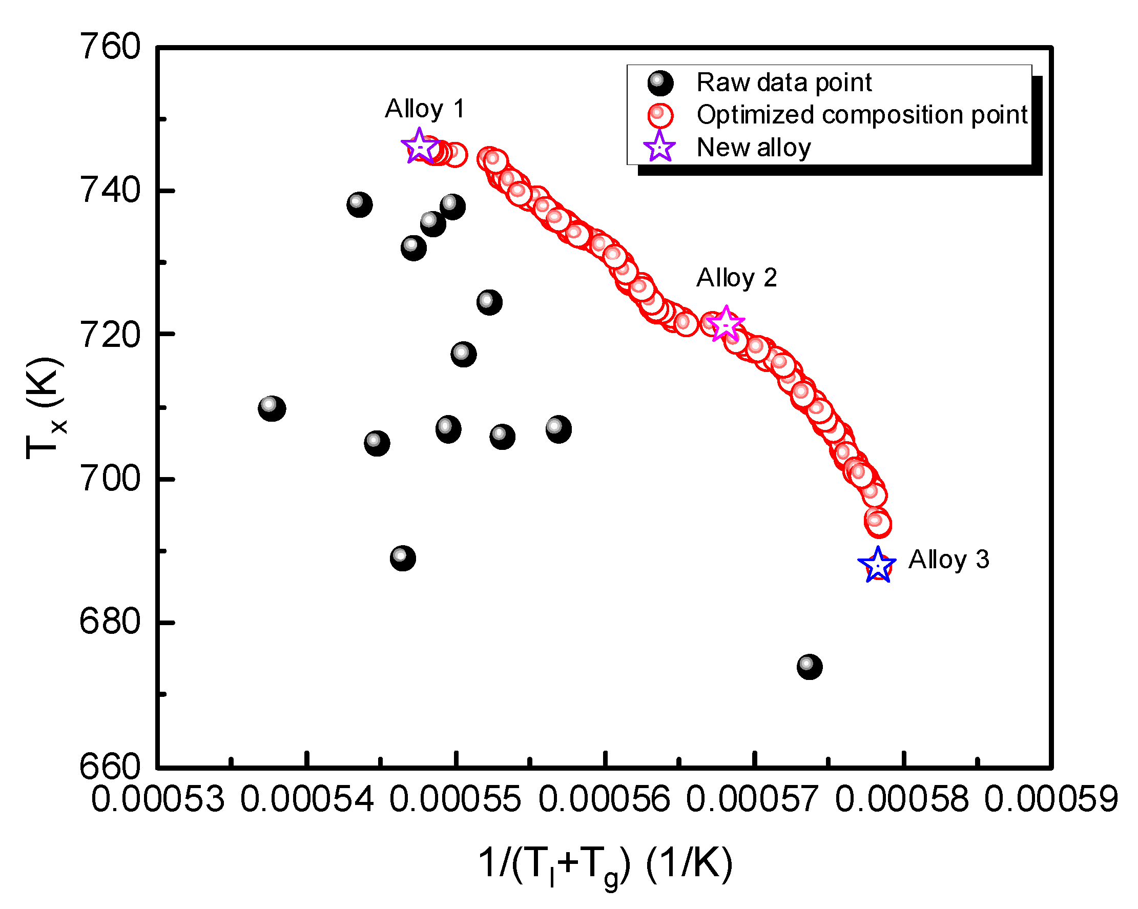
3.4. Composition Optimization Design

Based on the depicted figure, it is evident that there are shared key features for T_l, T_x, and T_g, and these features exert varying influences on the parameters. Taking the previously mentioned γ = T_x/(T_l + T_g) as an example, to optimize the GFA of MGs, it is essential to maximize γ. This, in turn, requires a compositional design approach that simultaneously maximizes T_x and 1/(T_l + T_g).

Taking the Zr-Cu-Ni-Al system as an example, the search range for each element is as follows: Cu: 5~20 wt.%, Ni: 5~20 wt.%, and Al: 5~10 wt.%. Each element is systematically varied within the compositional search space with a step size of 0.01 wt.%. The NSGA-II algorithm is utilized to simultaneously optimize T_x and (T_l + T_g) with the following specific parameter settings: the initial population size is 200, and the number of evolution generations is 300. It utilizes the polymutation mutation operator with a mutation rate of 0.02. The XOVR crossover operator is employed with a crossover rate of 0.9. The chromosomes are encoded using the RI encoding method. The primary objective is to identify a non-dominated set of compositions that maximize T_x and 1/(T_l + T_g), thereby facilitating the swift design of metallic glass compositions. Figure 11 visually presents the distribution of both the raw and optimized data for T_x and 1/(T_l + T_g) within the Zr-Cu-Ni-Al system. The optimized data’s Pareto front shifted towards the upper right corner compared to that of the raw data. This shift signifies that the application of a non-dominated genetic algorithm yielded superior composition designs. Three representative composition points are identified as Alloy 1: Zr61.46Cu8.96Ni19.98Al9.60, Alloy 2: Zr68.43Cu15.68Ni10.40Al5.49, and Alloy 3: Zr62.81Cu15.01Ni13.45Al8.73.

The rapid design of alloys with high GFA is realized by machine learning, which effectively saves time and resources. However, the designed alloys need to be verified by experiments to prove the accuracy of the prediction model.

4. Conclusions

(1)

By developing a discriminative model based on alloy composition, the XGC model exhibits superior performance compared to the other three commonly employed classification models. With an impressive classification accuracy of 98%, it effectively determines GFA.

(2)

In the context of alloys capable of forming metallic glasses, the ETR algorithm is utilized to establish predictive models for T_l, T_x, and T_g. The R² values associated with these models all exceed 0.91, thereby demonstrating their exceptional predictive accuracy.

(3)

To enhance the simplicity of the models, various feature selection techniques, including variance, correlation, embedding, recursive, and exhaustive methods, are employed. These techniques enable the identification of crucial features for T_l, T_x, and T_g. While ensuring the preservation of model accuracy, the dimensionality of the features is effectively reduced, resulting in the final selection of four key features for each property.

(4)

The interpretability analysis of the predictive models for T_l, T_x, and T_g is performed by employing feature importance, PDP, and ICE. Through this comprehensive analysis, the influence patterns of each key feature on the target variables are uncovered, offering valuable insights for future alloy design. These findings serve as crucial reference directions for subsequent endeavors in alloy design.

(5)

In the case of the Zr-Cu-Al-Ni system, the GFA of MGs is evaluated through the parameter γ(T_x/(T_l + T_g)). The primary goal is to maximize γ by extensively exploring the compositional space of the Zr-Cu-Al-Ni system using a genetic algorithm. This innovative approach is aimed at enhancing the efficiency of MG development.

References

1. Egami, T.; Iwashita, T.; Dmowski, W. Mechanical Properties of Metallic Glasses. Metals 2013, 3, 77–113. [Google Scholar] [CrossRef]
2. Xu, D.; Lohwongwatana, B.; Duan, G.; Johnson, W.L.; Garland, C. Bulk metallic glass formation in binary Cu-rich alloy series—Cu100−xZrx (x = 34, 36, 38.2, 40 at.%) and mechanical properties of bulk Cu64Zr36 glass. Acta Mater. 2004, 52, 2621–2624. [Google Scholar] [CrossRef]
3. Wang, W.H. The elastic properties, elastic models and elastic perspectives of metallic glasses. Prog. Mater. Sci. 2012, 57, 487–656. [Google Scholar] [CrossRef]
4. Peter, W.H.; Buchanan, R.A.; Liu, C.T.; Liaw, P.K.; Morrison, M.L.; Horton, J.A.; Carmichael, C.A.; Wright, J.L. Localized corrosion behavior of a zirconium-based bulk metallic glass relative to its crystalline state. Intermetallics 2002, 10, 1157–1162. [Google Scholar] [CrossRef]
5. Jiao, Z.B.; Li, H.X.; Gao, J.E.; Wu, Y.; Lu, Z.P. Effects of alloying elements on glass formation, mechanical and soft-magnetic properties of Fe-based metallic glasses. Intermetallics 2011, 19, 1502–1508. [Google Scholar] [CrossRef]
6. Reddy, G.J.; Kandavalli, M.; Saboo, T.; Rao, A.K.P. Prediction of Glass Forming Ability of Bulk Metallic Glasses Using Machine Learning. Integr. Mater. Manuf. Innov. 2021, 10, 610–626. [Google Scholar] [CrossRef]
7. Xu, M.; Wang, J.; Sun, Y.; Zhu, S.; Zhang, T.; Guan, S. Prediction of glass-forming ability in ternary alloys based on machine learning method. J. Non-Cryst. Solids 2023, 616, 122476. [Google Scholar] [CrossRef]
8. Majid, A.; Ahsan, S.B.; Tariq, N.u.H. Modeling glass-forming ability of bulk metallic glasses using computational intelligent techniques. Appl. Soft Comput. 2015, 28, 569–578. [Google Scholar] [CrossRef]
9. Peng, L.; Long, Z.; Zhao, M. Determination of glass forming ability of bulk metallic glasses based on machine learning. Comput. Mater. Sci. 2021, 195, 110480. [Google Scholar] [CrossRef]
10. Xiong, J.; Shi, S.; Zhang, T. A machine-learning approach to predicting and understanding the properties of amorphous metallic alloys. Mater. Des. 2020, 187, 108378. [Google Scholar] [CrossRef]
11. Long, Z.; Liu, W.; Zhong, M.; Zhang, Y.; Zhao, M.; Liao, G.; Chen, Z. A new correlation between the characteristics temperature and glass-forming ability for bulk metallic glasses. J. Therm. Anal. Calorim. 2018, 132, 1645–1660. [Google Scholar] [CrossRef]
12. Mastropietro, D.G.; Moya, J.A. Design of Fe-based bulk metallic glasses for maximum amorphous diameter (Dmax) using machine learning models. Comput. Mater. Sci. 2021, 188, 110230. [Google Scholar] [CrossRef]
13. Lu, F.; Liang, Y.; Wang, X.; Gao, T.; Chen, Q.; Liu, Y.; Zhou, Y.; Yuan, Y.; Liu, Y. Prediction of amorphous forming ability based on artificial neural network and convolutional neural network. Comput. Mater. Sci. 2022, 210, 111464. [Google Scholar] [CrossRef]
14. Turnbull, D. Under what conditions can a glass be formed? Contemp. Phys. 1969, 10, 473–488. [Google Scholar] [CrossRef]
15. Chen, H.S. Thermodynamic considerations on the formation and stability of metallic glasses. Scr. Metall. 1974, 22, 1505–1511. [Google Scholar]
16. Inoue, A. Stabilization of metallic supercooled liquid and bulk amorphous alloys. Acta Mater. 2000, 48, 279–306. [Google Scholar] [CrossRef]
17. Lu, Z.P.; Liu, C.T. A new glass-forming ability criterion for bulk metallic glasses. Acta Mater. 2002, 50, 3501–3512. [Google Scholar] [CrossRef]
18. Ward, L.; O’Keeffe, S.C.; Stevick, J.; Jelbert, G.R.; Aykol, M.; Wolverton, C. A machine learning approach for engineering bulk metallic glass alloys. Acta Mater. 2018, 159, 102–111. [Google Scholar] [CrossRef]
19. Yu, J.Z. Nonequilibrium Phase Diagrams of Ternary Amorphous Alloys; Springer: Berlin/Heidelberg, Germany, 1997. [Google Scholar]
20. Huang, X.; Chang, C.; Chang, Z.; Wang, X.; Cao, Q.; Shen, B.; Inoue, A.; Jiang, J. Formation of bulk metallic glasses in the Fe–M–Y–B (M = transition metal) system. J. Alloys Compd. 2008, 460, 708–713. [Google Scholar] [CrossRef]
21. Kato, H.; Chen, H.S.; Inoue, A. Relationship between thermal expansion coefficient and glass transition temperature in metallic glasses. Scr. Mater. 2008, 58, 1106–1109. [Google Scholar] [CrossRef]
22. An, W.; Cai, A.; Li, J.; Luo, Y.; Li, T.; Xiong, X.; Liu, Y.; Pan, Y. Glass formation and non-isothermal crystallization of Zr62.5Al12.1Cu7.95Ni17.45 bulk metallic glass. J. Non-Cryst. Solids 2009, 355, 1703–1706. [Google Scholar] [CrossRef]
23. González, S.; Figueroa, I.; Todd, I. Influence of minor alloying additions on the glass-forming ability of Mg–Ni–La bulk metallic glasses. J. Alloys Compd. 2009, 484, 612–618. [Google Scholar] [CrossRef]
24. Long, Z.; Wei, H.; Ding, Y.; Zhang, P.; Xie, G.; Inoue, A. A new criterion for predicting the glass-forming ability of bulk metallic glasses. J. Alloys Compd. 2009, 475, 207–219. [Google Scholar] [CrossRef]
25. Huang, X.; Chang, C.; Chang, Z.; Inoue, A.; Jiang, J. Glass forming ability, mechanical and magnetic properties in Fe–W–Y–B alloys. Mater. Sci. Eng. A 2010, 527, 1952–1956. [Google Scholar] [CrossRef]
26. Guo, S.-f.; Ye, S. Design of high strength Fe-(P, C)-based bulk metallic glasses with Nb addition. Trans. Nonferrous Met. Soc. China 2011, 21, 2433–2437. [Google Scholar] [CrossRef]
27. Hua, N.; Li, R.; Wang, H.; Wang, J.; Li, Y.; Zhang, T. Formation and mechanical properties of Ni-free Zr-based bulk metallic glasses. J. Alloys Compd. 2011, 509, S175–S178. [Google Scholar] [CrossRef]
28. Kucuk, I.; Aykol, M.; Uzun, O.; Yildirim, M.; Kabaer, M.; Duman, N.; Yilmaz, F.; Erturk, K.; Akdeniz, M.V.; Mekhrabov, A.O. Effect of (Mo, W) substitution for Nb on glass forming ability and magnetic properties of Fe–Co-based bulk amorphous alloys fabricated by centrifugal casting. J. Alloys Compd. 2011, 509, 2334–2337. [Google Scholar] [CrossRef]
29. Sheng, G.; Liu, C.T. Phase stability in high entropy alloys: Formation of solid-solution phase or amorphous phase. Prog. Nat. Sci. Mater. Int. 2011, 21, 433–446. [Google Scholar]
30. Samavatian, M.; Gholamipour, R.; Samavatian, V. Discovery of novel quaternary bulk metallic glasses using a developed correlation-based neural network approach. Comput. Mater. Sci. 2021, 186, 110025. [Google Scholar] [CrossRef]
31. Deshmukh, A.A.; Khond, A.A.; Bhatt, J.G.; Palikundwar, U.A. Understanding the role of Er on glass forming ability parameters and critical cooling rate in Fe–based multicomponent bulk metallic glasses. J. Alloys Compd. 2020, 819, 152938. [Google Scholar] [CrossRef]
32. Li, B.; Sun, W.C.; Qi, H.N.; Lv, J.W.; Wang, F.L.; Ma, M.Z.; Zhang, X.Y. Effects of Ag substitution for Fe on glass-forming ability, crystallization kinetics, and mechanical properties of Ni-free Zr-Cu-Al-Fe bulk metallic glasses. J. Alloys Compd. 2020, 827, 154385. [Google Scholar] [CrossRef]
33. Jia, H.; Xie, X.; Zhao, L.; Wang, J.; Gao, Y.; Dahmen, K.A.; Li, W.; Liaw, P.K.; Ma, C. Effects of similar-element-substitution on the glass-forming ability and mechanical behaviors of Ti-Cu-Zr-Pd bulk metallic glasses. J. Mater. Res. Technol. 2018, 7, 261–269. [Google Scholar] [CrossRef]
34. Hu, F.; Yuan, C.; Luo, Q.; Yang, W.; Shen, B. Effects of heavy rare-earth addition on glass-forming ability, thermal, magnetic, and mechanical properties of Fe-RE-B-Nb (RE = Dy, Ho, Er or Tm) bulk metallic glass. J. Non-Cryst. Solids 2019, 525, 119681. [Google Scholar] [CrossRef]
35. Hu, F.; Luo, Q.; Shen, B. Thermal, magnetic and magnetocaloric properties of FeErNbB metallic glasses with high glass-forming ability. J. Non-Cryst. Solids 2019, 512, 184–188. [Google Scholar] [CrossRef]
36. Hasani, S.; Rezaei-Shahreza, P.; Seifoddini, A.; Hakimi, M. Enhanced glass forming ability, mechanical, and magnetic properties of Fe41Co7Cr15Mo14Y2C15B6 bulk metallic glass with minor addition of Cu. J. Non-Cryst. Solids 2018, 497, 40–44. [Google Scholar] [CrossRef]
37. Gu, J.-L.; Shao, Y.; Yao, K.-F. The novel Ti-based metallic glass with excellent glass forming ability and an elastic constant dependent glass forming criterion. Materialia 2019, 8, 100433. [Google Scholar] [CrossRef]
38. Ge, J.; He, H.; Zhou, J.; Lu, C.; Dong, W.; Liu, S.; Lan, S.; Wu, Z.; Wang, A.; Wang, L.; et al. In-situ scattering study of a liquid-liquid phase transition in Fe-B-Nb-Y supercooled liquids and its correlation with glass-forming ability. J. Alloys Compd. 2019, 787, 831–839. [Google Scholar] [CrossRef]
39. Zhu, J.; Wang, C.; Han, J.; Yang, S.; Xie, G.; Jiang, H.; Chen, Y.; Liu, X. Formation of Zr-based bulk metallic glass with large amount of yttrium addition. Intermetallics 2018, 92, 55–61. [Google Scholar] [CrossRef]
40. Yang, G.; Lian, J.; Wang, R.; Wu, N. Similar atom substitution effect on the glass forming ability in (La Ce) Al-(Ni Co) bulk metallic glasses using electron structure guiding. J. Alloys Compd. 2019, 786, 250–256. [Google Scholar] [CrossRef]
41. Yang, Y.J.; Cheng, B.Y.; Lv, J.W.; Li, B.; Ma, M.Z.; Zhang, X.Y.; Li, G.; Liu, R.P. Effect of Ag substitution for Ti on glass-forming ability, thermal stability and mechanical properties of Zr-based bulk metallic glasses. Mater. Sci. Eng. A 2019, 746, 229–238. [Google Scholar] [CrossRef]
42. Wada, T.; Jiang, J.; Yubuta, K.; Kato, H.; Takeuchi, A. Septenary Zr–Hf–Ti–Al–Co–Ni–Cu high-entropy bulk metallic glasses with centimeter-scale glass-forming ability. Materialia 2019, 7, 100372. [Google Scholar] [CrossRef]
43. Dong, Q.; Pan, Y.J.; Tan, J.; Qin, X.M.; Li, C.J.; Gao, P.; Feng, Z.X.; Calin, M.; Eckert, J. A comparative study of glass-forming ability, crystallization kinetics and mechanical properties of Zr55Co25Al20 and Zr52Co25Al23 bulk metallic glasses. J. Alloys Compd. 2019, 785, 422–428. [Google Scholar] [CrossRef]
44. Xue, L.; Li, J.; Yang, W.; Yuan, C.; Shen, B. Effect of Fe substitution on magnetocaloric effects and glass-forming ability in Gd-based metallic glasses. Intermetallics 2018, 93, 67–71. [Google Scholar] [CrossRef]
45. Cao, D.; Wu, Y.; Liu, X.J.; Wang, H.; Wang, X.Z.; Lu, Z.P. Enhancement of glass-forming ability and plasticity via alloying the elements having positive heat of mixing with Cu in Cu48Zr48Al4 bulk metallic glass. J. Alloys Compd. 2019, 777, 382–391. [Google Scholar] [CrossRef]
46. Malekan, M.; Rashidi, R.; Shabestari, S.G. Mechanical properties and crystallization kinetics of Er-containing Cu-Zr-Al bulk metallic glasses with excellent glass forming ability. Vacuum 2020, 174, 109223. [Google Scholar] [CrossRef]
47. Saini, S.; Srivastava, A.P.; Neogy, S. The effect of Ag addition on the crystallization kinetics and glass forming ability of Zr-(CuAg)-Al bulk metallic glass. J. Alloys Compd. 2019, 772, 961–967. [Google Scholar] [CrossRef]
48. Liang, D.-d.; Wei, X.; Chang, C.; Li, J.; Wang, X.; Shen, J. Effect of W addition on the glass forming ability and mechanical properties of Fe-based metallic glass. J. Alloys Compd. 2018, 731, 1146–1150. [Google Scholar] [CrossRef]
49. Rahvard, M.M.; Tamizifar, M.; Boutorabi, S.M.A. Zr-Co(Cu)-Al bulk metallic glasses with optimal glass-forming ability and their compressive properties. Trans. Nonferrous Met. Soc. China 2018, 28, 1543–1552. [Google Scholar] [CrossRef]
50. Zhang, T.; Long, Z.; Peng, L.; Li, Z. Prediction of glass forming ability of bulk metallic glasses based on convolutional neural network. J. Non-Cryst. Solids 2022, 595, 121846. [Google Scholar] [CrossRef]
51. Ma, S.; Ran, Y.; Liang, X.; Jiang, L.; Li, Y.; Wang, X.; Yao, M.; Zhang, W. Unveiling the role of Y content in glass-forming ability and soft magnetic properties of Co-Y-B metallic glasses by experiment and ab initio molecular dynamics simulations. J. Alloys Compd. 2022, 902, 163637. [Google Scholar] [CrossRef]
52. Malekan, M.; Rashidi, R.; Shabestari, S.G.; Eckert, J. Thermodynamic and kinetic interpretation of the glass-forming ability of Y-containing Cu-Zr-Al bulk metallic glasses. J. Non-Cryst. Solids 2022, 576, 121266. [Google Scholar] [CrossRef]
53. Wen, S.; Dai, C.; Mao, W.; Zhao, Y.; Han, G.; Wang, X. Effects of Ag and Co microalloying on glass-forming abilities and plasticity of Cu-Zr-Al based bulk metallic glasses. Mater. Des. 2022, 220, 110896. [Google Scholar] [CrossRef]
54. Ren, J.; Li, Y.; Liang, X.; Kato, H.; Zhang, W. Role of Fe substitution for Co on thermal stability and glass-forming ability of soft magnetic Co-based Co-Fe-B-P-C metallic glasses. Intermetallics 2022, 147, 107598. [Google Scholar] [CrossRef]
55. Ma, S.; Zhang, J.; Wang, X.; Umetsu, R.Y.; Jiang, L.; Zhang, W.; Yao, M. Structural Origins for Enhanced Thermal Stability and Glass-Forming Ability of Co–B Metallic Glasses with Y and Nb Addition. Acta Metall. Sin. (Engl. Lett.) 2023, 36, 962–972. [Google Scholar] [CrossRef]
56. Zhu, J.; Gao, W.; Cheng, S.; Liu, X.; Yang, X.; Tian, J.; Ma, J.; Shen, J. Improving the glass forming ability and plasticity of ZrCuNiAlTi metallic glass by substituting Zr with Sc. J. Alloys Compd. 2022, 909, 164679. [Google Scholar] [CrossRef]
57. Ohashi, Y.; Wada, T.; Kato, H. High-entropy design and its influence on glass-forming ability in Zr–Cu-based metallic glass. J. Alloys Compd. 2022, 915, 165366. [Google Scholar] [CrossRef]
58. Liu, X.W.; Long, Z.L.; Zhang, W.; Yang, L.M. Key feature space for predicting the glass-forming ability of amorphous alloys revealed by gradient boosted decision trees model. J. Alloys Compd. 2022, 901, 163606. [Google Scholar] [CrossRef]
59. Wang, Y.; Wang, A.; Li, H.; Zhang, H.; Zhu, Z. The effect of minor alloying on the glass forming ability and crystallization reaction of Ti32.8Zr30.2Cu9M5.3Be22.7 (M = Fe, Co, and Ni) bulk metallic glass. J. Mater. Res. Technol. 2022, 18, 3035–3043. [Google Scholar] [CrossRef]
60. Zhang, S.; Wei, C.; Shi, Z.; Zhang, H.; Ma, M. Effect of Fe addition on the glass-forming ability, stability, and mechanical properties of Zr50Cu34-Fe Al8Ag8 metallic glasses. J. Alloys Compd. 2022, 929, 167334. [Google Scholar] [CrossRef]
61. Zhou, Y.; Zhao, L.; Qu, Y.; Hu, L.; Qi, L.; Qu, F.; He, S.; Liu, X. Effect of Yttrium Doping on Glass-Forming Ability, Thermal Stability, and Corrosion Resistance of Zr50.7Cu28Ni9Al12.3 Bulk Metallic Glass. Metals 2023, 13, 521. [Google Scholar] [CrossRef]
62. Ma, X.; Li, Q.; Xie, L.; Chang, C.; Li, H. Effect of Ni addition on the properties of CoMoPB bulk metallic glasses. J. Non-Cryst. Solids 2022, 587, 121573. [Google Scholar] [CrossRef]
63. Lu, S.; Li, X.; Liang, X.; He, J.; Shao, W.; Li, K.; Chen, J. Effect of Ho Addition on the Glass-Forming Ability and Crystallization Behaviors of Zr54Cu29Al10Ni7 Bulk Metallic Glass. Metals 2022, 15, 2516. [Google Scholar] [CrossRef] [PubMed]
64. Huang, Z.; Tao, P.; Long, Z.; Xiong, Z.; Zhu, X.; Xu, X.; Huang, Z.; Deng, H.; Lin, H.; Li, W.; et al. Effect of Ti addition on mechanical properties of Zr-based bulk metallic glasses. J. Non-Cryst. Solids 2023, 601, 122075. [Google Scholar] [CrossRef]
65. Peng, J.; Tang, B.; Wang, Q.; Bai, C.; Wu, Y.; Chen, Q.; Li, D.; Ding, D.; Xia, L.; Guo, X.; et al. Effect of heavy rare-earth (Dy, Tb, Gd) addition on the glass-forming ability and magneto-caloric properties of Fe89Zr7B4 amorphous alloy. J. Alloys Compd. 2022, 925, 166707. [Google Scholar] [CrossRef]
66. Diao, Y.; Yan, L.; Gao, K. Improvement of the machine learning-based corrosion rate prediction model through the optimization of input features. Mater. Des. 2021, 198, 109326. [Google Scholar] [CrossRef]
67. Lix, L.M.; Keselman, J.C.; Keselman, H.J. Consequences of Assumption Violations Revisited: A Quantitative Review of Alternatives to the One-Way Analysis of Variance F Test. Rev. Educ. Res. 1996, 66, 579–619. [Google Scholar]
68. Sekeh, S.Y.; Hero, A.O. Feature Selection For Mutlti-Labeled Variables Via Dependency Maximization. In Proceedings of the IEEE International Conference on Acoustics, Speech, Signal Processing, Brighton, UK, 12–17 May 2019; pp. 3127–3131. [Google Scholar]
69. Louw, N.; Steel, S.J. Variable selection in kernel Fisher discriminant analysis by means of recursive feature elimination. Comput. Stat. Data Anal. 2005, 51, 2043–2055. [Google Scholar] [CrossRef]
70. Wang, L.; Wang, Y.; Chang, Q. Feature Selection Methods for Big Data Bioinformatics: A Survey from the Search Perspective. Methods 2016, 111, 21–31. [Google Scholar] [CrossRef]
71. Islam, N.; Huang, W.; Zhuang, H.L. Machine learning for phase selection in multi-principal element alloys. Comput. Mater. Sci. 2018, 150, 230–235. [Google Scholar] [CrossRef]
72. Liu, Y.; Hou, T.; Yan, Z.; Yu, T.; Duan, J.; Xiao, Y.; Wu, K. The effect of element characteristics on bainite transformation start temperature using a machine learning approach. J. Mater. Sci. 2023, 58, 443–456. [Google Scholar] [CrossRef]
73. Meredig, B.; Agrawal, A.; Kirklin, S.; Saal, J.E.; Doak, J.W.; Thompson, A.; Zhang, K.; Choudhary, A.; Wolverton, C. Combinatorial screening for new materials in unconstrained composition space with machine learning. Phys. Rev. B 2014, 89, 094104. [Google Scholar] [CrossRef]
74. Friedman, J.H. Greedy Function Approximation: A Gradient Boosting Machine. Ann. Stat. 2001, 29, 1189–1232. [Google Scholar] [CrossRef]
75. Goldstein, A.; Kapelner, A.; Bleich, J.; Pitkin, E. Peeking Inside the Black Box: Visualizing Statistical Learning With Plots of Individual Conditional Expectation. J. Comput. Graph. Stat. 2015, 24, 44–65. [Google Scholar] [CrossRef]
76. Seibold, H.; Zeileis, A.; Hothorn, T. Model-Based Recursive Partitioning for Subgroup Analyses. Int. Stat. Rev. 2016, 12, 45–63. [Google Scholar] [CrossRef] [PubMed]
77. Yan, Z.; Li, L.; Cheng, L.; Chen, X.; Wu, K. New insight in predicting martensite start temperature in steels. J. Mater. Sci. 2022, 57, 11392–11410. [Google Scholar] [CrossRef]
78. Chand, S.; Wagner, M. Evolutionary many-objective optimization: A quick-start guide. Surv. Oper. Res. Manag. Sci. 2015, 20, 35–42. [Google Scholar] [CrossRef]
79. Liu, C.; Wang, X.; Cai, W.; Yang, J.; Su, H. Optimal Design of the Austenitic Stainless-Steel Composition Based on Machine Learning and Genetic Algorithm. Materials 2023, 16, 5633. [Google Scholar] [CrossRef]
80. Lu, Z.P.; Tan, H.; Ng, S.C.; Li, Y. The correlation between reduced glass transition temperature and glass forming ability of bulk metallic glasses. Scr. Mater. 2000, 42, 667–673. [Google Scholar] [CrossRef]
81. Chen, Q.; Shen, J.; Zhang, D.; Fan, H.; Sun, J.; McCartney, D.G. A new criterion for evaluating the glass-forming ability of bulk metallic glasses. Mater. Sci. Eng. A 2006, 433, 155–160. [Google Scholar] [CrossRef]
82. Yuan, Z.-Z.; Bao, S.-L.; Lu, Y.; Zhang, D.-P.; Yao, L. A new criterion for evaluating the glass-forming ability of bulk glass forming alloys. J. Alloys Compd. 2008, 459, 251–260. [Google Scholar] [CrossRef]
83. Ji, X.-l.; Pan, Y. A thermodynamic approach to assess glass-forming ability of bulk metallic glasses. Trans. Nonferrous Met. Soc. China 2009, 19, 1271–1279. [Google Scholar] [CrossRef]
84. Mondal, K.; Murty, B.S. On the parameters to assess the glass forming ability of liquids. J. Non-Cryst. Solids 2005, 351, 1366–1371. [Google Scholar] [CrossRef]
85. Du, X.H.; Huang, J.C.; Liu, C.T.; Lu, Z.P. New criterion of glass forming ability for bulk metallic glasses. J. Appl. Phys. 2007, 101, 086108. [Google Scholar] [CrossRef]
86. Błyskun, P.; Maj, P.; Kowalczyk, M.; Latuch, J.; Kulik, T. Relation of various GFA indicators to the critical diameter of Zr-based BMGs. J. Alloys Compd. 2015, 625, 13–17. [Google Scholar] [CrossRef]
87. Deng, R.; Long, Z.; Peng, L.; Kuang, D.; Ren, B. A new mathematical expression for the relation between characteristic temperature and glass-forming ability of metallic glasses. J. Non-Cryst. Solids 2020, 533, 119829. [Google Scholar] [CrossRef]
88. Guo, S.; Liu, C.T. New glass forming ability criterion derived from cooling consideration. Intermetallics 2010, 18, 2065–2068. [Google Scholar] [CrossRef]
89. Xiong, J.; Zhang, T.-Y.; Shi, S.-Q. Machine learning prediction of elastic properties and glass-forming ability of bulk metallic glasses. MRS Commun. 2019, 9, 576–585. [Google Scholar] [CrossRef]
90. Tripathi, M.K.; Ganguly, S.; Dey, P.; Chattopadhyay, P.P. Evolution of glass forming ability indicator by genetic programming. Comput. Mater. Sci. 2016, 118, 56–65. [Google Scholar] [CrossRef]
91. Long, T.; Long, Z.; Pang, B.; Li, Z.; Liu, X. Overcoming the challenge of the data imbalance for prediction of the glass forming ability in bulk metallic glasses. Mater. Today Commun. 2023, 35, 105610. [Google Scholar] [CrossRef]
92. Greer, A.L. Confusion by design. Nature 1993, 366, 303–304. [Google Scholar] [CrossRef]
93. Qiang, J.-B.; Wang, D.-H.; Bao, C.-M.; Wang, Y.-M.; Xu, W.-P.; Song, M.-L.; Dong, C. Formation rule for Al-based ternary quasi-crystals: Example of Al–Ni–Fe decagonal phase. J. Mater. Res. 2001, 16, 2653–2660. [Google Scholar] [CrossRef]
94. Wang, Y.M.; Qiang, J.B.; Wong, C.H.; Shek, C.H.; Dong, C. Composition rule of bulk metallic glasses and quasicrystals using electron concentration criterion. J. Mater. Res. 2003, 18, 642–648. [Google Scholar] [CrossRef]
95. Boer, F.R.d.; Mattens, W.C.M.; Boom, R.; Miedema, A.R.; Niessen, A.K. Cohesion in Metals. Transition Metal Alloys; North-Holland: Amsterdam, The Netherlands, 1988; Volume 1. [Google Scholar]
96. Miedema, A.R.; de Châtel, P.F.; de Boer, F.R. Cohesion in alloys—Fundamentals of a semi-empirical model. Physica B+C 1980, 100, 1–28. [Google Scholar] [CrossRef]
Figure 1. Process framework for establishing GFA prediction model based on machine learning.
Processes 11 02806 g001
Figure 2. Types of elements contained in datasets. * Lanthanides. ** Actinides.
Processes 11 02806 g002
Figure 3. Comparison of four classification models.
Processes 11 02806 g003
Figure 4. The performance of Tl, Tx, and Tg on different regression models of machine learning.
Processes 11 02806 g004
Figure 5. The comparison of predicted values and experimental values of Tl, Tx, and Tg by ETR model.
Processes 11 02806 g005
Figure 6. The feature screening process of Tl, Tx, and Tg.
Processes 11 02806 g006aProcesses 11 02806 g006b
Figure 7. The change of feature number in the process of feature screening.
Processes 11 02806 g007
Figure 8. Rank of feature importance corresponding to Tg, Tx, and Tl.
Processes 11 02806 g008
Figure 9. PDP plot analysis of key features on Tl. (a) Mean GSvolume_pa. (b) Mean Electronegativity. (c) Mean GSvolume_pa and Mean Electronegativity. (d) Mean Gsmagmon. (e) Avg_dev MendeleevNumb. (f) Mean Gsmagmon and Avg_dev MendeleevNumber.
Processes 11 02806 g009
Figure 10. ICE plot analysis of key features on Tl. (a) Mean GSvolume_pa (b) Mean Electronegativity (c) Mean Gsmagmon (d) Avg_dev MendeleevNumber.
Processes 11 02806 g010
Figure 11. Raw data and optimized data distribution of Zr-Cu-Ni-Al metallic glasses.
Processes 11 02806 g011