
Dynamic Modeling and Parameter Identification of Double Casing Joints for Aircraft Fuel Pipelines

Abstract
:1. Introduction
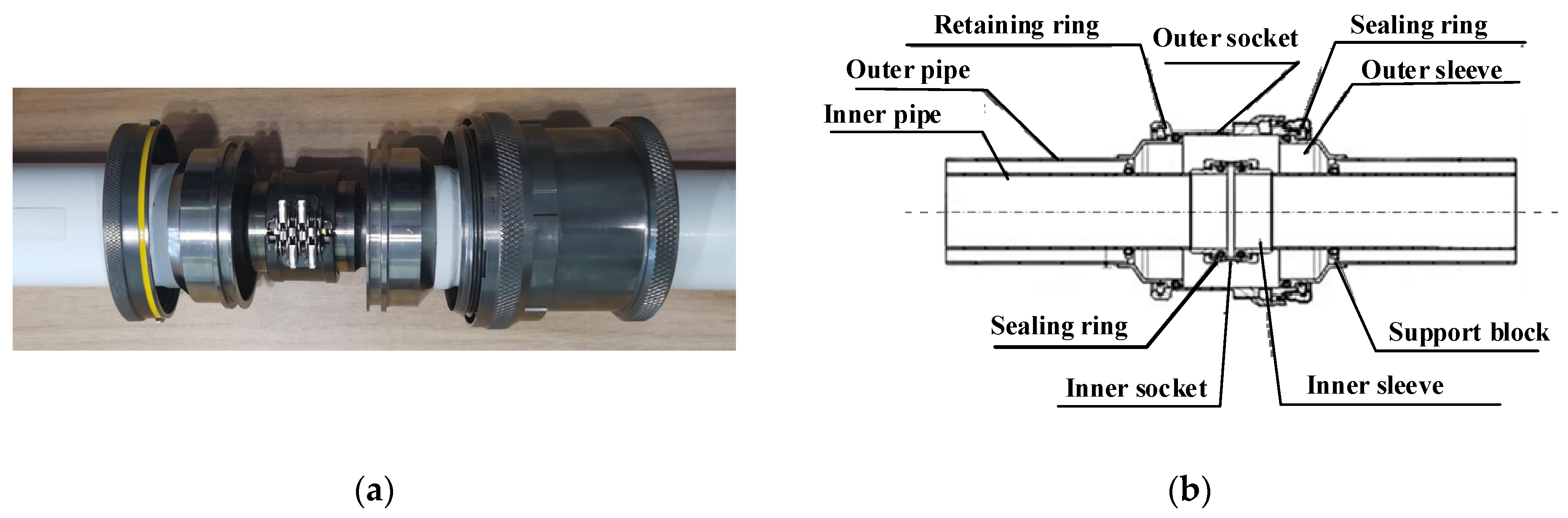
2. Working Principle
3. Theoretical Modeling
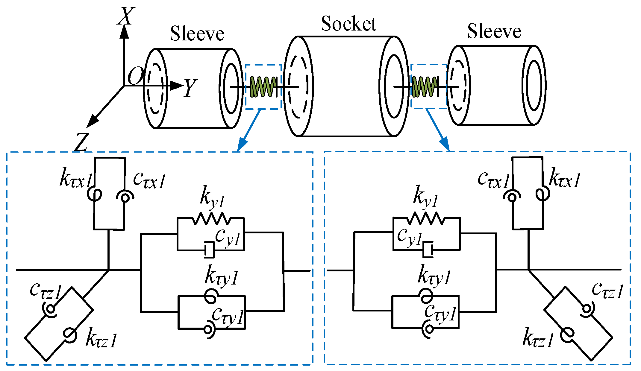
3.1. Force Analysis and Dynamic Modeling of Single-Layer Flexible Joints
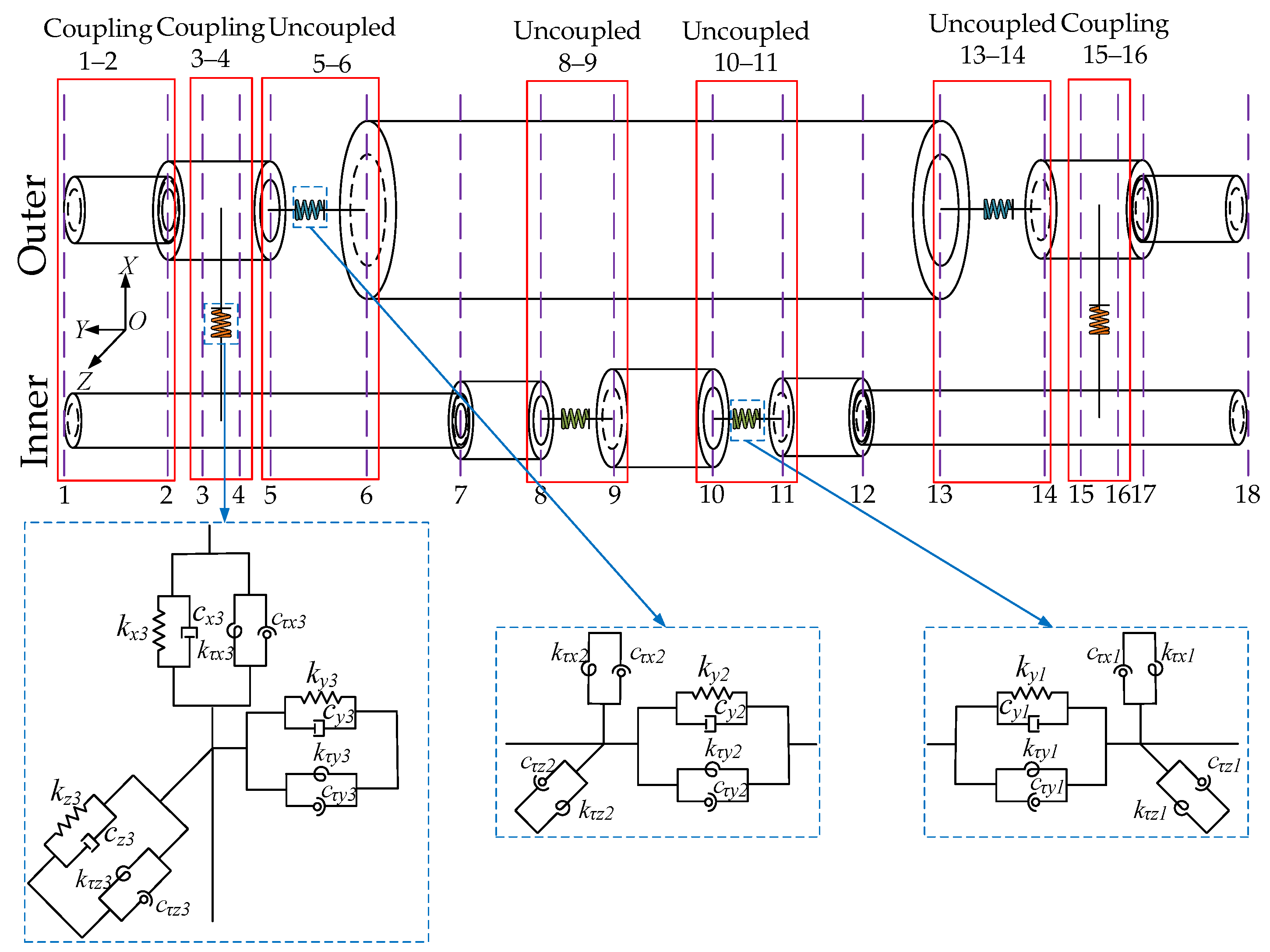
3.2. Dynamical Model of Double Casing Joint
4. Parameter Identification
4.1. Principle of FSM Method
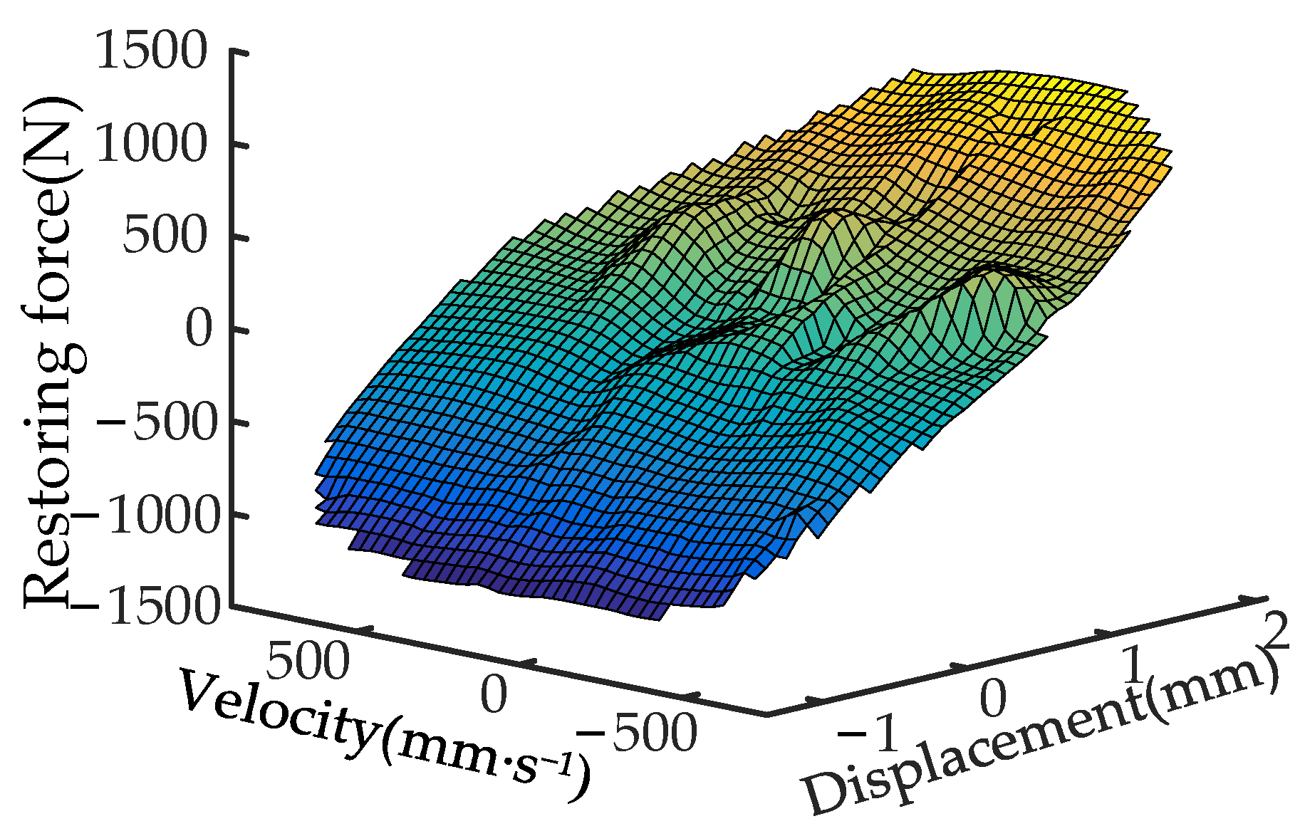
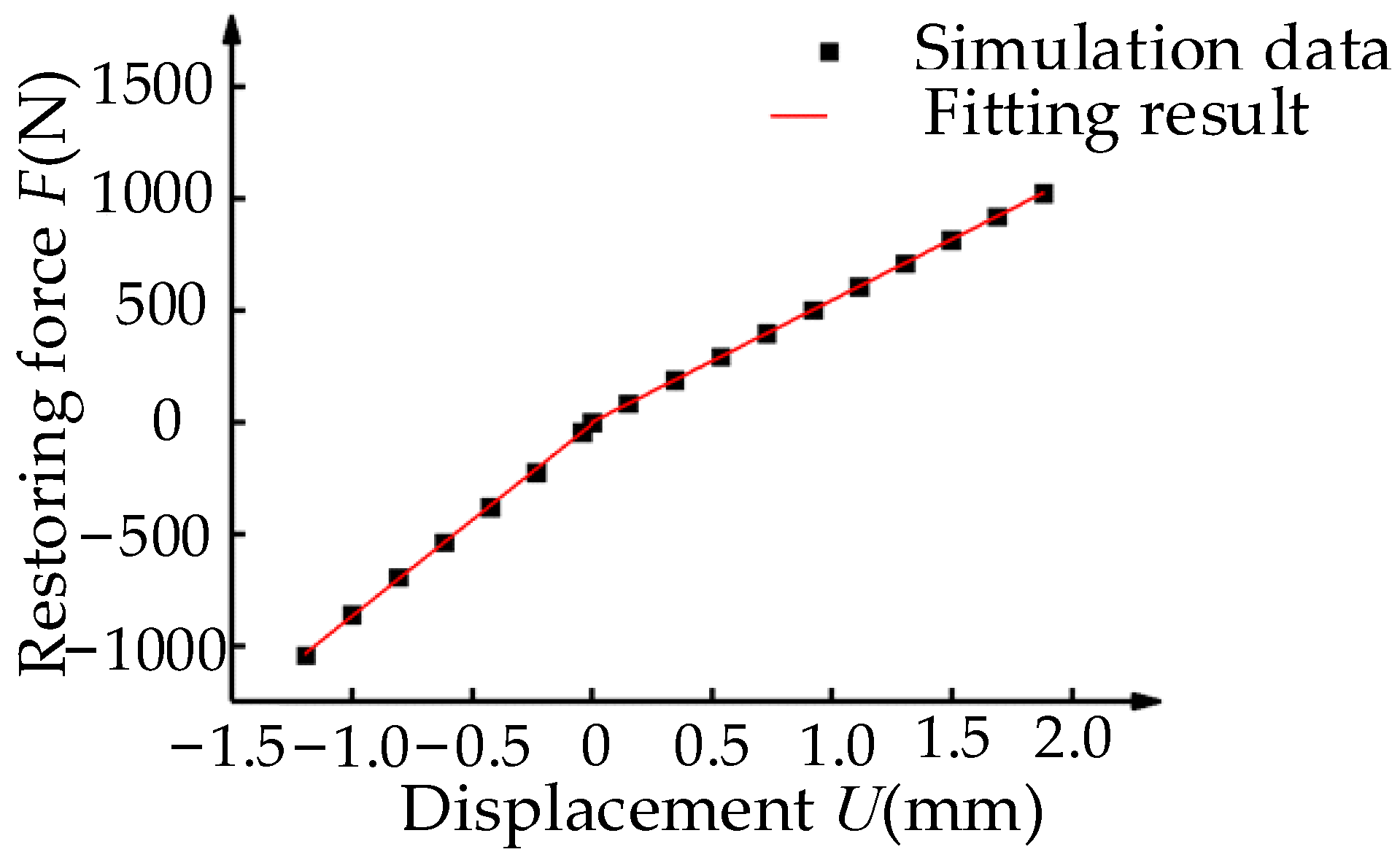
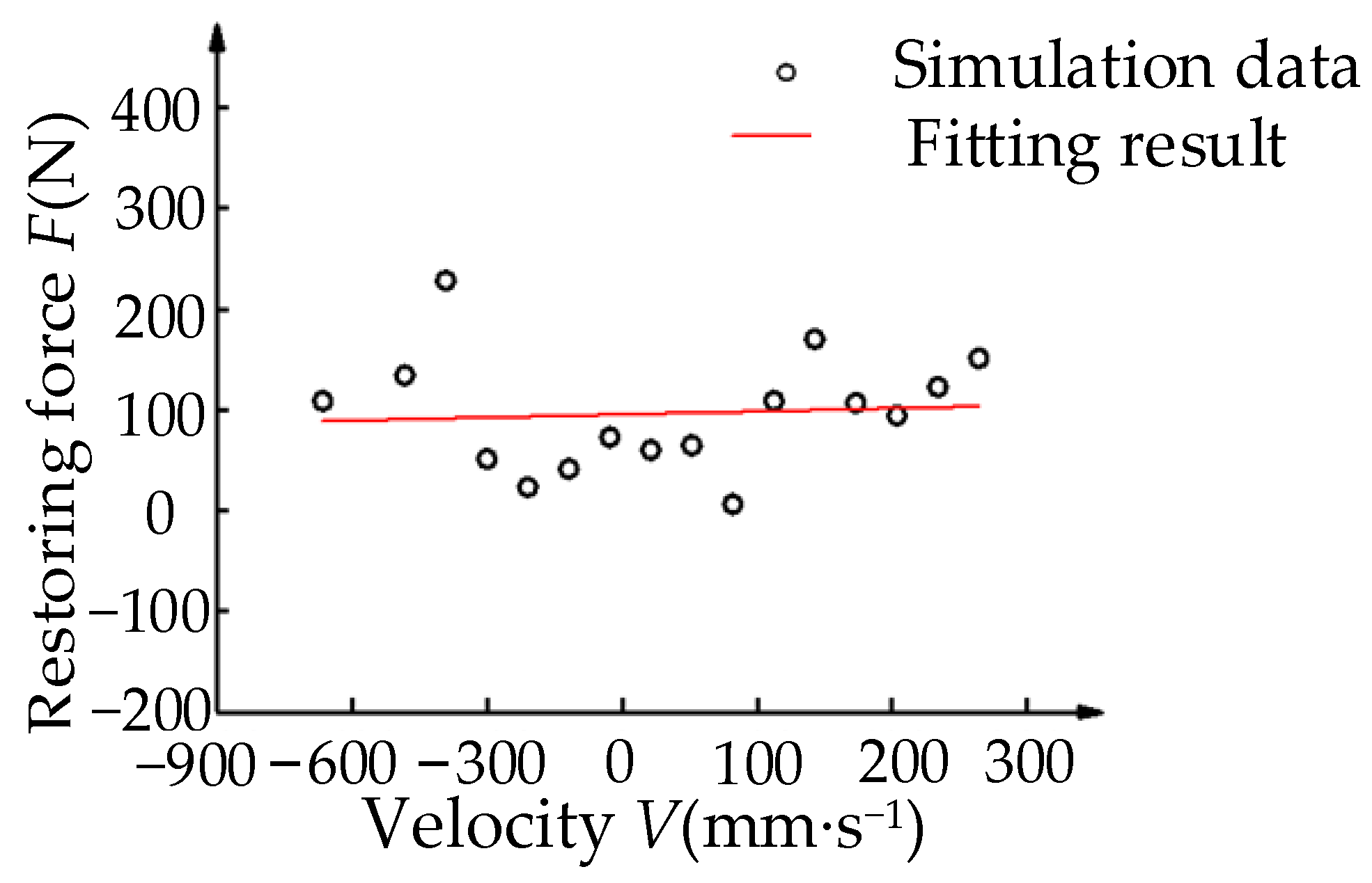
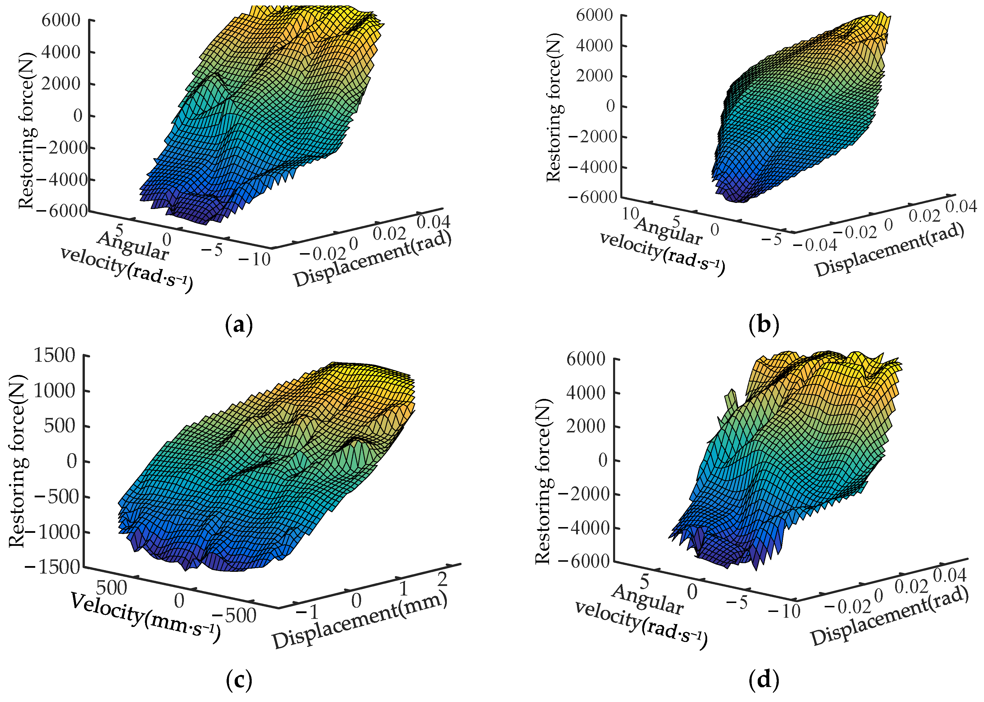
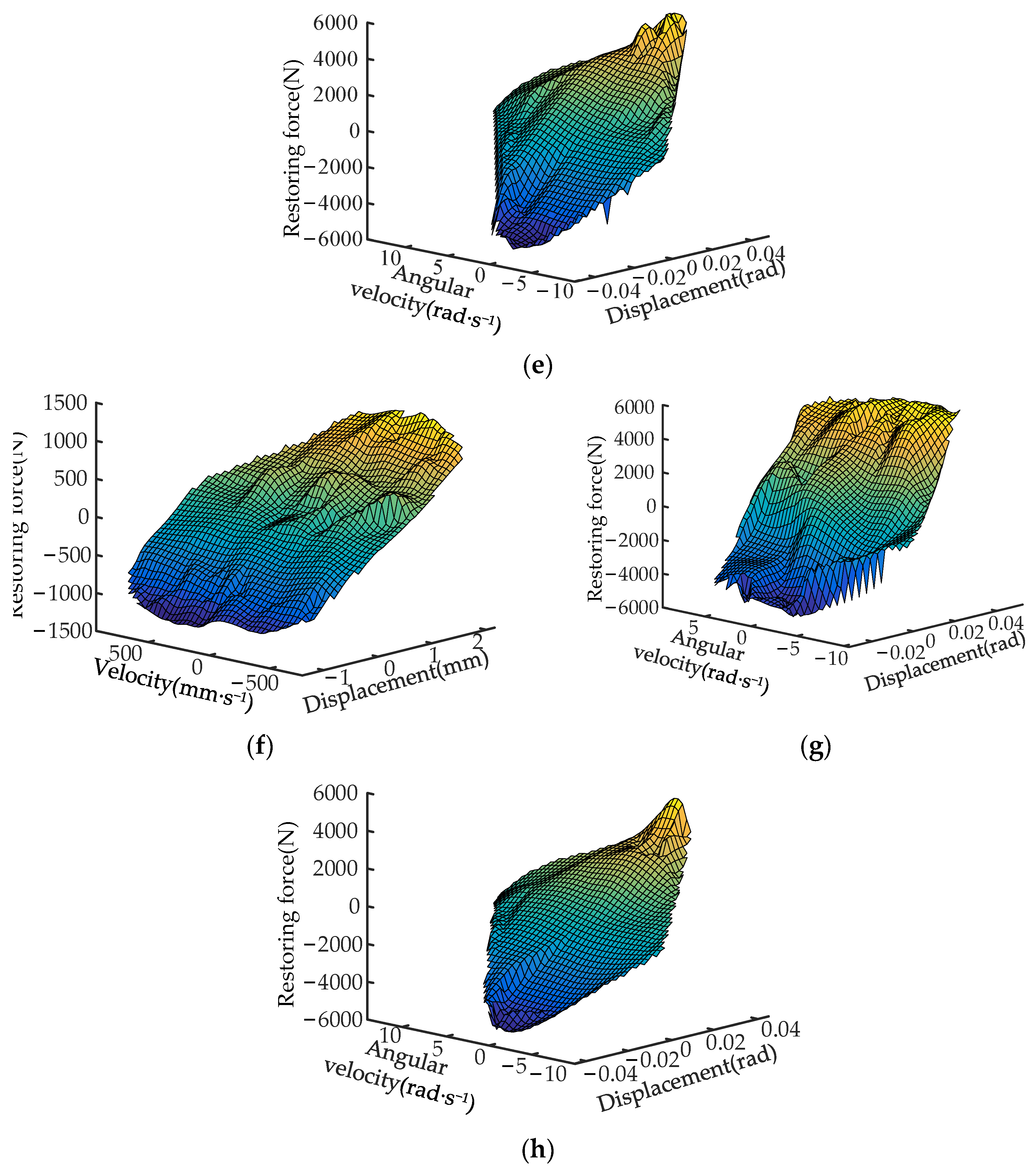
4.2. Parameter Identification Results of Joint
4.3. Parameter Identification Results of Support Block
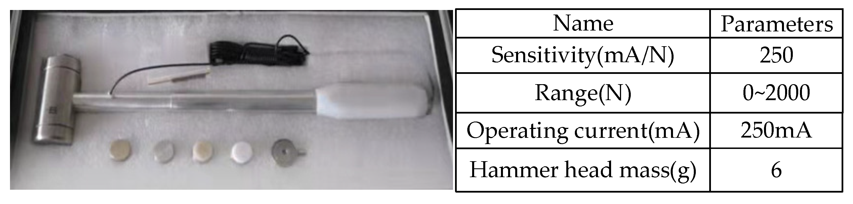
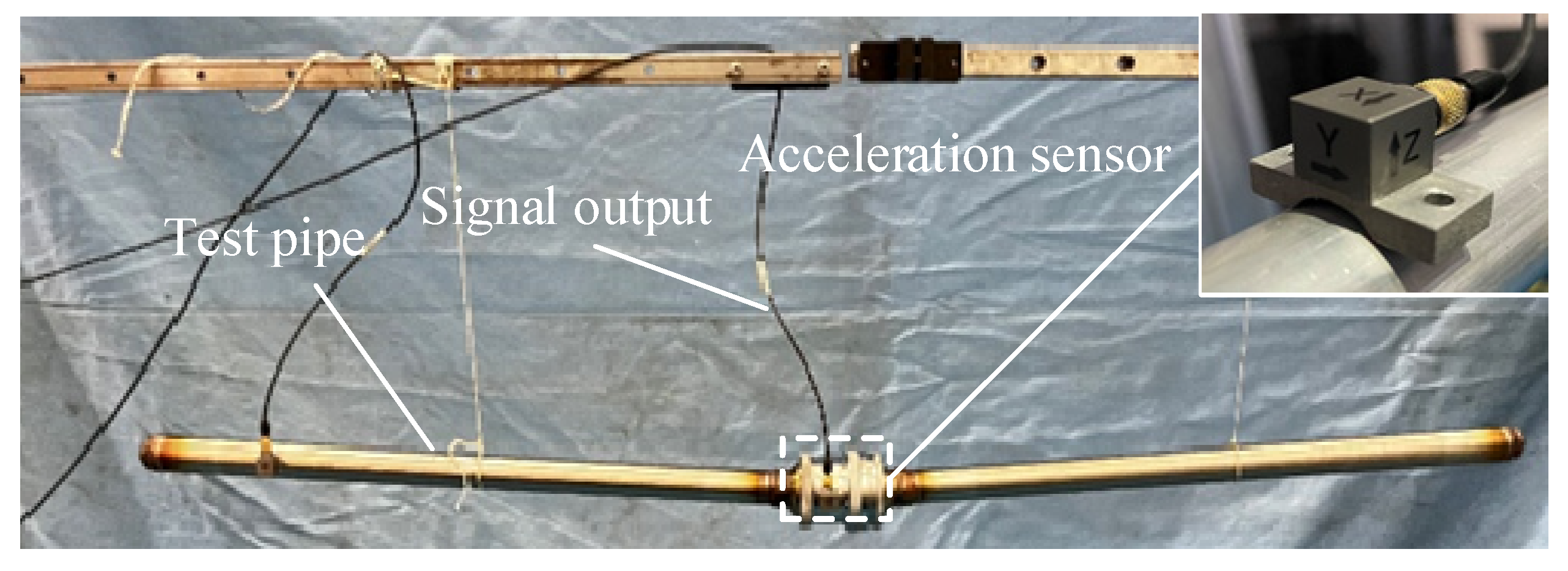
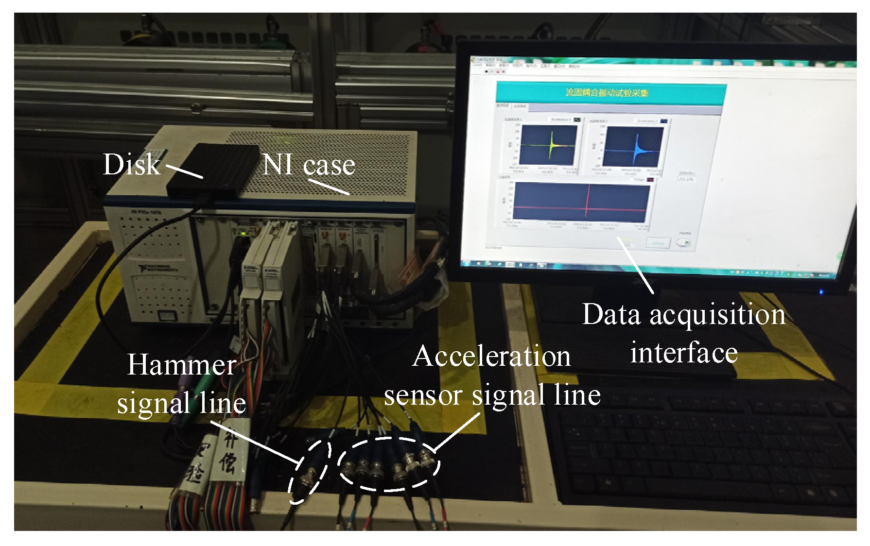
5. Free Modal Experiment
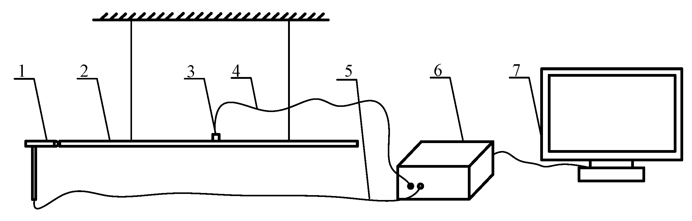
5.1. Experimental Method
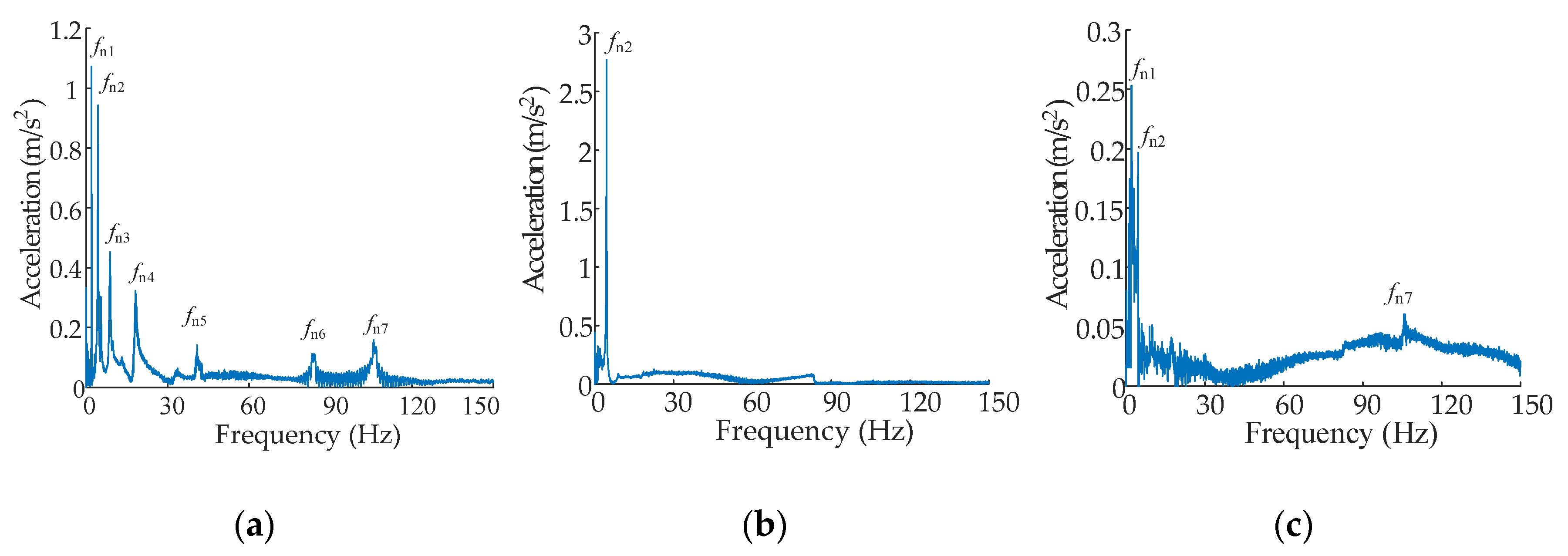
5.2. Experimental Result
6. Numerical Examples
7. Conclusions
Author Contributions
Funding
Data Availability Statement
Acknowledgments
Conflicts of Interest
Nomenclature
| V | Fluid velocity, m/s |
| P | Fluid pressure, MPa |
| Pipe velocity, m/s | |
| Forces in cross-section, N | |
| Moment, Nm | |
| x, y, z | Directional subscripts |
| Deflection angle of pipe, rad | |
| Angular velocity of pipe wall, rad/s | |
| m0 | Plug mass, kg |
References
- Wang, C.; Li, Y.G.; Yang, B.Y. Transient performance simulation of aircraft engine integrated with fuel and control systems. Appl. Therm. Eng. 2017, 114, 1029–1037. [Google Scholar] [CrossRef]
- Zhang, Z.; Li, B.; Yu, M.; Liu, Y.; Liu, W. Dynamic strength reliability analysis of an aircraft fuel pipe system. In Proceedings of the 2017 Second International Conference on Reliability Systems Engineering (ICRSE), Milan, Italy, 20–22 December 2017; IEEE: Piscataway, NJ, USA, 2017; pp. 1–6. [Google Scholar]
- Novichkov, V.M.; Filinov, N.I.; Kalinina, O.I. Assessment of the Technical Condition of the Aircraft Fuel System by Its Main Elements in Flight. In Proceedings of the 2020 International Multi-Conference on Industrial Engineering and Modern Technologies (FarEastCon), Vladivostok, Russia, 6–9 October 2020; IEEE: Piscataway, NJ, USA, 2020; pp. 1–4. [Google Scholar]
- Lamoureux, B.; Massé, J.R.; Mechbal, N. An approach to the health monitoring of a pumping unit in an aircraft engine fuel system. In PHM Society European Conference; PHM Society: Rochester, NY, USA, 2012. [Google Scholar]
- Wang, Y.; Ruan, C.; Lu, S.; Li, Z. A Study on the Movement Characteristics of Fuel in the Fuel Tank during the Maneuvering Process. Appl. Sci. 2023, 13, 8636. [Google Scholar] [CrossRef]
- Fredricson, H.; Johansen, T.; Klarbring, A.; Petersson, J. Topology optimization of frame structures with flexible joints. Struct. Multidiscip. Optim. 2003, 25, 199–214. [Google Scholar] [CrossRef]
- Melissianos, V.E.; Korakitis, G.P.; Gantes, C.J.; Bouckovalas, G.D. Numerical evaluation of the effectiveness of flexible joints in buried pipelines subjected to strike-slip fault rupture. Soil Dyn. Earthq. Eng. 2016, 90, 395–410. [Google Scholar] [CrossRef]
- Li, X.; Yao, Z.; Yang, M. A novel large thrust-weight ratio V-shaped linear ultrasonic motor with a flexible joint. Rev. Sci. Instrum. 2017, 88, 65003. [Google Scholar] [CrossRef]
- Ettefagh, M.H.; Naraghi, M.; Towhidkhah, F. Position Control of a Flexible Joint via Explicit Model Predictive Control: An Experimental Implementation. Emerg. Sci. J. 2019, 3, 146–156. [Google Scholar] [CrossRef]
- Hongbin, S.; Cai, W.; Zhuanli, Q.; Guocai, L. Numerical Research on Interfacial Damage and Sealing Reliability of Flexible Joint under Wide Temperature Range. J. Propuls. Technol. 2019, 40, 2313–2324. [Google Scholar]
- Song, C.; Du, Q.; Yang, S.; Feng, H.; Pang, H.; Li, C. Flexible joint parameters identification method based on improved tracking differentiator and adaptive differential evolution. Rev. Sci. Instrum. 2022, 93, 84706. [Google Scholar] [CrossRef]
- Xu, X.D.; Li, G.J.; Yuan, S. Application of Flexible Combine-Clamp in Digital Rapid Production for Aircraft Tube. Appl. Mech. Mater. 2013, 404, 777–781. [Google Scholar] [CrossRef]
- Melissianos, V.E.; Lignos, X.A.; Bachas, K.K.; Gantes, C.J. Experimental investigation of pipes with flexible joints under fault rupture. J. Constr. Steel Res. 2017, 128, 633–648. [Google Scholar] [CrossRef]
- Konstantinov, S.V.; Lalabekov, V.I.; Obolenskii, Y.G. Mathematical Model of the Gas-Hydraulic Control Actuator for the Swiveling Nozzle of the Solid Propellant Fuel Propulsion System with Flexible Joint. Russ. Aeronaut. 2019, 62, 222–228. [Google Scholar] [CrossRef]
- Ramezani, M.A.; Yousefi, S.; Fouladi, N. An experimental and numerical investigation of the effect of geometric parameters on the flexible joint nonlinear behavior for thrust vector control. Proc. Inst. Mech. Eng. Part G J. Aerosp. Eng. 2019, 233, 2772–2782. [Google Scholar] [CrossRef]
- Li, L.; Xu, W.; Tan, Y.; Yang, Y.; Yang, J.; Tan, D. Fluid-induced vibration evolution mechanism of multiphase free sink vortex and the multi-source vibration sensing method. Mech. Syst. Signal Process. 2023, 189, 110058. [Google Scholar] [CrossRef]
- Li, L.; Lu, B.; Xu, W.X.; Gu, Z.H.; Yang, Y.S.; Tan, D.P. Mechanism of multiphase coupling transport evolution of free sink vortex. Acta Phys. Sin. 2023, 72, 34702. [Google Scholar] [CrossRef]
- Zhang, X.M. Parametric studies of coupled vibration of cylindrical pipes conveying fluid with the wave propagation approach. Comput. Struct. 2002, 80, 287–295. [Google Scholar] [CrossRef]
- Xu, Y.; Johnston, D.N.; Jiao, Z.; Plummer, A.R. Frequency modelling and solution of fluid-structure interaction in complex pipelines. J. Sound Vib. 2014, 333, 2800–2822. [Google Scholar] [CrossRef]
- Selvarajan, S.; Tappe, A.A.; Heiduk, C.; Scholl, S.; Schenkendorf, R. Process Model Inversion in the Data-Driven Engineering Context for Improved Parameter Sensitivities. Processes 2022, 10, 1764. [Google Scholar] [CrossRef]
- Jin, H.; Liu, Z.; Zhang, H.; Liu, Y.; Zhao, J. A Dynamic Parameter Identification Method for Flexible Joints Based on Adaptive Control. IEEE/ASME Trans. Mechatron. 2018, 23, 2896–2908. [Google Scholar] [CrossRef]
- Asarin, E.; Donzé, A.; Maler, O.; Nickovic, D. Parametric Identification of Temporal Properties. In Proceedings of the Runtime Verification: Second International Conference, RV 2011, San Francisco, CA, USA, 27–30 September 2011; Springer: Berlin/Heidelberg, Germany, 2012; Volume 7186, pp. 147–160. [Google Scholar]
- Al-Hadid, M.A.; Wright, J.R. Estimation of mass and modal mass in the identification of non-linear single and multi degree of freedom systems using the force-state mapping approach. Mech. Syst. Signal Process. 1992, 6, 383–401. [Google Scholar] [CrossRef]
- Kimm, W.; Park, Y. Non-linear joint parameter identification by applying the force-state mapping technique in the frequency domain. Mech. Syst. Signal Process. 1994, 8, 519–529. [Google Scholar] [CrossRef]
- Wang, J.; Huang, H. Model and parameters identification of non-linear joint by force-state mapping in frequency domain. J. Mech. 2007, 23, 367–380. [Google Scholar] [CrossRef]
- Shu, Y.; Liu, Y.; Xu, Z.; Zhao, X.; Chen, M. Optimization of Hydraulic Fine Blanking Press Control System Based on System Identification. Processes 2023, 11, 59. [Google Scholar] [CrossRef]
- Gao, H.; Guo, C.; Quan, L.; Wang, S. Frequency Domain Analysis of Fluid–Structure Interaction in Aircraft Hydraulic Pipe with Complex Constraints. Processes 2022, 10, 1161. [Google Scholar] [CrossRef]
- Quan, L.; Luo, H.; Zhang, J. Harmonic Response Analysis of Axial Plunger Pump Shell Structure. Chin. Hydraul. Pneum. 2014, 5, 33–39. [Google Scholar]
- Chen, Y.; An, C.; Zhang, R.; Fu, Q.; Zhu, R. Research on Two-Way Contra-Rotating Axial-Flow Pump–Turbine with Various Blade Angles in Pump Mode. Processes 2023, 11, 1552. [Google Scholar] [CrossRef]
- Jalali, H.; Ahmadian, H.; Mottershead, J.E. Identification of nonlinear bolted lap-joint parameters by force-state mapping. Int. J. Solids Struct. 2007, 44, 8087–8105. [Google Scholar] [CrossRef]


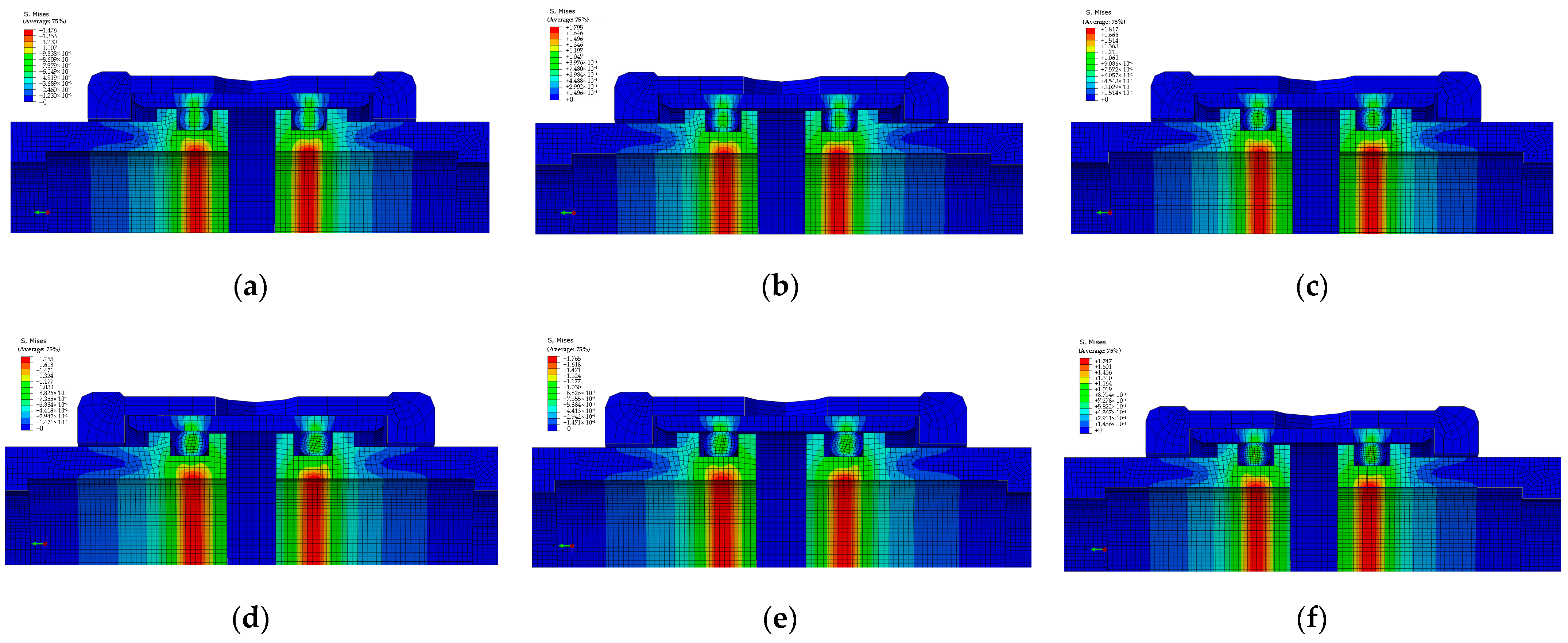
| Name | Element Number | Number of Mesh Nodes | Mesh Quality |
|---|---|---|---|
| Outer joint | 107,150 | 143,756 | No warning and error |
| Inner joint | 173,050 | 211,840 | No warning and error |
| Support block | 3272 | 4968 | No warning and error |
| Name | Section Diameter d1 (mm) | Height after Compression d2 (mm) | Friction Surface Diameter D (mm) |
|---|---|---|---|
| Outer joint | 3.52 | 2.94 | 47.304 |
| Inner joint | 1.78 | 1.43 | 14.757 |
| Frequency (Hz) | Tensile Stiffness (N/mm) | Compressive Stiffness (N/mm) | Slide Damping (N/(mm·s−1)) | Rotational Stiffness (N·mm/rad) | Rotational Damping (N·mm/(rad·s−1)) | Torsional Rigidity (N·mm/rad) | Torsional Damping (N·mm/(rad·s−1)) |
|---|---|---|---|---|---|---|---|
| 20 | 545.10 | 858.22 | 0.0101 | 146,727.73 | 13.043 | 125,595.29 | 33.07 |
| 30 | 525.45 | 913.91 | 0.0177 | 140,404.97 | 19.422 | 111,308.34 | 28.65 |
| 40 | 551.65 | 820.28 | 0.0173 | 143,151.33 | 17.316 | 121,308.36 | 29.59 |
| Average value | 540.73 | 864.14 | 0.0150 | 143,427.84 | 16.593 | 119,404.99 | 30.44 |
| Frequency (Hz) | Tensile Stiffness (N/mm) | Compressive Stiffness (N/mm) | Slide Damping (N/(mm·s−1)) | Rotational Stiffness (N·mm/rad) | Rotational Damping (N·mm/(rad·s−1)) | Torsional Rigidity (N·mm/rad) | Torsional Damping (N·mm/(rad·s−1)) |
|---|---|---|---|---|---|---|---|
| 20 | 38.17 | 119.48 | 0.0012 | 346.75 | 3.10 | 888.94 | 3.08 |
| 30 | 39.32 | 123.06 | 0.0014 | 357.15 | 3.19 | 915.61 | 2.99 |
| 40 | 37.02 | 115.90 | 0.0012 | 336.65 | 3.01 | 862.47 | 3.17 |
| Average value | 38.17 | 119.48 | 0.0013 | 346.85 | 3.10 | 889.01 | 3.09 |
| Kx (N/m) | Ky (N/m) | Kz (N/m) | Kτx (N·m/rad) | Kτy (N·m/rad) | Kτz (N·m/rad) |
|---|---|---|---|---|---|
| 2.38 × 10⁸ | 2.38 × 10⁸ | 2.38 × 10⁸ | 1.53 × 10⁴ | 8.42 × 10⁴ | 1.53 × 10⁴ |
| Cx (N·s/m) | Cy (N·s/m) | Cz (N·s/m) | Cτx (N·m·s/rad) | Cτy (N·m·s/rad) | Cτz (N·m·s/rad) |
|---|---|---|---|---|---|
| 4.66 × 10⁹ | 4.66 × 10⁹ | 4.66 × 10⁹ | 1.06 × 10⁵ | 6.97 × 10⁵ | 1.06 × 10⁵ |
| Name | Density (Tone/mm3) | Elastic Modulus (MPa) | Poisson Ratio |
|---|---|---|---|
| Inner and outer pipes Sleeve Inner and outer socket Support block | 7.92 × 10⁻⁹ | 199,950 | 0.27 |
| Clamp metal part Bracket | 2.73 × 10⁻⁹ | 73,100 | 0.33 |
| Nuts and bolts | 7.85 × 10⁻⁹ | 200,000 | 0.28 |
| Material Parameter | Value | Geometric Parameter | Value | Geometric Parameter | Value |
|---|---|---|---|---|---|
| Air volume modulus of elasticity (MPa) | 0.142 | L1 (mm) | 75.38 | L8 (mm) | 9.10 |
| Air density (kg/m3) | 1.29 | L2 (mm) | 376.87 | L9 (mm) | 7.74 |
| Plug quality (kg) | 0.003 | L3 (mm) | 6.06 | L10 (mm) | 9.88 |
| Sensor quality (kg) | 0.006 | L4 (mm) | 13.92 | L11 (mm) | 13.92 |
| - | - | L5 (mm) | 9.88 | L12 (mm) | 6.06 |
| - | - | L6 (mm) | 7.74 | L13 (mm) | 376.87 |
| - | - | L7 (mm) | 9.10 | L14 (mm) | 75.38 |
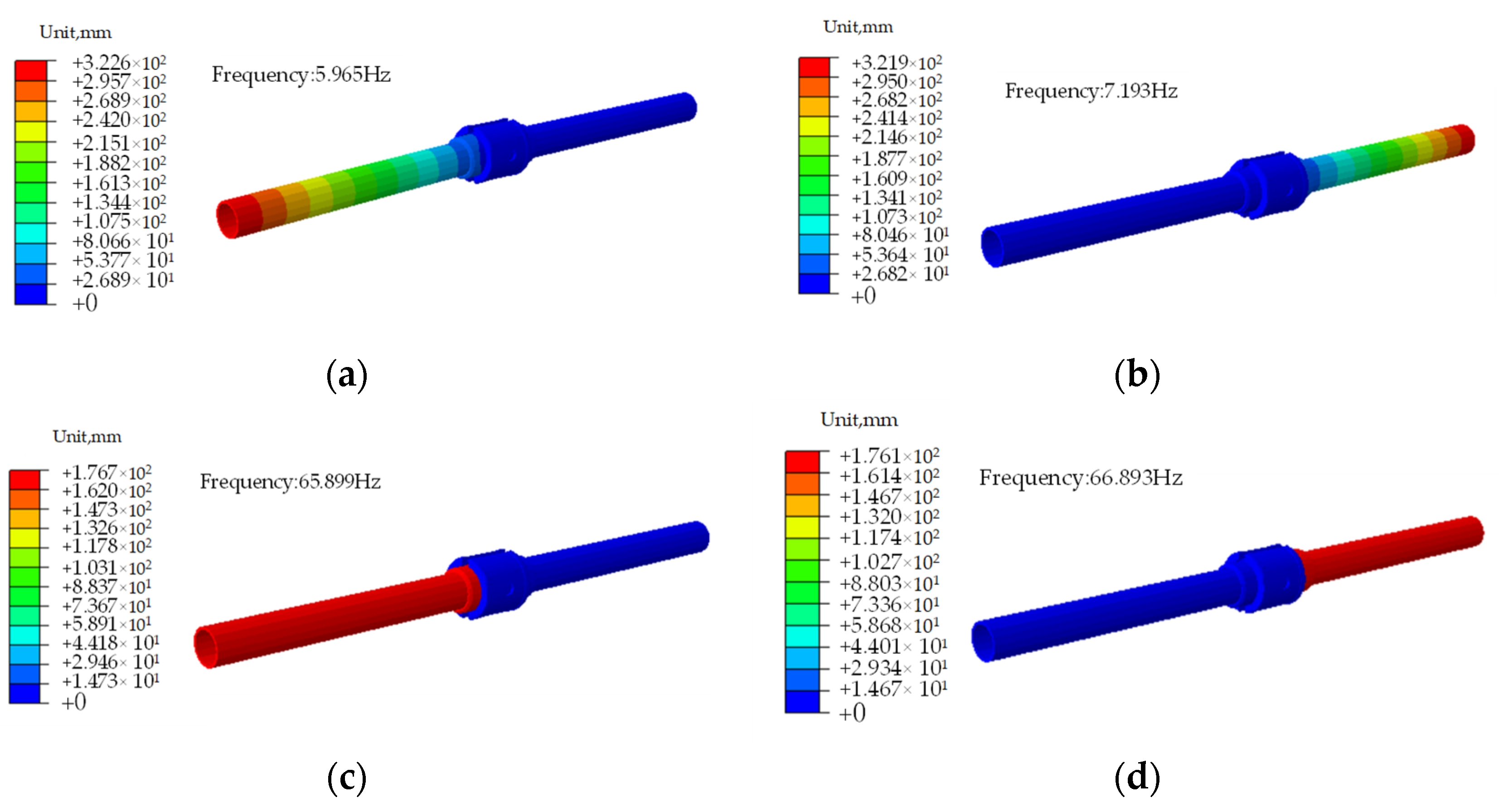
| Order | fn1 | fn2 | fn3 | fn4 | fn5 | fn6 |
|---|---|---|---|---|---|---|
| Test (Hz) | 1.978 | 4.527 | 8.967 | 18.152 | 40.910 | 83.345 |
| Numerical analysis (Hz) | 1.791 | 4.776 | 9.341 | 16.923 | 37.988 | 80.184 |
| Error | 9.45% | 5.50% | 4.17% | 6.77% | 7.14% | 3.79% |
Disclaimer/Publisher’s Note: The statements, opinions and data contained in all publications are solely those of the individual author(s) and contributor(s) and not of MDPI and/or the editor(s). MDPI and/or the editor(s) disclaim responsibility for any injury to people or property resulting from any ideas, methods, instructions or products referred to in the content. |
© 2023 by the authors. Licensee MDPI, Basel, Switzerland. This article is an open access article distributed under the terms and conditions of the Creative Commons Attribution (CC BY) license (https://creativecommons.org/licenses/by/4.0/).
Share and Cite
Quan, L.; Fu, C.; Yao, R.; Guo, C. Dynamic Modeling and Parameter Identification of Double Casing Joints for Aircraft Fuel Pipelines. Processes 2023, 11, 2767. https://doi.org/10.3390/pr11092767
Quan L, Fu C, Yao R, Guo C. Dynamic Modeling and Parameter Identification of Double Casing Joints for Aircraft Fuel Pipelines. Processes. 2023; 11(9):2767. https://doi.org/10.3390/pr11092767
Chicago/Turabian StyleQuan, Lingxiao, Chen Fu, Renyi Yao, and Changhong Guo. 2023. "Dynamic Modeling and Parameter Identification of Double Casing Joints for Aircraft Fuel Pipelines" Processes 11, no. 9: 2767. https://doi.org/10.3390/pr11092767
APA StyleQuan, L., Fu, C., Yao, R., & Guo, C. (2023). Dynamic Modeling and Parameter Identification of Double Casing Joints for Aircraft Fuel Pipelines. Processes, 11(9), 2767. https://doi.org/10.3390/pr11092767