Research on Downhole Throttling Characteristics of Gas Wells Based on Multi-Field and Multi-Phase

Abstract

The formation of natural gas hydrates seriously affects the production efficiency of gas wells. Obtaining the correct temperature and pressure profile along the wellbore of gas wells is a prerequisite for accurately predicting the location of hydrate formation and using downhole throttling technology. According to the numerical iterative transfer law of wellbore microelement state parameters, a multi-field and multi-phase coupling method is proposed. Based on the analysis of typical temperature and pressure models, considering the gas well velocity field and density field, a gas well multi-phase correction coefficient is introduced. Based on the judgment method of multi-phase flow pattern, the friction gradient equation of multi-phase flow is obtained, and the respective theoretical prediction equations are created for the temperature field, pressure field, density field, and velocity field. Thereby, a wellbore temperature and pressure field model with multi-field and multi-phase coupling is established. The model was applied to K1 and K2 gas wells, and the calculation results of the research model were compared with the PIPESIM simulation results and measured values. At the same time, the mean μ, variance σ, and the coefficient of variation C_m were evaluated, and the results show that the coefficient of variation of the calculation results of this research model is less than 15%, which indicates greater accuracy than the PIPESIM simulation results. These findings provide a theoretical basis for the design of wellbore structures and the use of downhole tools.

1. Introduction

In the oil and gas industry, wellbore structure design, use of downhole tools, and dynamic detection of gas wells, wellbore temperature and pressure field data are required so as to obtain reasonable wellbore structure and design parameters to ensure the safety and normal production of the wellbore [1]. In the process of natural gas extraction, with changes in wellbore temperature and pressure, hydrates may form, blocking the wellbore and pipelines and seriously affecting the production efficiency of the gas well [2]. At present, for the problem of hydrate plugging, downhole throttling technology is mainly used to prevent hydrate formation. Therefore, it is necessary to clarify the temperature and pressure distribution of gas wells, predict the location of hydrate formation, apply downhole throttling technology to prevent hydrate formation, design the diameter of the throttling nozzle and select the right location for the throttle. Ramey [3], using the energy conservation and momentum conservation equations, ignored the heat loss along the wellbore direction, simplified the formula for calculating the heat transfer between the wellbore and the formation using dimensionless time, and proposed a wellbore temperature field calculation model for the first time. Tragesser [4] proposed, for the first time, a method for calculating the actual cementing temperature and the wellbore temperature during the mud circulation process. Based on the semi-steady-state algorithm, a calculation method for the temperature field of the casing and tubing–casing annulus at different times was proposed. Hu [5] proposed, for the first time, a detailed calculation formula for the natural convection and radiation heat transfer coefficients in the tubing–casing annulus. Raymond [6] first proposed a theoretical model to calculate the temperature field with the full transient method. Han et al. [7] proposed a two-dimensional transient model of wellbore temperature based on the precise short-time integration method in the single-point subdomain. Their model provides accurate temperature parameters for the precise mechanical analysis of the wellbore columns and the safety evaluation of well integrity. Fu et al. [8] established the governing equation of the wellbore temperature field in the wellbore under the condition of thermal insulation tubing, constructed a wellbore temperature distribution model, and clarified the comprehensive heat transfer coefficient between the inner radius of the wellbore and the outer radius of the casing. Duns et al. [9] proposed a predictable gas–liquid two-phase pipe flow pressure model based on laboratory simulation data and field data correction. Hagendorn et al. [10] proposed a gas–liquid two-phase pipe flow pressure model, which can solve the problems of the friction coefficient and liquid holdup of the gas–liquid mixture. Bhagwat et al. [11] established a gas–liquid two-phase drift-flux model to calculate the gas holdup without judging the flow pattern.

The physical properties of the fluid in the wellbore of a gas well will change with the temperature and pressure, and the temperature and pressure will affect each other. Zhang et al. [12], considering the Joule–Thomson effect, established a fully transient wellbore temperature–pressure coupling model, and used the fourth-order Runge–Kutta method to predict the temperature and pressure of natural gas at different well depths. Hasan et al. [13,14] considered the convection heat transfer in the tubing–casing annulus and the Joule–Thomson effect together with the convection heat transfer between air and seawater in offshore oil wells, and established a comprehensive wellbore–reservoir model which can calculate the two-phase flow pressure transient behavior and fluid temperature throughout the wellbore. Xu et al. [15] considered the enthalpy as a function of pressure and temperature. In their proposed coupled transient wellbore–reservoir thermal model, Onur et al. [16] considered Joule–Thomson heating or cooling, thermal insulation fluid expansion, conduction, and convection effects in the formation part, while in the transient wellbore part, friction and gravity effects were considered. Wang [17] obtained the Fanning friction coefficient by applying the semi-transient method and Colebrook formula, calculated the temperature profile, and established a wellbore temperature–pressure coupling model. Zhang et al. [18], based on thermodynamic theory, considered mechanical and hydraulic heat sources, solved the equations by the fully implicit finite difference method and matrix pursuit method, and proposed a calculation model of the drilling temperature and pressure field for shale gas horizontal wells. Zheng et al. [19] combined the wellbore heat transfer mechanism and the calculation method of pipe flow pressure drop gradient through transient analysis by considering the interaction between fluid physical parameters and temperature and pressure. Thereby, they established a wellbore pressure coupling model for water-bearing gas wells and solved the problem that commonly used temperature and pressure models can only be used for single-phase states under complex well conditions.

Dastkhan et al. [20,21] proposed a numerical simulation method for the transient change of formation pressure and temperature by simultaneously coupling and solving the fluid flow and energy equations. They simulated the change in pressure and temperature distribution in the reservoir with time, and analyzed the influence of formation pressure and temperature by changing rock and fluid properties. Liu et al. [1] established a single-phase gas transient flow temperature–pressure coupling mathematical model of the fluid in the wellbore during gas well production. The comparison with the field measured data and the calculation results of the analytical model showed that the coupling model has higher accuracy.

In summary, the temperature and pressure field calculation methods proposed for different well conditions and different well testing and completion are relatively mature. They mainly include the correction of the classic temperature field model, the calculation and correction of the heat transfer coefficient, the solution of the temperature field in the production, drilling and water injection states, and the research of the deep-sea temperature field. At present, most models only consider the effects of the temperature field, pressure field, single-phase flow, or gas–liquid two-phase flow, and ignore the effects of the velocity field, density field, sand content, and oil content. Therefore, in order to accurately predict the distribution of wellbore temperature and pressure, a multi-field and multi-phase coupled gas well temperature and pressure field model was developed in this study.

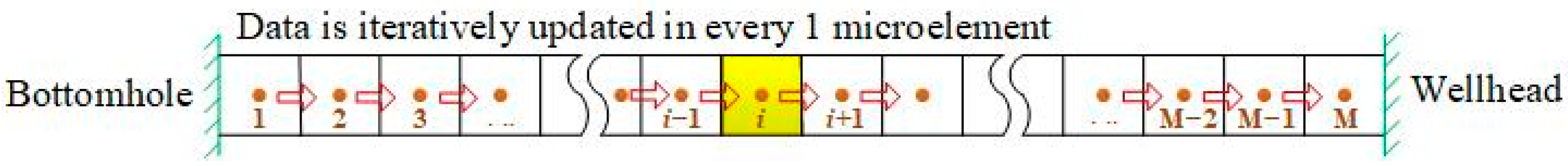
2. Construction of Wellbore Temperature and Pressure Field Model with Multi-Field and Multi-Phase Coupling

The gas well multi-field and multi-phase model is a theoretical model for wellbore parameter prediction. Based on the wellbore model assumption, the gas state equation, mass conservation, momentum conservation, and energy conservation, the theoretical calculation model is obtained through wellbore parameter coupling.

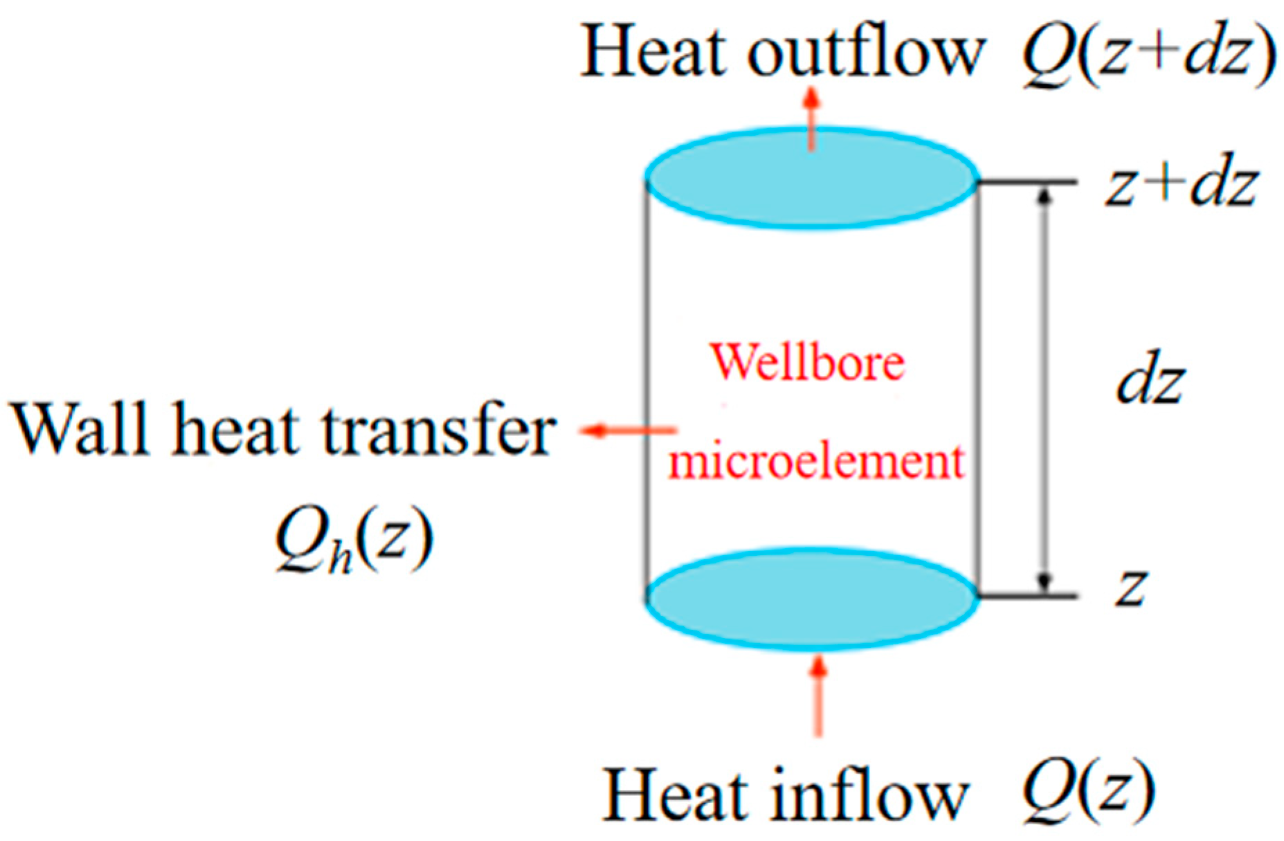
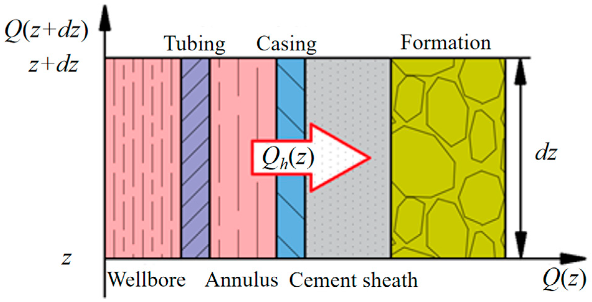
2.1. Basic Assumptions of the Model

The half-section of the wellbore structure diagram is shown in Figure 1. The center of the wellbore structure is the tubing, inside of which from the center of wellbore to outside, are the production tubing, tubing annus, technical casing, tubing annus, surface casing, cement sheath, conductor, cement sheath and formation. The tubing annus is filled with annus fluid. It can be seen from Figure 1 that in the wellbore structure, the wellbore structural components such as tubing, casing, and cement sheath are connected through “rings” to form a solid gas production wellbore, so as to ensure that natural gas can be safely transported from the formation to the ground.

In order to further construct a multi-field and multi-phase coupled gas well temperature and pressure field model, the following assumptions are made:

(1)

It is assumed that the heat transfer from the wellbore to the formation around the wellbore is radial.

(2)

It is assumed that the conduction process of heat from the wellbore to the formation is unsteady and that the heat transfer in the wellbore is steady state.

(3)

There is only radial heat loss in the wellbore micro-elements.

(4)

The gas–water/gas–solid two-phase transient in the wellbore satisfies the thermal equilibrium [22].

(5)

During the flow process, the fluid and the outside world do not perform work on each other.

(6)

The proportion of the gas phase in the fluid is much higher than that of other phases [23].

(7)

Each phase in the fluid is composed of continuous particles and conforms to the theory of continuous media, which can be averaged in time and space.

(8)

There is no mass transfer between the components.

(9)

The fluid flow in the wellbore is regarded as a one-dimensional flow along the wellbore axis.

(10)

All components on the same cross-section are in thermal equilibrium, and all components have the same pressure and temperature.

2.2. Multi-Phase Coupling Method

The microelement method is used to divide the wellbore into small segments of microelements, as shown in Figure 2. We input the initial parameters, iteratively calculate each small segment, and complete the calculation of the entire well depth structure. We then apply the obtained parameters in each small segment of the calculation to the next stage of calculation, thereby achieving coupling of the wellbore parameters.

It is assumed that the fluid in the wellbore of a gas well contains a variety of substances: gas (represented by subscript q), water (represented by subscript w), oil (represented by subscript y), sand (represented by subscript s), and gas hydrate (represented by the subscript t). Then the volume fraction of natural gas is V_q(z), the volume fraction of water is V_w(z), the volume fraction of oil is V_y(z), the volume fraction of sand is V_s(z), and the volume fraction of gas hydrate is V_t(z).

The calculation method for mixture density is as follows:

$${\rho }_m=V_q{\rho }_q+V_w{\rho }_w+V_y{\rho }_y+V_s{\rho }_s$$

(1)

2.3. Judgment of Multi-Phase Flow Pattern and Establishment of Flow Friction Gradient Equation

Compared with the gas–liquid–solid three-phase flow pattern and the gas well single-phase flow, the fundamental difference lies in the pressure fluctuation inside the wellbore [24]. However, the multi-phase flow friction gradient of the fluid mixture in the wellbore is closely related to the flow pattern [25]. Therefore, in order to detect the pressure change of the multi-phase flow, it is necessary to determine the calculation method of the friction pressure drop gradient under different flow patterns:

(1)

Bubble flow

The gas–solid phase is the dispersed phase, and the liquid phase is the continuous phase. Its existence condition are as follows:

When the fluid flows at medium or low speeds:

$$v_t<v_{tT} \mathrm{and} v_q<0.249v_y+0.357v_t$$

(2)

When the fluid flow rate is high, the fluid is in a dispersed bubbly flow state:

$${\alpha }_g>0.52 \mathrm{and} v_m>5.88d_h^{0.48}{\left[\frac{\left({\rho }_s-{\rho }_q\right)g}{\sigma }\right]}^{0.5}{\left[\frac{\sigma }{{\rho }_s}\right]}^{0.6}{\left[\frac{{\rho }_m}{{\mu }_y}\right]}^{0.08}$$

(3)

$$v_t=1.53\times {\left[g\sigma \left({\rho }_s-{\rho }_q\right)/{\rho }_s^2\right]}^{0.25}$$

$$v_{tT}=0.35{\left[g{d}_h\left({\rho }_s-{\rho }_g\right)/{\rho }_s\right]}^{0.5}$$

The friction coefficient is expressed as:

$$\frac{1}{\sqrt{f_m}}=-4\lg \left[\frac{\epsilon /d_h}{3.7065}-\frac{5.0452\log A}{Re}\right]$$

(4)

where $Re=\frac{d_h{v}_m{\rho }_m}{{\mu }_m}$, $A=\frac{{\left(\epsilon /d_h\right)}^{1.1098}}{2.8257}-{\left(\frac{7.149}{Re}\right)}^{0.8981}$.

The frictional pressure drop is expressed as:

$${\left(\frac{dp}{dz}\right)}_{fr}=\frac{f_m{v}_m^2{\rho }_m}{2d_h}$$

(5)

(2)

Slug flow

When the flow pattern changes to slug flow, the flow instability strengthens. Its existence conditions are as follows:

$$v_q>0.249v_y+0.357v_t$$

(6)

$$\{\begin{array}{c}{\rho }_q{v}_y^2<17.1\times lg{\left({\rho }_y{v}_y\right)}^2-23.21, {\rho }_y{v}_y^2>50\\ {\rho }_q{v}_y^2<0.00673{\left({\rho }_y{v}_y^2\right)}^{1.7}, {\rho }_y{v}_y^2>50\end{array}$$

(7)

The calculation of the friction coefficient is consistent with that of the bubble flow, and the friction pressure drop is expressed as:

$${\left(\frac{dp}{dz}\right)}_{fr}=\frac{f_m{v}_m^2{\rho }_m}{2d_h}\left(1-{\alpha }_q\right)$$

(8)

(3)

Foam flow

The fluid in the tube has strong turbulence, the large bubbles are broken up into small foams, and the liquid and gas move up rapidly together. Compared with the slug flow, the foam flow is more intense. Its existence conditions are as follows:

$$v_q<3.1\times {\left[g\sigma \left({\rho }_s-{\rho }_q\right)/{\rho }_s^2\right]}^{0.25}$$

(9)

$$\{\begin{array}{c}{\rho }_q{v}_y^2>17.1\times lg{\left({\rho }_y{v}_y\right)}^2-23.21, {\rho }_y{v}_y^2>50\\ {\rho }_q{v}_y^2>0.00673{\left({\rho }_y{v}_y^2\right)}^{1.7}, {\rho }_y{v}_y^2>50\end{array}$$

(10)

The calculation of the friction coefficient and friction pressure drop is consistent with that of slug flow.

(4)

Annular flow

The gas enters the pipe in the form of a jet at a very high flow rate, and a layer of liquid film forms along the inner wall of the pipe. At this time, the relative motion between the gas and other phases is small, and the existence conditions are:

$$v_q>3.1\times {\left[g\sigma \left({\rho }_s-{\rho }_q\right)/{\rho }_s^2\right]}^{0.25}$$

(11)

The friction pressure drop is calculated as follows:

$${\left(\frac{dp}{dz}\right)}_{fr}=\frac{2f_c{v}_q^2{\rho }_c}{d_h}$$

(12)

$$f_c=\frac{0.079\times \left[1+75\times \left(1-{\alpha }_g\right)\right]}{R{e}^{0.25}}$$

(13)

$${\rho }_c=\frac{v_q{\rho }_q+EF{v}_y{\rho }_y}{v_q+EF{v}_y}$$

(14)

$$\{\begin{array}{c}EF=0.0055{\left[{\left(v_q\right)}_c\times {10}^4\right]}^{2.86}, {\left(v_q\right)}_c\times {10}^4<4\hfill \\ EF=0.857\lg \left[{\left(v_q\right)}_c\times {10}^4\right]-0.20, {\left(v_q\right)}_c\times {10}^4>4\end{array}$$

(15)

$${\left(v_q\right)}_c=v_q{\mu }_q{\left({\rho }_q/{\rho }_y\right)}^{0.5}/\sigma$$

(16)

where v_q, v_y, and v_t are the apparent phase velocity of gas and liquid and limiting rising velocity of bubble (m/s); v_tT is the Taylor bubble rising velocity (m/s); d_h is the hydraulic diameter (m); σ is the gas–liquid interface tension (N/m); μ_y is the liquid phase viscosity (MPa·s); and ε is the pipe wall roughness (m).

2.4. Multi-Field Coupling Model Construction

In the process of natural gas extraction, the physical properties of the fluid in the wellbore change with temperature, pressure, velocity, and density, and the temperature, pressure, velocity, and density affect each other. In order to accurately predict the distribution of wellbore temperature and pressure, a multi-field coupling model is established.

(1)

Temperature field

To create a theoretical model for the segmented wellbore structure, we take the bottom of the wellbore as the origin of the coordinates, take the Z direction as the positive direction, and assign micro-elements of length dz on the tubing, as shown in Figure 3. We then start calculation from the bottom of the well to the wellhead.

As shown in Figure 4, part of the energy flowing into the wellbore microelement flows out along the axial direction, while the rest of energy dissipates radially into the formation through the wall:

$$Q(z)=Q(z+dz)+Q_h(z)$$

(17)

The heat flowing into the microelement can be expressed as:

$$Q(z)=w{C}_{p}T(z)$$

(18)

The heat flowing out of the microelement can be expressed as:

$$Q(z+dz)=w{C}_{p}T(z+dz)$$

(19)

The radial heat transfer of fluid along the microelement is:

$$Q(z)=2\pi r_{to}{U}_{to}(T_h-T)dz$$

(20)

Therefore, the energy conservation equation can be expressed as:

$$w{C}_{p}dT/dz=2\pi r_{to}{U}_{to}(T_h-T)$$

(21)

We consider the radial and axial heat dissipation of the fluid element in Figure 3 as equivalent. Therefore:

$$T_h=\frac{k_z{T}_z+r_{to}{U}_{to}Tf(t)}{k_z+r_{to}{U}_{to}f(t)}$$

(22)

We substitute into the energy conservation equation to obtain:

$$w{C}_{p}dT/dz=\frac{2\pi r_{to}{U}_{to}{k}_z(T_z-T)}{k_z+r_{to}{U}_{to}f(t)}$$

(23)

We define:

$$a=\frac{C_{p}w}{2\pi }\left(\frac{k_z+r_{to}{U}_{to}f(t)}{r_{to}{U}_{to}{k}_z}\right)$$

(24)

Then, it can be concluded that

$$\frac{dT}{dz}+\frac{T}{a}-\frac{T_z}{a}=0$$

(25)

It is known that $T_z=T_d-g_{e}z$.

Solving the equation gives:

$$T=C_1{e}^{-z/a}+T_d+(a-z)g_e$$

(26)

Substituting the initial condition z = z(0), T = T(0) into the solution, we obtain:

$$C_1=\frac{T(0)+T_d+(a-z)g_e}{e^{-z(0)/a}}$$

(27)

We then introduce the Joule–Thomson coefficient C_J. For the fluid element dz of the wellbore, the following equation is derived according to the energy conservation equation:

$$\frac{dT}{dz}=\frac{f(t)-T_z}{b}-\frac{g}{C_p}+C_J\frac{dp}{dz}-\frac{vdv}{g_e{C}_p}$$

(28)

where

$$b=\frac{C_{p}w}{2\pi }\left(\frac{k_z+r_{to}{U}_{to}f(t)}{r_{to}{U}_{to}{k}_z}\right)$$

Integrating the equation solves:

$$T_{out}=T_z+b\left(1-e^{\Delta z/b}\right)\left(-\frac{g}{C_p}+C_J\frac{dp}{dz}-\frac{vdv}{C_{p}dz}+g_e\right)+e^{\Delta z/b}(T_{in}-T_z)$$

(29)

where T_in, T_out, and T_z are the wellbore fluid temperature at the inlet and outlet of the wellbore microelement, and the formation temperature at the inlet, °C; Δz is the depth of the microelement well section, m; g is the gravitational acceleration, m/s²; C_J is the Joule–Thomson coefficient, K/MPa; g_e is the geothermal gradient, K/m; C_p is the change with pressure, J/(kg·K); w is the mass flow rate of natural gas, kg/s; U_to is the total heat transfer coefficient of the wellbore, W/(m²·K); r_to is the outer radius of the tubing, m; k_z is the thermal conductivity of the formation, W/(m·K); and f(t) is the transient heat transfer function, which is dimensionless.

(2)

Pressure field

For single-phase flow, according to the law of conservation of momentum and considering the change in kinetic energy gradient in the calculation process, the pressure drop of a vertical well can be expressed as:

$$\frac{d{p}_z}{dz}=-\rho g-\frac{f\rho v^2}{2d}-\frac{\rho vdv}{dz}$$

(30)

Similarly, the momentum conservation equation of homogeneous flow can be expressed as:

$$\frac{d{p}_z}{dz}=-\left(\frac{d{p}_g}{dz}\right)-\left(\frac{d{p}_f}{dz}\right)-\left(\frac{d{p}_a}{dz}\right)=-{\rho }_{m}g-\frac{f_m{\rho }_m{v}^2}{2d}-\frac{Gd{R}_m}{dz}$$

(31)

where ρ_m is the homogeneous flow density, kg/m³; f_m is the two-phase flow Fanning friction coefficient, which is dimensionless; G is the mass flow rate, kg/(m²·s); and R_m is the two-phase flow specific volume, kg/m³.

The equation for solving the Fanning friction coefficient is:

$$\frac{1}{\sqrt{f_m}}=1.14-2\mathit{log}\left[\frac{e}{D}+\frac{21.25}{{\mathit{Re}}^{0.9}}\right]$$

(32)

In addition, referring to the empirical formula for the pressure drop in gas carrying water and sand in the application of air drilling, the flow pressure p at the depth h of the gas–liquid–solid three-phase flow in the wellbore of a gas well can be obtained by the following equation:

$$\begin{array}{l}144b(p_z-p_{jk})+\frac{1-2bm}{2}\ln \left|\frac{{(144p_z+m)}^2+n}{{(144p_{jk}+m)}^2+n}\right|-\\ \frac{m+\frac{b}{c}n-b{m}^2}{\sqrt{n}}\left[{\tan }^{-1}\left(\frac{144p_z+m}{\sqrt{n}}\right)-{\tan }^{-1}\left(\frac{144p_{jk}+m}{\sqrt{n}}\right)\right]\\ =a(1+d^{2}e)h\end{array}$$

(33)

where

$$a=\frac{23.59S_s{Q}_s+870.42S_l{Q}_l+33.82S_g{Q}_g}{1000T_z{Q}_g}$$

$$b=\frac{0.442Q_s+13.96Q_l}{1000T_z{Q}_g}$$

$$c=\frac{2.966\times {10}^{-6}{T}_z{Q}_g}{\pi r_{ti}^2}$$

$$d=\frac{5.076\times {10}^{-4}{Q}_s+0.016Q_l}{600\pi r_{ti}^2}$$

$$e=\frac{64.58f}{g{d}_{ti}}$$

$$f={\left[\frac{1}{1.74-2\lg \left(\frac{65.62\epsilon }{d_{ti}}\right)}\right]}^2$$

$$m=\frac{cde}{1+d^{2}e}$$

$$n=\frac{c^{2}e}{{\left(1+d^{2}e\right)}^2}$$

where p_z is the flow pressure at the calculation point, Pa; p_jk is the wellhead flow pressure, Pa; r_ti is the inner radius of the tubing, m; d_ti is the inner diameter of the tubing, m; h is the well depth, m; ε is the absolute roughness of the tubing wall, m; S_s is the weight of sand particles, kgf/m³; S_l is the weight of water, kgf/m³; S_g is the weight of gas, kgf/m³; Q_g is the gas production rate, m³/s; Q_l is the water production rate of the gas, m³/s; Q_s is the sand production rate, m³/s; and T_z is the temperature at the calculation point, K.

(3)

Density field

The known gas state equation is

$$pV=\frac{m}{M}ZRT$$

(34)

And ρ = m/V, so for each fluid element, we obtain:

$$\rho =\frac{Mp(z)}{RT(z)Z(z)}$$

(35)

As shown in Equation (35), the density field is calculated based on the temperature and pressure field and other wellbore parameters.

(4)

Velocity field

According to the conservation of mass,

$$\rho \frac{d\upsilon }{dz}+\upsilon \frac{d\rho }{dz}=0$$

(36)

Therefore,

$$v=e^{C_1+\ln \rho \left(z\right)}$$

(37)

Substituting the initial conditions v = v(0) and ρ = ρ(0) into the equation we obtain:

$$v=e^{\ln \frac{\rho \left(z\right)v(0)}{\rho (0)}}$$

(38)

As shown in Equation (38), the fluid velocity is calculated from the fluid density since the density field is related to the temperature and pressure field. In summary, the temperature–pressure–velocity–density field coupling calculation model has been created.

3. Case Study of Wellbore Temperature and Pressure Field Model with Multi-Field and Multi-Phase Coupling

(1)

Example calculation

In order to verify the reliability of the model, calculation and analysis of wells K1 and K2 were carried out. The basic wellbore parameters of the two wells are shown in

Table 1. K1 and K2 wellbore parameters.

Basic Parameters	K1	K2
Inner diameter of tubing (mm)	62	76
Tubing wall thickness (mm)	7	6.5
Tubing steel grade	N80	J55
Inner diameter of surface casing (mm)	157.08	226.62
Surface casing wall thickness (mm)	10.36	8.94
Setting depth of surface casing (m)	567.74	554.64
Inner diameter of gas layer casing (mm)	108.62	121.36
Gas layer casing wall thickness (mm)	9.19	9.17
Setting depth of gas layer casing (m)	2874.59	2486.47
Casing grade	P110	P110
Roughness of tubing casing wall (mm)	0.0254	0.0254
Wellbore diameter (mm)	431.8	445.6
Artificial bottom hole (m)	2867.08	2472.3
Gas production (m3/d)	3.3562 × 104	5.122 × 104
Water production (m3/d)	2.4	64.025
Sand production (m3/d)	1.2	0.8
Oil production (m3/d)	0.2	0.04
Bottom hole pressure (MPa)	20.332	18.5
Bottom hole temperature (°C)	92.776	65
Geothermal gradient (°C/m)	0.0275	0.024
Total heat transfer coefficient (J/(m2·s·°C))	11.356	10.564
Formation thermal diffusion coefficient (m2/s)	7.5 × 10−7	7.5 × 10−7
Formation thermal conductivity (J/(m·s·°C))	1.7307	1.7297
Relative density of natural gas	0.5756	0.5916

.

The above data were imported into PIPESIM software (2022.1.700×64). The wellbore structure, which is shown in Figure 5, consists of the fluid in the tubing, tubing, gas layer casing, surface casing, annular fluid, and cement sheath.

Substituting the basic data of wells K1 and K2 into the Matlab coupling model and PIPESIM software, respectively, the calculation results of the wellbore state parameters of the two wells can be obtained, as shown in Figure 6 and Figure 7:

It can be seen from Figure 6 and Figure 7 that when the gas well is in the production stage and the wellbore fluid reaches the surface from the bottom of the wellbore, the wellbore temperature and pressure of the two gas wells decrease linearly as the well depth decreases. The reason for this phenomenon is that, compared with the wellhead, the bottom of the well is in a high-temperature and high-pressure environment. During the process of formation fluid flowing out of wells K1 and K2, heat is transferred to the surrounding formations. When the gas well production reaches a steady state, the trend of heat transfer from the wellbore to the formation reaches a steady state, so the wellbore temperature and pressure tend to change in the geothermal gradient. In addition, it can be seen from the figure that the calculation model proposed in this study is closer to the measured value than the calculation model of PIPESIM, so the calculation model proposed in this study is more accurate.

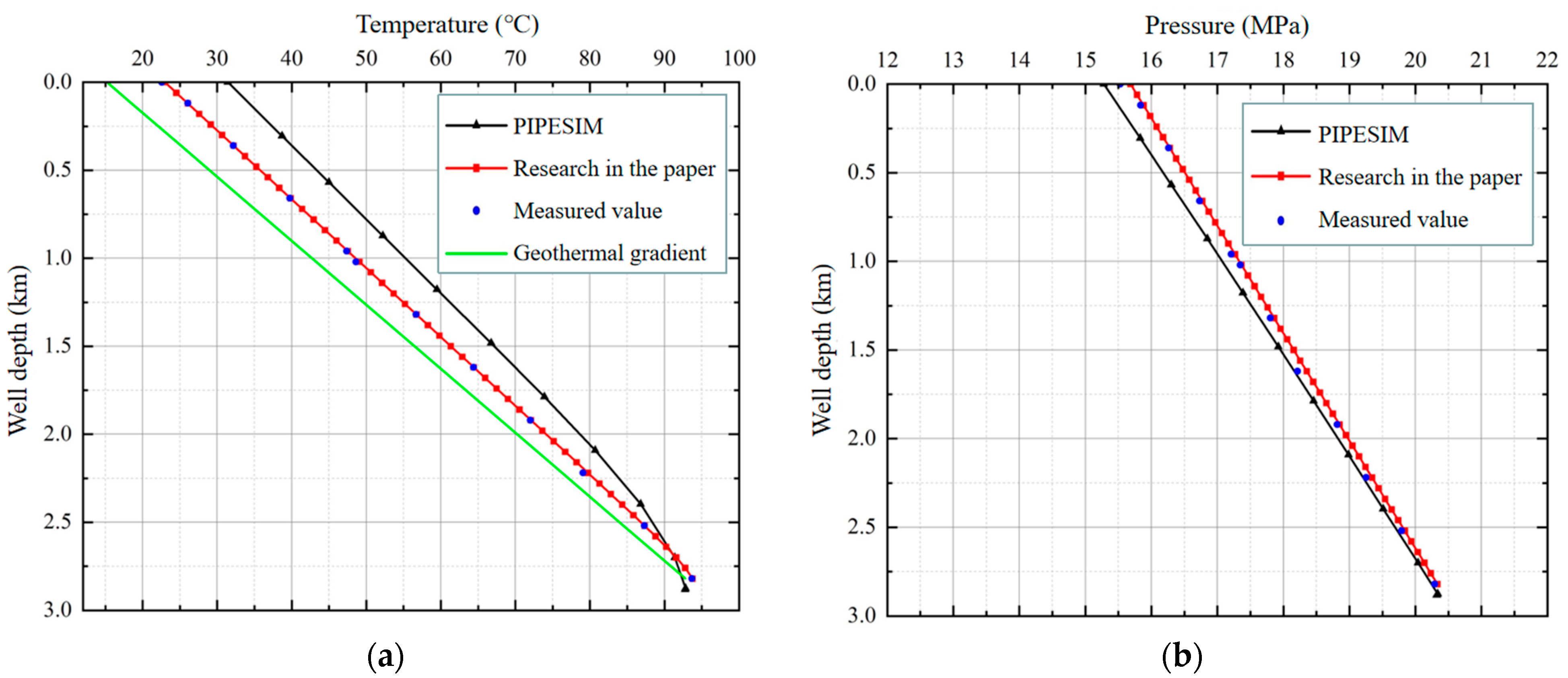
(2)

Error analysis

In order to verify the accuracy of the multi-field and multi-phase coupling model, considering the different dimensions and well conditions of the temperature and pressure calculation results of K1 and K2 wells, the deviation of the result variables relative to the field measured data is measured by comparing the variation coefficient C_m of the result variables.

The variation coefficient can be obtained by the following equation:

$$C_m=\frac{\sigma }{\mu }$$

(39)

where C_m is the variation coefficient, σ is the standard deviation, and μ is the mean value, all of which are dimensionless.

By solving the coefficient of variation of the four groups of results in Figure 6 and Figure 7, the variation coefficient is obtained, as shown in Figure 8 and Figure 9.

It can be seen from Figure 8 and Figure 9 that the variation coefficient C_m of each group of calculation result data of the wellbore temperature and pressure field model in this study based on multi-field and multi-phase coupling is less than 15%. The standard deviation and the mean values are smaller than the PIPESIM simulation results, indicating that the proposed model has better calculation accuracy.

4. Application of Multi-Field and Multi-Phase Coupling

4.1. Temperature and Pressure Changes before and after Throttling

The wellbore temperature before and after throttling can be solved by the temperature and pressure field model, and the temperature and pressure near the throttle nozzle can be solved by the throttle temperature drop and pressure drop model [26]. Throttling is a process of pressure and temperature drop. According to thermodynamic theory, assuming that the upstream pressure is p₁ and the downstream pressure is p₂, the critical pressure ratio is β_k = p₂/p₁ = (2/K + 1)^K/K−1. Here, K is the fluid adiabatic coefficient, which is dimensionless. Assuming that p₁ is constant, the gas at the gas nozzle produces two flow characteristics with the change in p₂, that is, when p₂/p₁ ≤ (2/K + 1)^K/K−1, the flow is in a critical flow state. When p₂/p₁ > (2/K + 1)^K/K−1, the flow is in a subcritical flow state [27].

(1)

Temperature drop

The throttle upstream temperature T₁ and throttle upstream pressure p₁ can be obtained through the multi-field and multi-phase coupling model, and the throttle downstream pressure p₂ can be obtained according to the expression of the critical pressure ratio β_k. Assuming that throttling is an isenthalpic process and introducing the Joule–Thomson coefficient, the throttle downstream temperature can be expressed as:

$$\Delta T=T_1-T_2=C_J\left(p_1-p_2\right)$$

(40)

where C_J is the Joule–Thomson coefficient, K/MPa; T₁ is the upstream temperature of the throttle nozzle, K; p₁ is the upstream pressure of the throttle nozzle, MPa; T₂ is the downstream temperature of the throttle nozzle, K; and p₂ is the downstream pressure of the throttle nozzle, MPa.

(2)

Pressure drop

The downhole safety valve formula [28,29] (SSSV) is used to calculate the throttle pressure drop at the throttle nozzle during subcritical flow. The upstream pressure p₁ of the throttle is obtained by the Hagedom–Brown vertical pipe pressure calculation method. By incorporating p₁ into the downhole safety valve formula, the pressure drop law formula can be obtained:

$$\Delta p=p_1-p_2=\frac{1.5{\gamma }_g{p}_1}{Z_1{T}_1}\left(1-{\beta }_d^4\right){\left[\frac{17.6447Z_1{T}_{1}Q}{p_1{d}^2{C}_{d}Y}\right]}^2$$

(41)

$$Y=1-\left[0.41+0.35{\beta }_d^4\right]\left(\frac{p_1-p_2}{k{p}_1}\right)$$

(42)

where Δp is the throttle pressure drop, MPa; β_d is the nozzle ratio, β_d = d/d_ti; γ_g is the relative density of natural gas, dimensionless; d_ti, d is the inner diameter of the tubing and diameter of the throttle nozzle, m; C_d is the flow coefficient, which is dimensionless and usually taken as 0.9; k is the natural gas adiabatic index, which is dimensionless and taken as 1.28; Y is the expansion coefficient, dimensionless (Y = 0.85, obtained by the iterative method); Q is the gas well production, m³/d; Z₁ is the gas compression factor under the conditions of T₁ and p₁, dimensionless; T₁ is the upstream temperature of the throttle nozzle, K; and p₁ is the upstream pressure of the throttle nozzle, MPa.

(3)

Calculation of minimum throttle nozzle diameter

The pressure drop Δp is obtained by solving Equation (41), and the throttle nozzle diameter d and the throttle critical flow rate Q are reversely calculated to design a reasonable nozzle diameter. Considering the principle of equal enthalpy for throttling, the relationship between the wellbore flow rate and the pressure ratio before and after throttling in the subcritical state is

$$Q=0.408p_1{d}^2\sqrt{\frac{k}{k-1}·\frac{1}{{\gamma }_g{T}_1{Z}_1}·\left({\beta }_k^{\frac{2}{k}}-{\beta }_k^{\frac{k+1}{k}}\right)}$$

(43)

There is a maximum flow in the state of critical flow:

$$Q_{\max }=0.408p_1{d}^2\sqrt{\frac{k}{k-1}·\frac{1}{{\gamma }_g{T}_1{Z}_1}·\left[{(\frac{2}{k+1})}^{\frac{2}{k-1}}-{(\frac{2}{k+1})}^{\frac{k+1}{k-1}}\right]}$$

(44)

where F_ss is the sand content and water content correction coefficient, which is dimensionless and can be determined through experiments; Q_c is the volume flow through the throttle nozzle, m³/d; d is the diameter of the throttle nozzle, m; p₁ is the upstream pressure of the throttle nozzle, MPa. T₁ is the upstream temperature of the throttle nozzle, K; k is the adiabatic index of natural gas, which is dimensionless and set at 1.28; and γ_g is the relative density of natural gas, dimensionless.

Therefore, the reasonable equation for calculating nozzle diameter is:

$$d={\left(\frac{Q_c{F}_{ss}{\gamma }_g{T}_1{Z}_1}{0.8605p_1\left({\beta }_k^{\frac{2}{k}}-{\beta }_k^{\frac{k+1}{k}}\right)}\right)}^{0.5}$$

(45)

(4)

Calculation of minimum depth of entry

Downhole throttling technology is used to readjust the temperature and pressure field in the wellbore. When the downstream fluid temperature is higher than the hydration generation temperature under the pressure condition after throttling, it can effectively prevent the generation of hydrates, that is, the temperature satisfies the equation:

$$T_2\ge T_h$$

(46)

where T_h and T₂ are the hydrate formation temperature and downstream fluid temperature, K.

The fluid temperature upstream of the throttle nozzle is slightly higher than the geothermal temperature at the same depth, namely:

$$T_1=T_{\Delta }+\frac{h_{\min }}{g_e}+T_0$$

(47)

where T_Δ is the difference between the fluid temperature before throttling and the geothermal temperature at the same depth, K; Z₁ is the gas compression factor under the conditions of T₁ and p₁, dimensionless; h_min is the minimum working depth of the throttle, m; T₀ is the wellhead average airflow temperature, K; and g_e is the geothermal gradient, m/K.

The temperature and pressure of the fluid during throttling have the following relationship:

$$\frac{T_2}{T_1}={\left(\frac{p_2}{p_1}\right)}^{Z_1\left(k-1\right)/k}$$

(48)

Through modification of the above equation, the temperature after throttling can be obtained:

$$T_2=T_1{\beta }_k^{Z_1\left(k-1\right)/k}$$

(49)

Substituting Equation (47) into Equation (49), we can calculate the downstream temperature of the throttle nozzle:

$$T_2=\left(T_{\Delta }+\frac{h_{\min }}{g_e}+T_0\right){\beta }_k^{Z_1\left(k-1\right)/k}$$

(50)

According to Equation (50), the calculation equation for the optimal depth of the downhole throttle device under the state of critical flow is as follows:

$$L_{\min }=g_e\left(T_h{\beta }_k^{Z_1(1-k)/k}-T_{\Delta }-T_0\right)$$

(51)

where L_min is the minimum depth of entry of the throttle, m; g_e is the geothermal gradient, m/K; Z₁ is the upstream natural gas compression factor, dimensionless; k is the natural gas adiabatic index, taken as 1.28; T_h is the hydrate formation temperature, K; T₀ is the average gas flow temperature at the wellhead, K; β_k is the critical pressure ratio, dimensionless; and T_Δ is the difference between the fluid temperature before throttling and the geothermal temperature at the same depth, K.

When calculating the optimal depth of the downhole throttle device, the difference T_Δ between the fluid temperature before throttling and the geothermal temperature at the same depth is considered to ensure that the temperature after throttling is greater than the hydrate formation temperature, making the calculation results more accurate.

4.2. Comparative Analysis of Gas Well Throttling Examples

Taking the K2 well as an example, downhole throttling technology was applied. According to the multi-field and multi-phase coupling wellbore temperature and pressure field model, and comprehensively considering the influence of gas carrying sand and liquid in actual well conditions, it is calculated that the minimum depth for throttling in the K2 well is 1688 m, and the most suitable throttle nozzle diameter is 3–5 mm. The throttling results of well K2 are shown in Figure 10.

It can be seen from Figure 10 that the temperature drop and pressure drop at the throttle nozzle are obvious, and the smaller the diameter of the throttle nozzle, the larger the temperature drop and pressure drop. In addition, after the temperature drops sharply when passing through the throttle nozzle, it slowly rises under the action of the formation temperature. However, the fluid in the wellbore has a significant pressure drop at the throttle nozzle, and the pressure does not rise as the well depth decreases.

The temperature and pressure of well K2 after throttling are compared with the hydrate phase equilibrium curve, and the results are shown in Figure 11. The temperature and pressure of the wellbore after throttling are all in the “safe” zone where no hydrate is formed. This proves that the specific operation method of throttling to remove hydrate proposed in this study is feasible.

5. Conclusions

Based on the wellbore temperature and pressure field, this study comprehensively considered the effects of the gas well velocity field, density field, oil content, sand content, and water content, and established a multi-field and multi-phase coupling wellbore temperature and pressure field model. The model was compared with the PIPESIM simulation and measured values to verify the accuracy of the model in this study. Taking the K2 well as an example, the downhole throttling technology was applied, and the depth of entry of the throttle device and the diameter of the throttle nozzle was calculated using the research model. The specific conclusions are as follows:

(1)

Based on the study of the wellbore temperature and pressure field model, the velocity field and density field of the gas well are considered, and the multi-phase correction coefficient of the gas well is introduced. Based on the multi-phase flow pattern judgment equation, the friction gradient equation of multi-phase flow is obtained, and a multi-field and multi-phase coupling wellbore temperature and pressure field model is established.

(2)

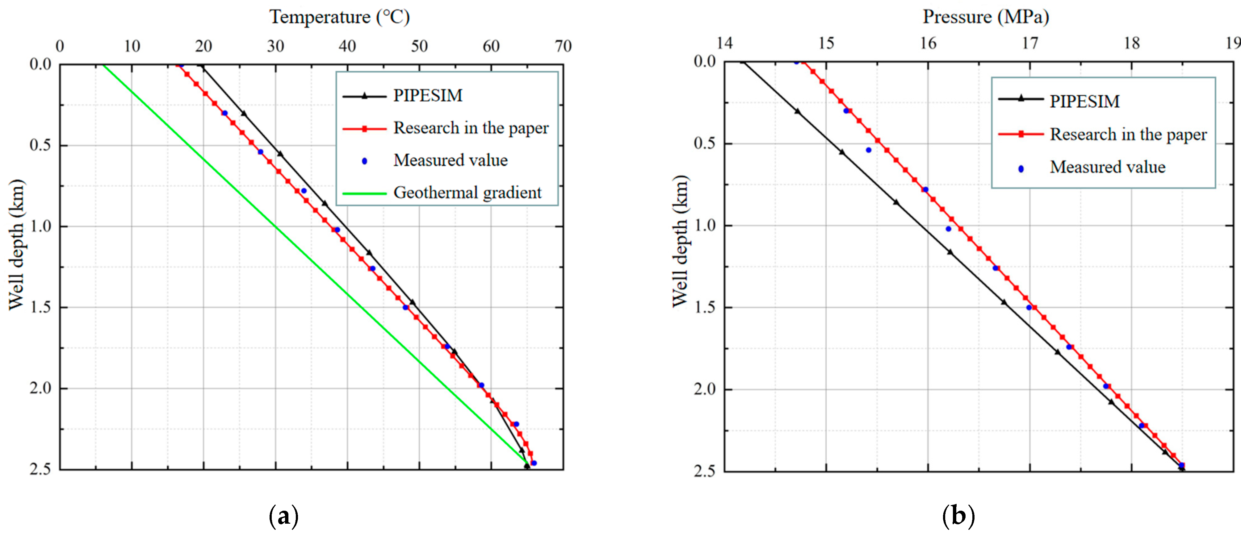
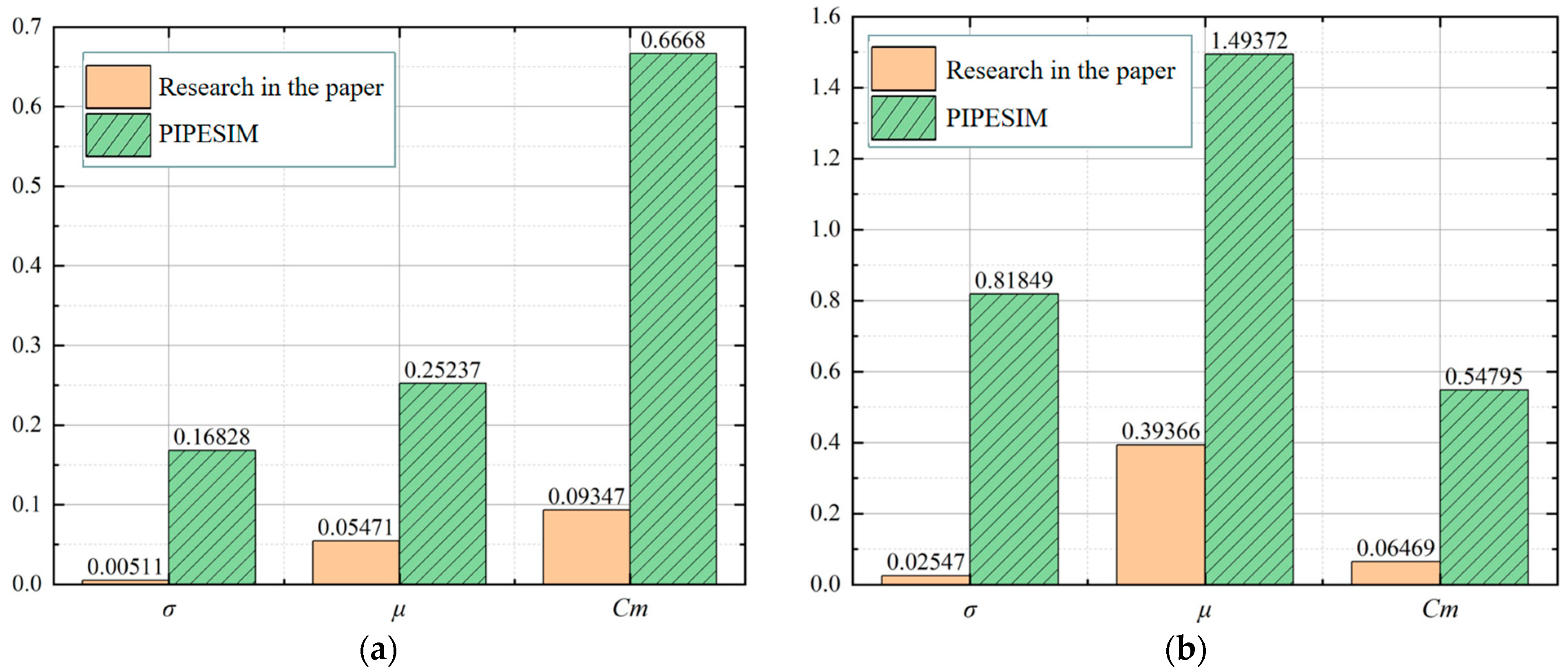
The multi-field and multi-phase coupling wellbore temperature and pressure field model were applied to wells K1 and K2, and the calculation results of this research model were analyzed and compared with the PIPESIM simulation results and measured values. We evaluated the mean μ, variance σ, and coefficient of variation C_m of the difference between the calculation results of the proposed model and those of the PIPESIM simulation results, and the measured values. The results show that the variation coefficients of the calculation results of the model proposed in this study are all less than 15%, which is more accurate than the PIPESIM simulation results.

(3)

Considering the problems of gas well liquid carrying, sand production, and gas hydrate clogging the wellbore, the design method of depth of entry of the throttle device and throttle nozzle diameter is optimized. Taking well K2 as an example and applying the downhole throttling technology, it was calculated that a throttle device with a nozzle diameter of 4 mm can be installed at a depth of 1688 m to solve the problem of hydrate formation, and at the same time, a prediction of hydrate formation can be obtained with the data of the temperature and pressure field after throttling. The results show that hydrates will not form in the wellbore of well K2 after throttling.

References

- Liu, X.K.; Liu, L.M.; Yu, Z.C.; Zhang, L.; Zhou, L.; Zhang, Z.; Guo, F. Study on the Coupling Model of Wellbore Temperature and Pressure During the Production of High Temperature and High Pressure Gas Well. Energy Rep. 2022, 8, 1249–1257. [Google Scholar] [CrossRef]
- Zheng, J.; Li, J.H.; Wu, J.; Li, Z.; Zhang, Y. Review of Downhole Throttle Failure in Oil and Gas Wells. J. Fail. Anal. Prev. 2023, 23, 609–621. [Google Scholar] [CrossRef]
- Ramecy, H. Wellbore Heat Transmission. J. Pet. Technol. 1962, 1, 427–435. [Google Scholar] [CrossRef]
- Tragesser, A.; Crawford, P.; Crawford, H. A Method for Calculating Circulating Temperatures. J. Pet. Technol. 1967, 19, 1507–1512. [Google Scholar] [CrossRef]
- Hu, Z.M. Engineering Method for Determining the Total Heat Transfer Coefficient of A Steam Injection (Hot Water) Well Shaft. Oil Drill. Prod. Technol. 1985, 1, 55–62. [Google Scholar]
- Raymond, L. Temperature Distribution in a Circulating Drilling Fluid. J. Pet. Technol. 1969, 21, 333–341. [Google Scholar] [CrossRef]
- Han, C.; Chen, W.; Ding, L.; Zhang, Q. A New Two-dimensional Transient Forecast Model of Wellbore Temperature Based on Precise Time Step Integration Method. J. Pet. Sci. Eng. 2022, 215, 110708. [Google Scholar] [CrossRef]
- Fu, Y.R.; Dou, Q.G.; Liu, W.D.; Sun, M.Q.; Sun, B.; Hu, J.P. Coupling Model for Calculating Wellbore Temperature Distribution of Thermal Insulation Tubing. Pet. Geol. Eng. 2023, 37, 103–106. [Google Scholar]
- Duns, H.; Ros NC, J. Vertical Flow of Gas and Liquid Mixtures in Wells. In Proceedings of the 6th World Petroleum Congress, Frankfurt am Main, Germany, 19 June 1963; pp. 451–465. [Google Scholar]
- Hagedorn, A.R.; Brown, K.E. Experimental Study of Pressure Gradients Occurring During Continuous Two-phase Flow in Small-diameter Vertical Conduits. J. Pet. Technol. 1965, 17, 475–484. [Google Scholar] [CrossRef]
- Bhagwat, S.M.; Chajar, A.J. A Flow Pattern Independent Drift Flux Model Based Void Fraction Correlation for a Wide Range of Gas-liquid Two Phase Flow. Int. J. Multiph. Flow 2014, 59, 186–205. [Google Scholar] [CrossRef]
- Zhang, H.; Shen, R.C.; Qimin, L. Coupling Analysis of Temperature and Pressure Distribution of Underground Gas Storage Injection-production Wellbore. Sci. Technol. Eng. 2017, 17, 66–73. [Google Scholar]
- Hasan, A.R.; Kabir, C.S.; Lin, D. Analytic Wellbore Temperature Model for Transient Gas-well Testing. SPE Reserv. Eval. Eng. 2005, 8, 240–247. [Google Scholar] [CrossRef]
- Hasan, A.R.; Kabir, C.S.; Wang, X. A Robust Steady-State Model for Flowing-fluid Temperature in Complex Wells. SPE Prod. Oper. 2009, 24, 269–276. [Google Scholar] [CrossRef]
- Xu, B.; Kabir, C.S.; Hasan, A.R. Nonisothermal reservoir/wellbore flow modeling in gas reservoirs. J. Nat. Gas Sci. Eng. 2018, 57, 89–99. [Google Scholar] [CrossRef]
- Onur, M.; Cinar, M. Modeling and Analysis of Temperature Transient Sandface and Wellbore Temperature Data from Variable Rate Well Test Data. In Proceedings of the SPE Europe Featured at 79th EAGE Conference and Exhibition, Paris, France, 12 June 2017. [Google Scholar]
- Wang, H.Y. A Non-isothermal Wellbore Model for High Pressure High Temperature Natural Gas Reservoirs and Its Application in Mitigating Wax Deposition. J. Nat. Gas Sci. Eng. 2019, 72, 103016. [Google Scholar] [CrossRef]
- Zhang, P.Y.; Wen, B.; Wang, L.J.; Haojie, L.; Min, T. Study on Wellbore Temperature Field of Shale Gas Horizontal Well Drilling in Y101 Block. Drill. Prod. Technol. 2022, 45, 1–7. [Google Scholar]
- Zheng, J.; Dou, Y.; Li, Z.; Yan, X.; Zhan, Y.; Bi, C. Investigation and Application of Wellbore Temperature and Pressure Field Coupling with Gas–liquid Two-phase Flowing. J. Pet. Explor. Prod. Technol. 2021, 12, 753–762. [Google Scholar] [CrossRef]
- Dastkhan, Y.; Kazemi, A. An Efficient Numerical Model for Nonisothermal Fluid Flow Through Porous Media. Can. J. Chem. Eng. 2021, 99, 2789–2799. [Google Scholar] [CrossRef]
- Dastkhan, Y.; Kazemi, A.; Al-Maamari, R. Well and Reservoir Characterization Using Combined Temperature and Pressure Transient Analysis: A Case Study. Results Eng. 2022, 15, 100488. [Google Scholar] [CrossRef]
- Huang, X.L.; Qi, Z.L.; Li, S.N.; Li, S.; Xiao, Q.; Mo, F.; Fang, F. Study on Prediction Model about Water Content in High Temperature and High Pressure Water Soluble Gas Reservoirs. J. Energy Resour. Technol. 2021, 143, 023501. [Google Scholar] [CrossRef]
- Jiang, D.L.; Liu, S.J.; Huang, Y.; Meng, W.; Diao, H.; Gan, B.; Zou, F. Wellbore Temperature-Pressure Coupling Model Under Deep-Water Gas Well Intervention Operation. Adv. Transdiscipl. 2022, 23, 293–305. [Google Scholar]
- Liu, J.J.; Wu, W.L.; Qian, P.; Wang, S. A Temperature-Pressure Coupling Model for Predicting Gas Temperature Profile in Gas Drilling. Therm. Sci. 2021, 25, 3493–3503. [Google Scholar] [CrossRef]
- An, J.T.; Li, J.; Huang, H.L.; Liu, G.; Chen, S.; Zhang, G. Numerical Study of Temperature Pressure Coupling Model for the Horizontal Well with a Slim Hole. Energy Sci. Eng. 2023, 11, 1060–1079. [Google Scholar] [CrossRef]
- Zhang, S.L.; Ma, F.M. Gas Downhole Throttling Technology; Petroleum Industry Press: Beijing, China, 2015; pp. 58–62. [Google Scholar]
- Huo, G.Y.; Dian, S.Y.; Xu, X. Finite Element Analysis of New Downhole Throttle Based on Orifice Value. IOP Conf. Ser. Mater. Sci. Eng. 2018, 428, 012016. [Google Scholar] [CrossRef]
- Fu, Y.; Ma, H.; Yu, C.; Dong, L.; Yang, Y.; Zhu, X.; Sun, H. Analysis of Effective Operation Performance of Wireless Control Downhole Choke. Shock. Vib. 2020, 2020, 7831819. [Google Scholar] [CrossRef]
- Furukawa, T.; Sekogchi, K. Phase Distribution for Air-Water Two Phase in Annuli. Bull. JSME 1986, 29, 3007–3014. [Google Scholar] [CrossRef]