

A Fast Workflow for Automatically Extracting the Apparent Attitude of Fractures in 3-D Digital Core Images


Abstract
:1. Introduction
2. Methodology
2.1. The Original Workflow
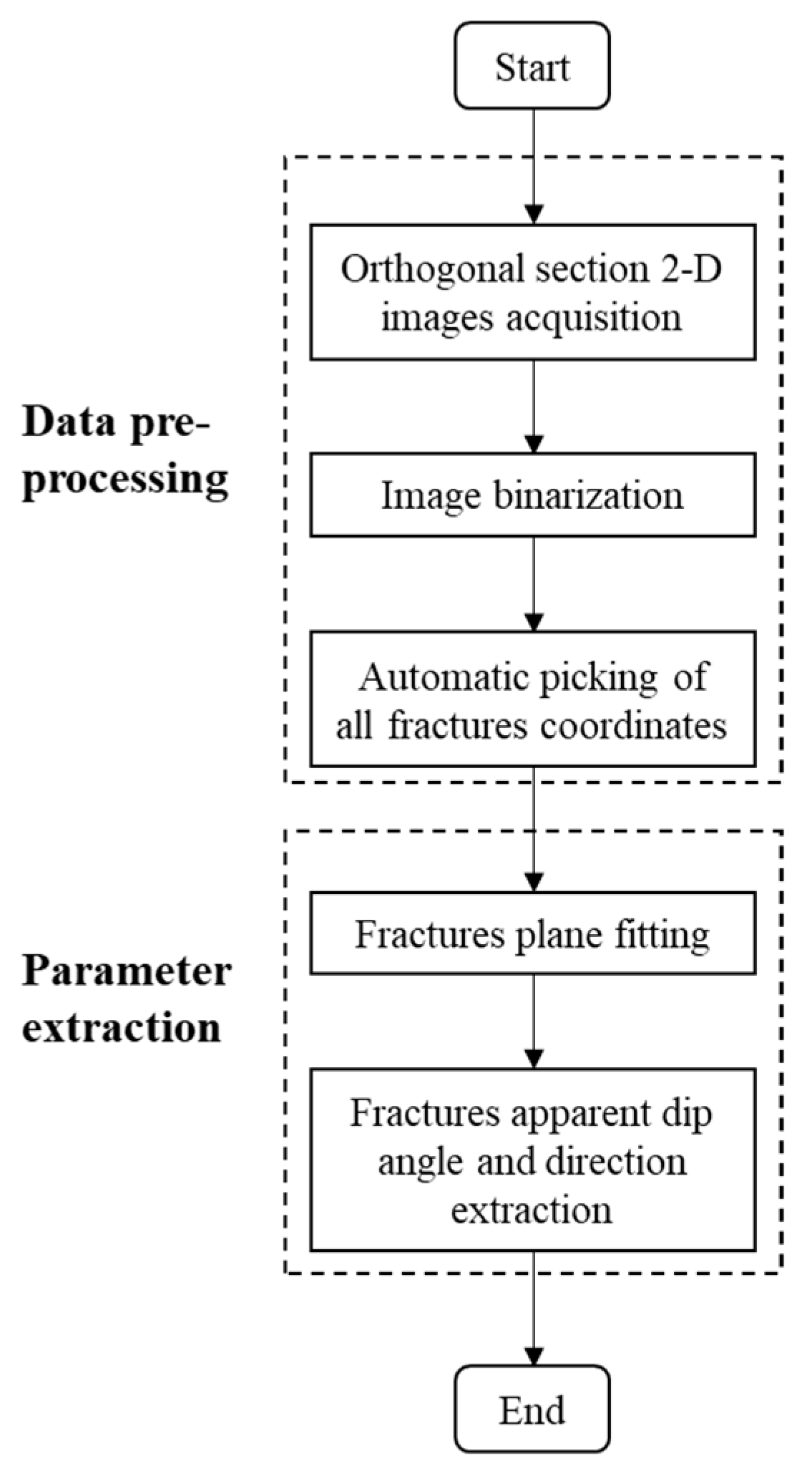
2.1.1. Data Pre-Processing in the Original Workflow
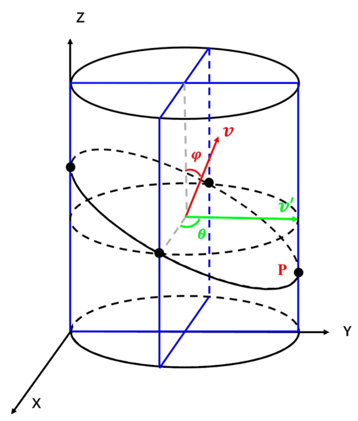
2.1.2. Extraction Method in the Original Workflow: Moments of Inertia Method
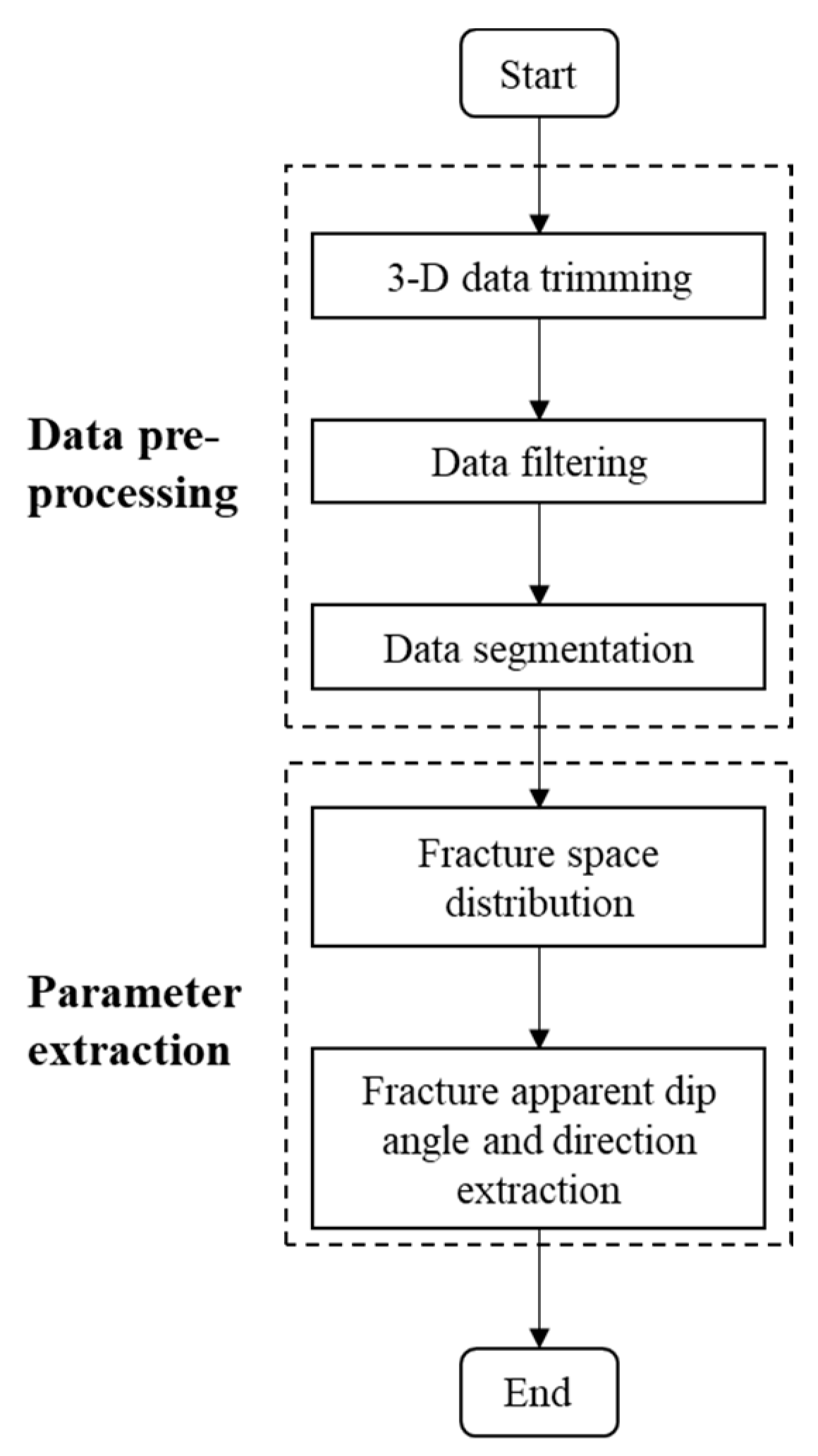
2.2. The New Workflow
2.2.1. Data Pre-Processing in the New Workflow
- Firstly, the binary image is analyzed for connected domains, specifically identifying the fracture region;
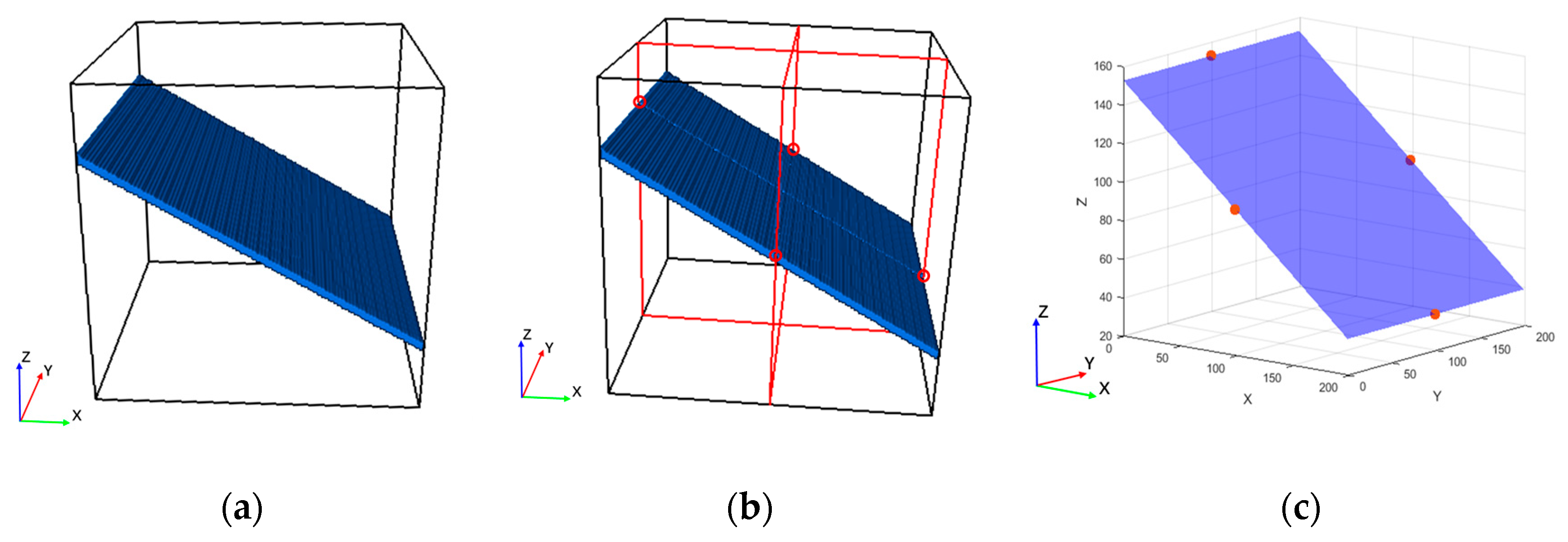
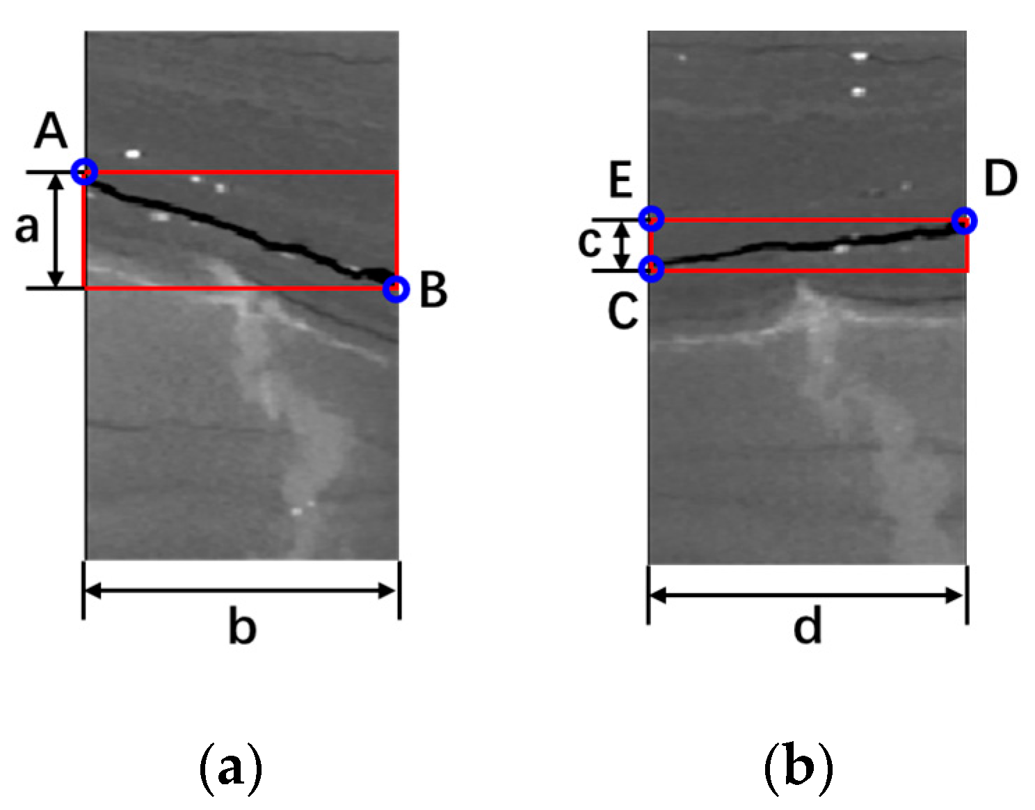
- Then, the minimum external rectangle of each connected domain is extracted. As shown in Figure 5, the coordinates of the upper left corner of the external rectangle, as well as the length and width of the rectangle, are recorded. The points A and E represent the upper left corners of the minimum external rectangles, with coordinates ( ) and (), respectively. The variables a and c represent the width of each rectangle, while b and d represent the length;
- Finally, the tilt direction of the connected domain is determined. If it is sloping downward, the coordinates for point A are (), and the coordinates for point B are () (as shown in Figure 5a). If it is sloping upward, the coordinates for point C are (), and the coordinates for point D are () (as shown in Figure 5b).
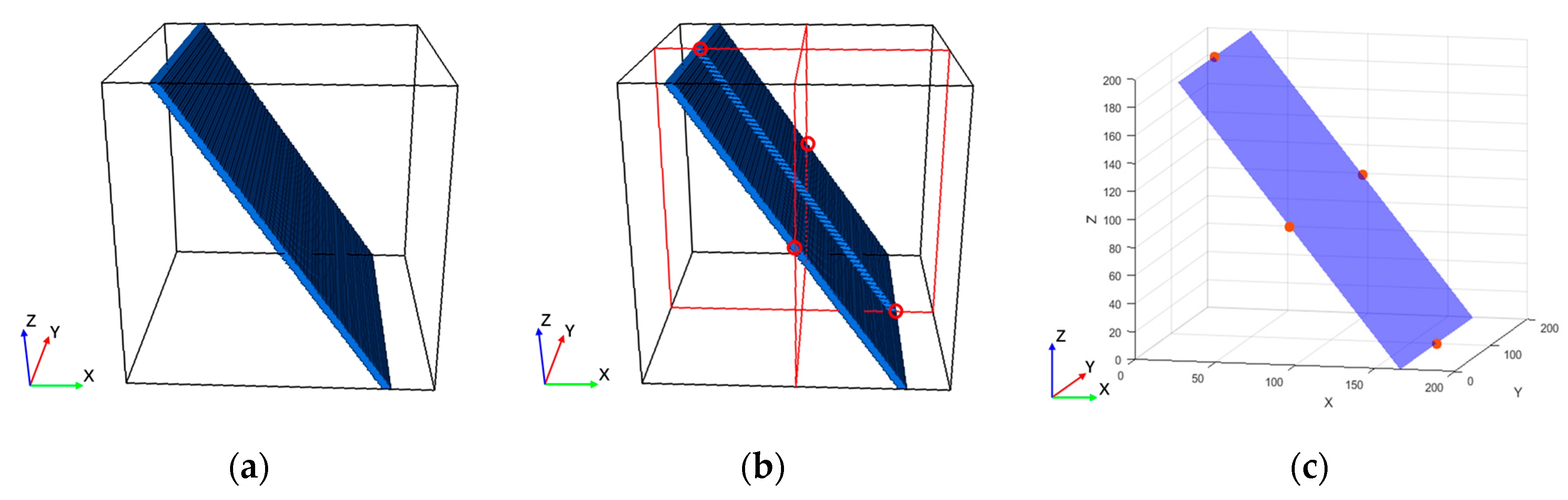
2.2.2. Extraction Method in the New Workflow: Least Squares Method
3. Application in Field Data and Results
3.1. Practical Data
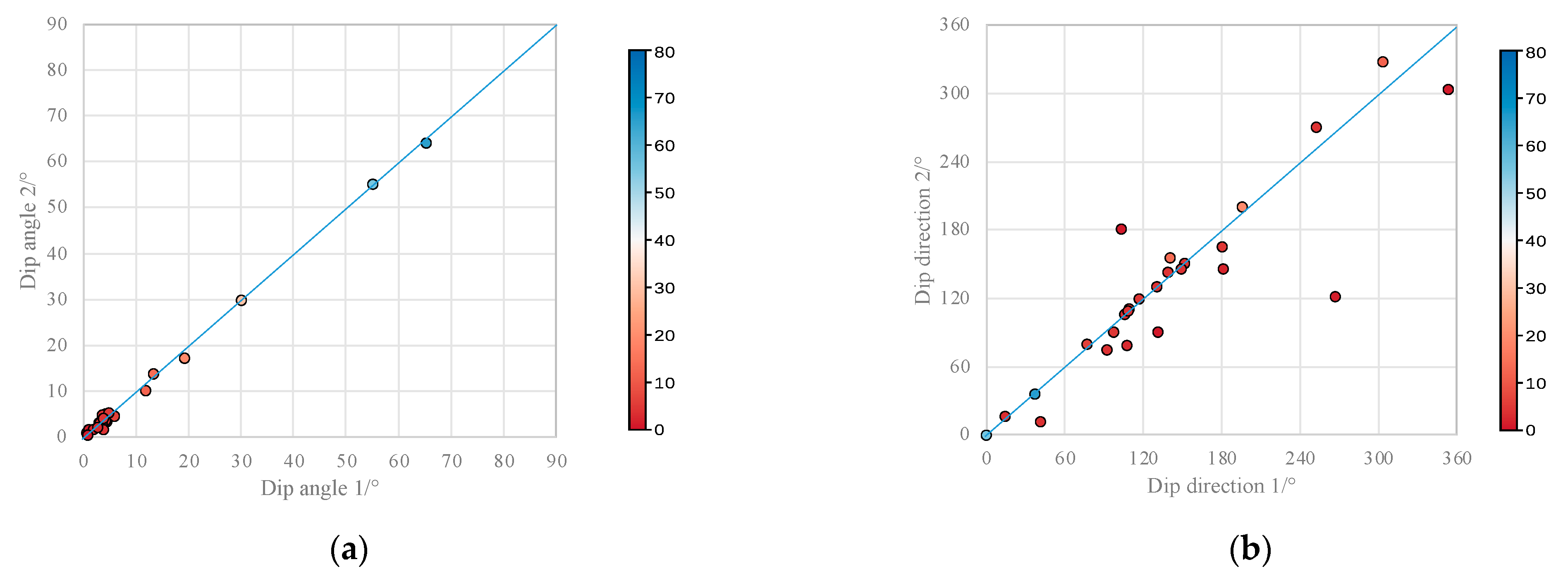
3.2. Results
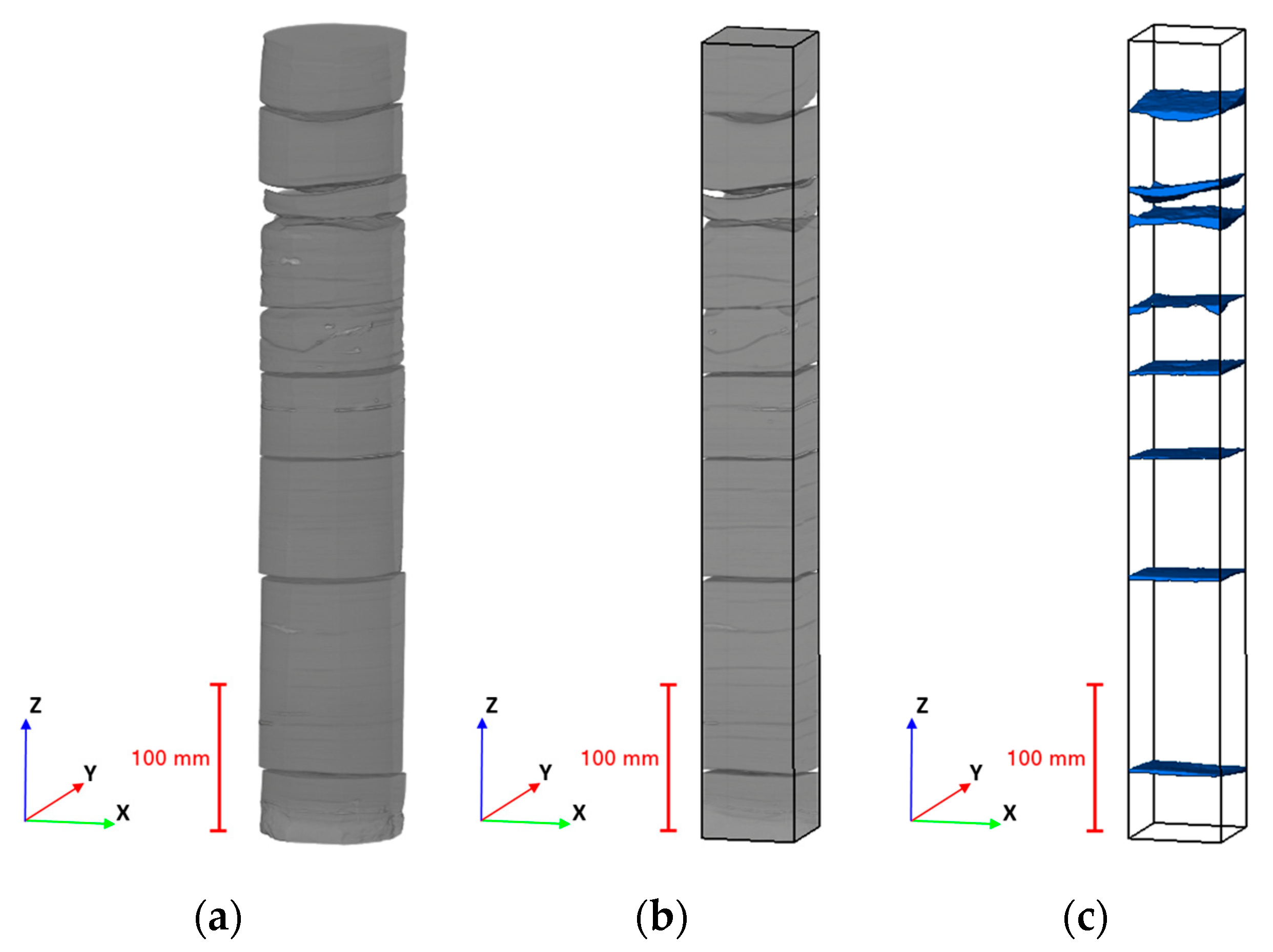
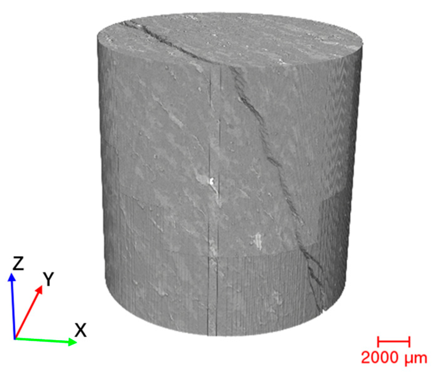
3.2.1. Micro-Fracture in Micro-CT Sample
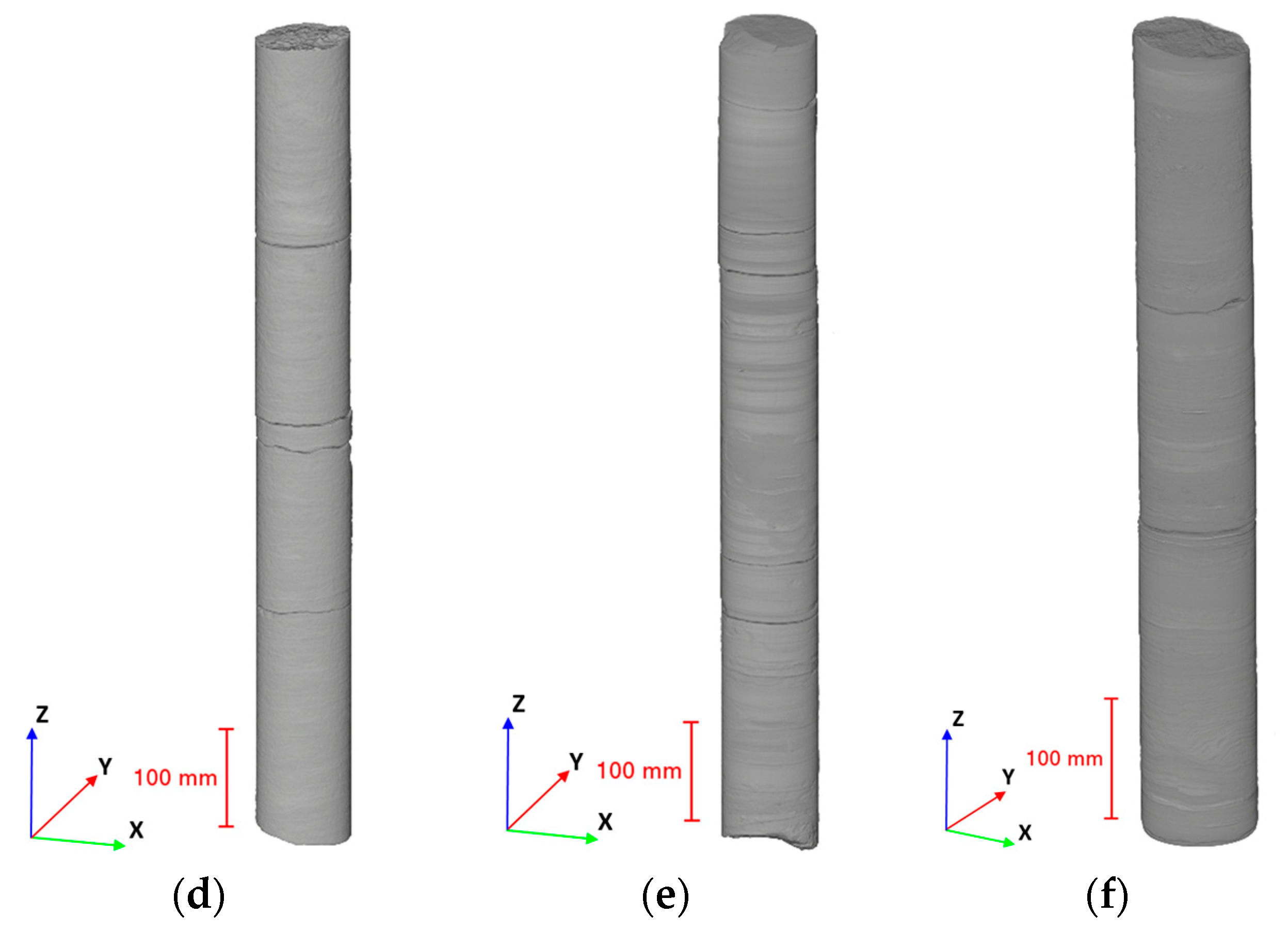
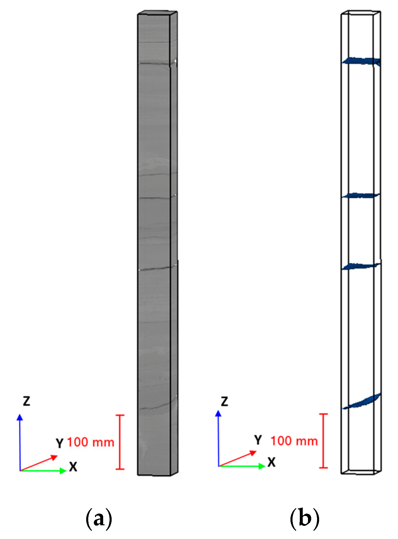
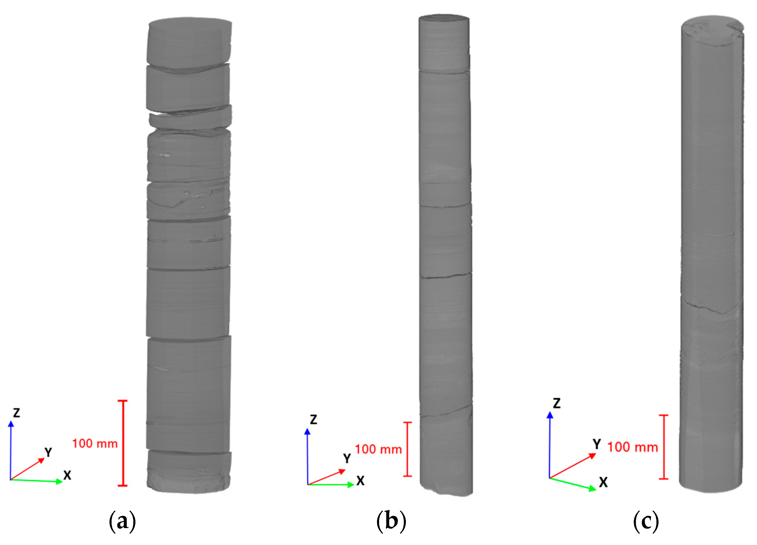
3.2.2. Macro-Fractures in Full-Hole Digital Cores
4. Discussion
5. Conclusions
Author Contributions
Funding
Data Availability Statement
Acknowledgments
Conflicts of Interest
References
- Li, C.; Zhao, L.; Liu, B.; Chen, Q.; Lu, C.; Kong, Y. Research Status, significance and Development Trend of Microfractures. Nat. Gas Geosci. 2020, 31, 402–416. [Google Scholar]
- Xiaolong, C.; Leng, T.; Yan, M.; Wang, J.; Huang, C.; Wang, Z.; Liu, Z. Study on Characteristics and Classification of Micro-Pore Structure in Tight Reservoirs for Ordos Basin. Nat. Gas Geosci. 2023, 34, 51–59. [Google Scholar]
- Li, X.; Zhang, J.; Chen, C.; Li, Z.; Liu, Z. Fracture Development Characteristics and Quantitative Prediction of Tight Reservoirs in Well Block Ma 2, Northwestern Margin, Junggar Basin. Spec. Oil Gas Reserv. 2022, 29, 50–56. [Google Scholar]
- Zou, C.; Yang, Z.; Zhu, R.; Zhang, G.; Hou, L.; Wu, S.; Tao, S.; Yuan, X.; Dong, D.; Wang, Y.; et al. Progress in China’s Unconventional Oil and Gas Exploration and Development and Theoretical Technologies. Acta Geol. Sin. 2015, 89, 979–1007. [Google Scholar]
- Yuan, J.; Cao, Y.; Li, J.; Dong, D.; Yang, R.; Li, C.; Chang, L.; Yang, J. Diversities and Disparities of Fracture Systems in the Paleogene in DN Gas Field, Kuqa Depression, Tarim Basin. Oil Gas Geol. 2017, 38, 840–850. [Google Scholar] [CrossRef]
- Lawn, B. Fracture of Brittle Solids; Cambridge University Press: Cambridge, UK, 1993; ISBN 9780521409728. [Google Scholar]
- Aydin, A. Fractures, Faults, and Hydrocarbon Entrapment, Migration and Flow. Mar. Pet. Geol. 2000, 17, 797–814. [Google Scholar] [CrossRef]
- Nelson, R.A. Geologic Analysis of Naturally Fractured Reservoirs; Gulf Professional Publishing: Houston, TX, USA, 2001. [Google Scholar]
- Schultz, R.A. Geologic Fracture Mechanics; Cambridge University Press: Cambridge, UK, 2019; ISBN 9781316996737. [Google Scholar]
- Gou, Q.; Xu, S.; Hao, F.; Yang, F.; Wang, Y.; Lu, Y.; Zhang, A.; Cheng, X.; Qing, J.; Gao, M. Study on Characterization of Micro-Fracture of Shale Based on Micro-CT. Acta Geol. Sin. 2019, 93, 2372–2382. [Google Scholar]
- Li, A.; Ding, W.; Luo, K.; Xiao, Z.K.; Wang, R.; Yin, S.; Deng, M.; He, J. Application of R/S Analysis in Fracture Identification of Shale Reservoir of the Lower Cambrian Niutitang Formation in Northern Guizhou Province, South China. Geol. J. 2020, 55, 4008–4020. [Google Scholar] [CrossRef]
- Dong, S.; Zeng, L.; Lyu, W.; Xu, C.; Liu, J.; Mao, Z.; Tian, H.; Sun, F. Fracture Identification by Semi-Supervised Learning Using Conventional Logs in Tight Sandstones of Ordos Basin, China. J. Nat. Gas Sci. Eng. 2020, 76, 103131. [Google Scholar] [CrossRef]
- Tian, M.; Li, B.; Xu, H.; Yan, D.; Gao, Y.; Lang, X. Deep Learning Assisted Well Log Inversion for Fracture Identification. Geophys. Prospect. 2021, 69, 419–433. [Google Scholar] [CrossRef]
- Zhang, S.; Yan, J.; Cai, J.; Zhu, X.; Hu, Q.; Wang, M.; Geng, B.; Zhong, G. Fracture Characteristics and Logging Identification of Lacustrine Shale in the Jiyang Depression, Bohai Bay Basin, Eastern China. Mar. Pet. Geol. 2021, 132, 105192. [Google Scholar] [CrossRef]
- Liu, X. Quantitative Analysis and Distribution Prediction of Natural Fractures in the Tight Reservoir from Jimusar Sag. Master’s Thesis, China University of Petroleum, Beijing, China, 2018. [Google Scholar]
- Du, X.; Jin, Z.; Zeng, L.; Li, S.; Liu, G.; Liang, X.; Lu, G. Development Characteristic and Controlling Factors of Natural Fractures in Chang 7 Shale Oil Reservoir, Longdong Area, Ordos Basin. Earth Sci. 2023, 48, 3045–3055. [Google Scholar] [CrossRef]
- Dong, S.; Sun, F.; He, J.; Sun, F.; Zeng, L.; Du, X. Development Characteristic and Main Controlling Factors of Fractures in Carbonate Reservoirs of Asmari Formation of A Oilfield, Iraq. J. Xi’an Shiyou Univ. Sci. Ed. 2022, 37, 34–43. [Google Scholar]
- Lu, Q. Fracture Development Characteristics and Distribution Law of Carbonate Reservoir in the Buried Hill of Nanpu Depression. Master’s Thesis, Northeast Petroleum University, Daqing, China, 2022. [Google Scholar]
- Hu, H.; Ju, W.; Guo, W.; Ning, W.; Liang, Y.; Yu, G. Development Characteristics and Prediction of Natural Fractures within Shale Gas Reservois, Haiba Block of Southern Sichuan Basin. Unconv. Oil Gas 2023, 10, 61–68. [Google Scholar]
- Mazdarani, A.; Kadkhodaie, A.; Wood, D.A.; Soluki, Z. Natural Fractures Characterization by Integration of FMI Logs, Well Logs and Core Data: A Case Study from the Sarvak Formation (Iran). J. Pet. Explor. Prod. Technol. 2023, 13, 1247–1263. [Google Scholar] [CrossRef]
- Li, L.; Sang, X.; Chen, X. Research and Progress on Fracture of Low-Permeability Reservoir. Prog. Geophys. 2017, 32, 2472–2484. [Google Scholar]
- Li, W.; Lin, T.; Wang, A. Research Progress of Fractures in Tight Sandstone Gas Reservoirs. Oil Gas Prod. 2021, 49, 25–29. [Google Scholar]
- Lü, W.; Zeng, L.; Liu, J.; Wang, C.; Zhu, J. Fracture Research Progress in Low Permeability Tight Rservoirs. Geol. Sci. Technol. Inf. 2016, 35, 74–83. [Google Scholar]
- Schwartz, B.C. Fracture Pattern Characterization of the Tensleep Formation, Teapot Dome, Wyoming. Master’s Thesis, West Virginia University, Morgantown, WV, USA, 2006. [Google Scholar]
- Shafiabadi, M.; Kamkar-Rouhani, A.; Sajadi, S.M. Identification of the Fractures of Carbonate Reservoirs and Determination of Their Dips from FMI Image Logs Using Hough Transform Algorithm. Oil Gas Sci. Technol. 2021, 76, 37. [Google Scholar] [CrossRef]
- Arif, M.; Mahmoud, M.; Zhang, Y.; Iglauer, S. X-Ray Tomography Imaging of Shale Microstructures: A Review in the Context of Multiscale Correlative Imaging. Int. J. Coal Geol. 2021, 233, 103641. [Google Scholar] [CrossRef]
- Nie, X.; Li, B.; Zhang, J.; Zhang, C.; Zhang, Z. Numerical Simulation of Electrical Properties of Fractured Carbonate Reservoirs Based on Digital Cores. J. Yangtze Univ. Nat. Sci. Ed. 2022, 19, 20–29. [Google Scholar] [CrossRef]
- Qin, Y. A Study on Micro Pore Structure and Pore-Throat Connectivity in Tight Sandstone Reservoir: A Case of the Chang 7 Reservoir in Ordos Basin. Master’s Thesis, Nanjing University, Nanjing, China, 2021. [Google Scholar]
- Borrelli, M.; Campilongo, G.; Critelli, S.; Perrotta Ida, D.; Perri, E. 3D Nanopores Modeling Using TEM-Tomography (Dolostones—Upper Triassic). Mar. Pet. Geol. 2019, 99, 443–452. [Google Scholar] [CrossRef]
- Zhao, S.; Li, Y.; Wang, Y.; Ma, Z.; Huang, X. Quantitative Study on Coal and Shale Pore Structure and Surface Roughness Based on Atomic Force Microscopy and Image Processing. Fuel 2019, 244, 78–90. [Google Scholar] [CrossRef]
- Ramandi, H.L.; Mostaghimi, P.; Armstrong, R.T. Digital Rock Analysis for Accurate Prediction of Fractured Media Permeability. J. Hydrol. 2017, 554, 817–826. [Google Scholar] [CrossRef]
- Garum, M.; Glover, P.W.J.; Lorinczi, P.; Drummond-Brydson, R.; Hassanpour, A. Micro- And Nano-Scale Pore Structure in Gas Shale Using Xμ-CT and FIB-SEM Techniques. Energy Fuels 2020, 34, 12340–12353. [Google Scholar] [CrossRef]
- Zhang, W.; Wang, J. Characterization of Microscopic Pore Structure of Different Coal Types Based on Micro CT. Coal Sci. Technol. 2021, 49, 85–92. [Google Scholar]
- Li, B.; Nie, X.; Cai, J.; Zhou, X.; Wang, C.; Han, D. U-Net Model for Multi-Component Digital Rock Modeling of Shales Based on CT and QEMSCAN Images. J. Pet. Sci. Eng. 2022, 216, 110734. [Google Scholar] [CrossRef]
- Li, X.; Li, B.; Liu, F.; Li, T.; Nie, X. Advances in the Application of Deep Learning Methods to Digital Rock Technology. Adv. Geo-Energy Res. 2023, 8, 5–18. [Google Scholar] [CrossRef]
- Kelly, S.; El-Sobky, H.; Torres-Verdín, C.; Balhoff, M.T. Assessing the Utility of FIB-SEM Images for Shale Digital Rock Physics. Adv. Water Resour. 2016, 95, 302–316. [Google Scholar] [CrossRef]
- Wang, P.; Zhang, C.; Li, X.; Zhang, K.; Yuan, Y.; Zang, X.; Cui, W.; Liu, S.; Jiang, Z. Organic Matter Pores Structure and Evolution in Shales Based on the He Ion Microscopy (HIM): A Case Study from the Triassic Yanchang, Lower Silurian Longmaxi and Lower Cambrian Niutitang Shales in China. J. Nat. Gas Sci. Eng. 2020, 84, 103682. [Google Scholar] [CrossRef]
- Li, Y.; Yang, J.; Pan, Z.; Tong, W. Nanoscale Pore Structure and Mechanical Property Analysis of Coal: An Insight Combining AFM and SEM Images. Fuel 2020, 260, 116352. [Google Scholar] [CrossRef]
- Liu, D.; Zhao, Z.; Cai, Y.; Sun, F.; Zhou, Y. Review on Applications of X-Ray Computed Tomography for Coal Characterization: Recent Progress and Perspectives. Energy Fuels 2022, 36, 6659–6674. [Google Scholar] [CrossRef]
- Wang, Z.; Sun, W.; Shui, Y.; Liu, P. Computed Tomography Observation and Image-Based Simulation of Fracture Propagation in Compressed Coal. Energies 2023, 16, 260. [Google Scholar] [CrossRef]
- Li, Y.; He, S.; Deng, X.; Xu, Y. Characterization of Macropore Structure of Malan Loess in NW China Based on 3D Pipe Models Constructed by Using Computed Tomography Technology. J. Asian Earth Sci. 2018, 154, 271–279. [Google Scholar] [CrossRef]
- Li, X.; Lu, Y.; Zhang, X.; Fan, W.; Lu, Y.; Pan, W. Quantification of Macropores of Malan Loess and the Hydraulic Significance on Slope Stability by X-Ray Computed Tomography. Environ. Earth Sci. 2019, 78, 522. [Google Scholar] [CrossRef]
- Yang, B.; Wang, H.; Wang, B.; Shen, Z.; Zheng, Y.; Jia, Z.; Yan, W. Digital Quantification of Fracture in Full-Scale Rock Using Micro-CT Images: A Fracturing Experiment with N2 and CO2. J. Pet. Sci. Eng. 2021, 196, 107682. [Google Scholar] [CrossRef]
- Iassonov, P.; Gebrenegus, T.; Tuller, M. Segmentation of X-Ray Computed Tomography Images of Porous Materials: A Crucial Step for Characterization and Quantitative Analysis of Pore Structures. Water Resour. Res. 2009, 45, 1–12. [Google Scholar] [CrossRef]
- Tuller, M.; Kulkarni, R.; Fink, W. Segmentation of X-Ray CT Data of Porous Materials: A Review of Global and Locally Adaptive Algorithms. Soil- Water- Root Process. Adv. Tomogr. Imaging 2015, 61, 157–182. [Google Scholar] [CrossRef]
- Nie, X.; Zou, C.; Xiao, K.; Xu, J.; Niu, Y.; Kong, G. Core Spatial Position Restoring of WFSD-1 Borehole with Borehole Imaging Logging Data. Prog. Geophys. 2012, 27, 0075–0082. [Google Scholar]
- Nie, X.; Zou, C.; Pan, L.; Huang, Z.; Liu, D. Fracture Analysis and Determination of In-Situ Stress Direction from Resistivity and Acoustic Image Logs and Core Data in the Wenchuan Earthquake Fault Scientific Drilling Borehole-2 (50–1370 m). Tectonophysics 2013, 593, 161–171. [Google Scholar] [CrossRef]


| Sample | Voxel Size | Resolution |
|---|---|---|
| 1 | 800 × 800 × 800 | 19.96 μm |
| 2 | 140 × 140 × 1110 | 0.468 mm |
| 3 | 130 × 130 × 1720 | 0.468 mm |
| 4 | 140 × 140 × 1500 | 0.468 mm |
| 5 | 140 × 140 × 1710 | 0.468 mm |
| 6 | 140 × 140 × 1670 | 0.468 mm |
| 7 | 140 × 140 × 1380 | 0.468 mm |
| Sample | Fracture | Dip Angle 1 (°) | Dip Angle 2 (°) | Absolute Error | Relative Error | Dip Direction 1 (°) | Dip Direction 2 (°) | Absolute Error 2 | Relative Error 2 |
|---|---|---|---|---|---|---|---|---|---|
| 1 | 1 | 65.28 | 64.14 | 1.14 | 1.74% | 37.11 | 35.73 | 1.38 | 3.71% |
| 2 | 1 | 1.16 | 1.30 | 0.15 | 12.55% | 266.95 | 121.06 | 145.88 | 54.65% |
| 2 | 13.41 | 13.76 | 0.35 | 2.58% | 140.68 | 155.77 | −15.09 | −10.73% | |
| 3 | 0.69 | 0.84 | 0.14 | 20.81% | 131.01 | 90.81 | 40.20 | 30.69% | |
| 4 | 4.05 | 4.24 | 0.19 | 4.67% | 151.87 | 150.95 | 0.93 | 0.61% | |
| 5 | 4.09 | 4.12 | 0.03 | 0.64% | 139.27 | 143.12 | −3.85 | −2.77% | |
| 6 | 4.45 | 3.32 | 1.13 | 25.41% | 116.70 | 119.73 | −3.04 | −2.60% | |
| 7 | 4.32 | 3.52 | 0.80 | 18.59% | 109.31 | 110.51 | −1.21 | −1.10% | |
| 8 | 6.00 | 4.60 | 1.40 | 23.33% | 76.89 | 79.72 | −2.83 | −3.68% | |
| 3 | 1 | 1.02 | 1.58 | 0.57 | 55.81% | 353.27 | 303.74 | 49.54 | 14.02% |
| 2 | 1.92 | 1.58 | 0.35 | 18.00% | 181.02 | 146.23 | 34.79 | 19.22% | |
| 3 | 4.27 | 4.97 | 0.70 | 16.33% | 180.56 | 164.80 | 15.76 | 8.73% | |
| 4 | 19.33 | 17.18 | 2.15 | 11.13% | 195.77 | 200.21 | −4.44 | −2.27% | |
| 4 | 1 | 11.92 | 10.10 | 1.82 | 15.30% | 303.36 | 328.21 | −24.86 | −8.19% |
| 5 | 1 | 3.64 | 3.22 | 0.42 | 11.52% | 130.64 | 129.81 | 0.83 | 0.64% |
| 2 | 3.65 | 2.98 | 0.67 | 18.39% | 148.98 | 146.26 | 2.71 | 1.82% | |
| 3 | 3.33 | 2.11 | 1.22 | 36.75% | 41.57 | 11.12 | 30.45 | 73.24% | |
| 4 | 3.64 | 4.69 | 1.06 | 29.07% | 92.63 | 74.83 | 17.80 | 19.22% | |
| 6 | 1 | 3.05 | 2.99 | 0.06 | 1.97% | 14.57 | 16.12 | −1.55 | −10.67% |
| 2 | 3.27 | 3.00 | 0.27 | 8.26% | 106.07 | 105.96 | 0.10 | 0.10% | |
| 3 | 4.77 | 5.34 | 0.57 | 12.01% | 97.69 | 90.01 | 7.68 | 7.86% | |
| 4 | 0.89 | 0.41 | 0.48 | 54.11% | 103.57 | 180.63 | −77.06 | −74.40% | |
| 5 | 3.89 | 3.91 | 0.02 | 0.39% | 108.14 | 108.46 | −0.32 | −0.30% | |
| 7 | 1 | 3.77 | 1.66 | 2.12 | 56.08% | 252.82 | 270.31 | −17.49 | −6.92% |
| 2 | 2.76 | 2.09 | 0.67 | 24.21% | 107.73 | 78.40 | 29.33 | 27.22% |
Disclaimer/Publisher’s Note: The statements, opinions and data contained in all publications are solely those of the individual author(s) and contributor(s) and not of MDPI and/or the editor(s). MDPI and/or the editor(s) disclaim responsibility for any injury to people or property resulting from any ideas, methods, instructions or products referred to in the content. |
© 2023 by the authors. Licensee MDPI, Basel, Switzerland. This article is an open access article distributed under the terms and conditions of the Creative Commons Attribution (CC BY) license (https://creativecommons.org/licenses/by/4.0/).
Share and Cite
Zhou, Y.; Chang, D.; Zheng, J.; Zhu, D.; Nie, X. A Fast Workflow for Automatically Extracting the Apparent Attitude of Fractures in 3-D Digital Core Images. Processes 2023, 11, 2517. https://doi.org/10.3390/pr11092517
Zhou Y, Chang D, Zheng J, Zhu D, Nie X. A Fast Workflow for Automatically Extracting the Apparent Attitude of Fractures in 3-D Digital Core Images. Processes. 2023; 11(9):2517. https://doi.org/10.3390/pr11092517
Chicago/Turabian StyleZhou, Ying, Deshuang Chang, Jianxiong Zheng, Douxing Zhu, and Xin Nie. 2023. "A Fast Workflow for Automatically Extracting the Apparent Attitude of Fractures in 3-D Digital Core Images" Processes 11, no. 9: 2517. https://doi.org/10.3390/pr11092517
APA StyleZhou, Y., Chang, D., Zheng, J., Zhu, D., & Nie, X. (2023). A Fast Workflow for Automatically Extracting the Apparent Attitude of Fractures in 3-D Digital Core Images. Processes, 11(9), 2517. https://doi.org/10.3390/pr11092517