Estimating APC Model Parameters for Dynamic Intervals Determined Using Change-Point Detection in Continuous Processes in the Petrochemical Industry

Abstract

Several papers have proven that advanced process controller (APC) systems can save more energy in the process than proportional-integral-differential (PID) controller systems. Therefore, implementing an APC system is ultimately beneficial for saving energy in the plant. In a typical APC system deployment, the APC model parameters are calculated from dynamic data intervals obtained through the plant test. However, depending on the proficiency of the APC engineer, the results of the plant test and the APC model parameters are implemented differently. To minimize the influence of the APC engineer and calculate universal APC model parameters, a technique is needed to obtain dynamic data without a plant test. In this study, we utilize time-series data from a real petrochemical plant to determine dynamic intervals and estimate APC model parameters, which have not been investigated in previous studies. This involves extracting the data of the dynamic intervals with the smallest mean absolute error (MAE) by utilizing statistical techniques such as pruned exact linear time, linear kernel, and radial basis function kernel of change-point detection (CPD). After that, we fix the hyper parameters at the minimum MAE value and estimate the APC model parameters by training with the data from the dynamic intervals. The estimated APC model parameters are applied to the APC program to compare the APC model fitting rate and verify the accuracy of the APC model parameters in the dynamic intervals obtained through CPD. The final validation of the model fitting rates demonstrates that the identification of the dynamic intervals and the estimation of the APC model parameters through CPD show high accuracy. We show that it is possible to estimate APC model parameters from dynamic intervals determined by CPD without a plant test.

1. Introduction

Most petrochemical plants use a proportional-integral-differential (PID) controller system for feedback control [1]. However, a PID system is gradually being expanded and introduced into an advanced process controller (APC), which is an integrated feedforward and feedback control system that predicts external influences.

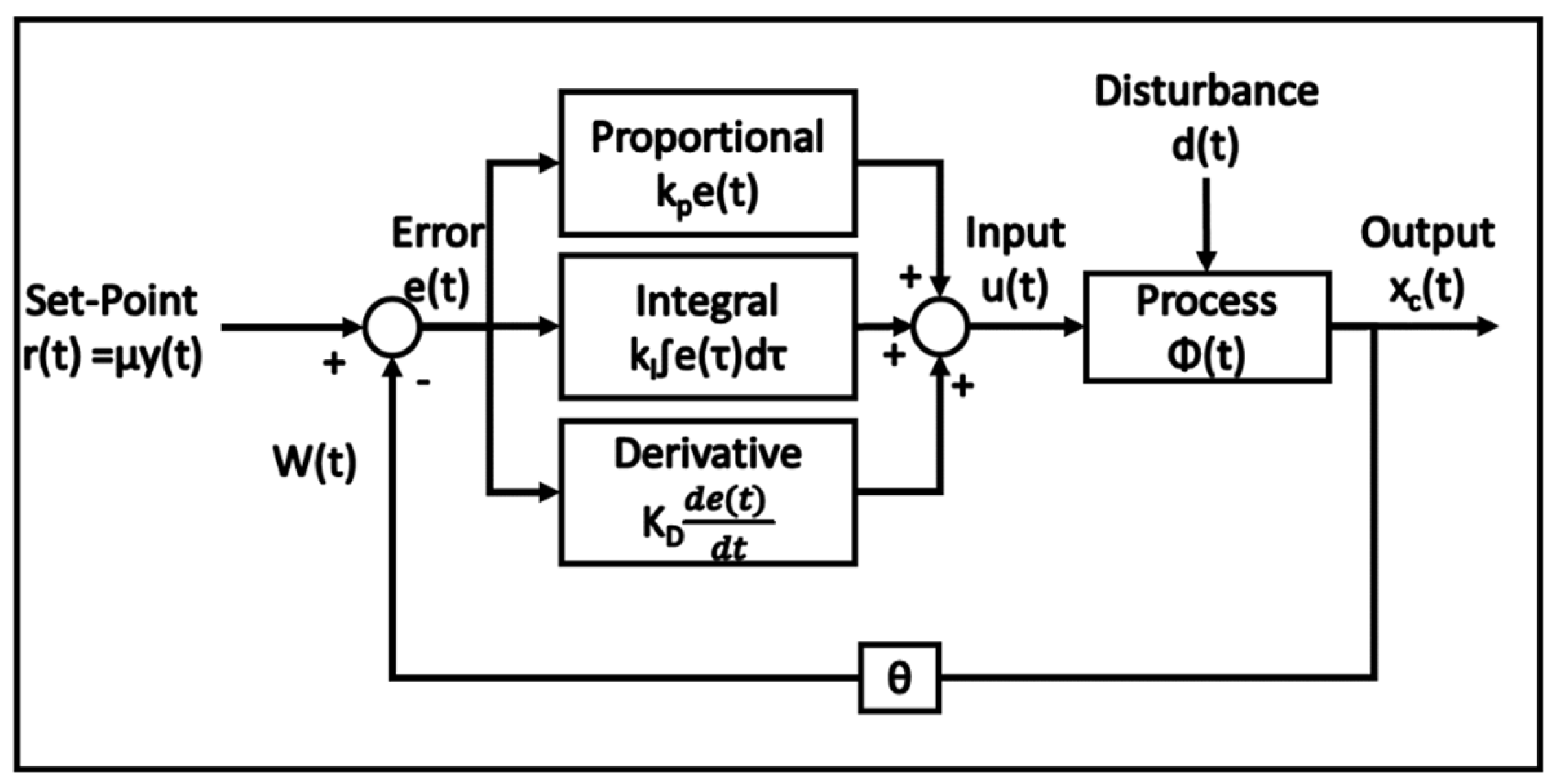
The representative control method of classical control theory is PID control [2,3]. As shown in Figure 1, the transfer function of the PID controller is composed of three terms: proportional, integral, and derivative. $K_P$, $K_I$, and $K_D$ are the proportional, integral, and differential gains, respectively. The overshoot increases with $K_P$, but the rise time decreases, approaching the target value faster and reducing the steady-state error. However, this requires considerable control, which can strain the system. The settling time is unaffected. As $K_I$ increases, the overshoot increases owing to the large change in the amount of control over the residual deviation from the steady state. Since the output changes are gradual, the rise time decreases slightly, the settling time increases, and the steady-state error, which is the goal of integral control, is eliminated. Increasing $K_D$ reduces the overshoot, rise time, and settling time because the error is corrected rapidly. However, the steady-state error remains unaffected. The Laplace inversion of the transfer function $G_{PID}$(s) given by Equation (1) yields the output equation in the time domain, as shown in Equation (2).

$$G_{PID}\left(\mathrm{s}\right)=K_P+\frac{K_I}{s}+K_{D}s$$

(1)

$$\mathrm{y}\left(\mathrm{t}\right)=K_{P}e\left(t\right)+K_I{\int }_0^{t}e\left(\tau \right) d\tau +K_D\frac{de\left(t\right)}{dt}$$

(2)

Figure 1. PID system structure.

PID systems are characterized by 1:1 control between the process variable and the manipulative variable. Additionally, it is a feedback control system that compensates for the difference between predicted and actual values in real time. The control performance is determined by the PID tuning value.

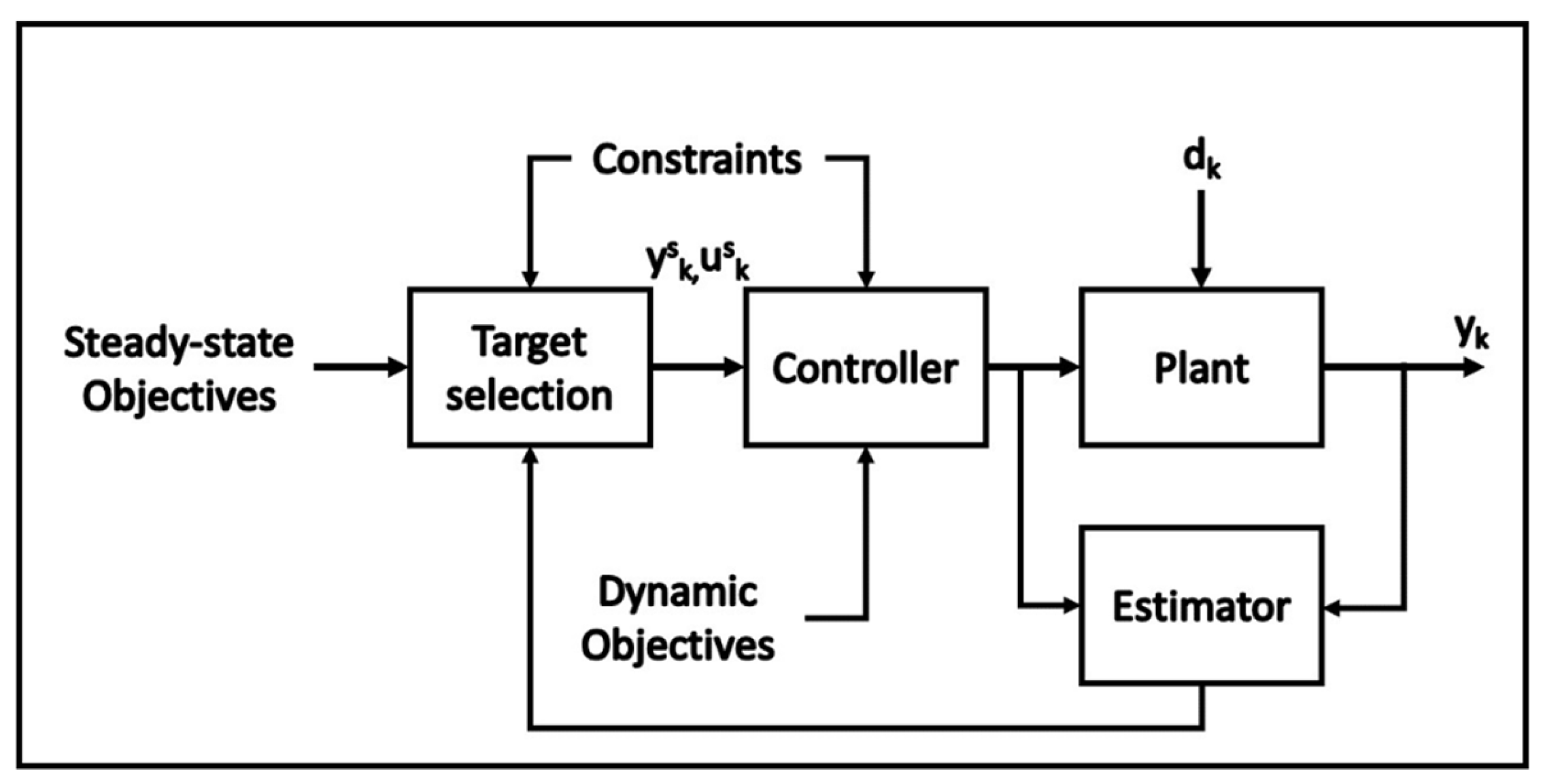
Unlike PID systems, APC systems can be applied to processes with long time delays, unstable processes, and multi-variable processes. APC control is characterized by the N:N control method, which controls multiple process variables with multiple manipulative variables; the mixed feedback control method, which controls by compensating for the difference between the predicted and actual value in real time; and the feedforward control method, which considers the influence of external disturbance variables in advance and controls before the external influence [4]. Figure 2 shows a schematic of an APC system.

Figure 2. Structure of an APC system.

In general, an APC system used in industrial applications is modeled as a first-order time-delay control system, as shown in Equation (3), where K = gain, D = delay, τ = time constant, t = elapsed time, x = manipulative variable, and y = process variable [5]. Through a Laplace inverse transformation, the output equation can be obtained in the time domain of the first-order time-delay model, as shown by Equation (4).

$${\mathrm{G}}_{\mathrm{M}}\left(\mathrm{s}\right)=\mathrm{K}\frac{{\mathrm{e}}^{-\mathrm{D}\mathrm{s}}}{1+\mathsf{\tau }\mathrm{s}}$$

(3)

$$\mathrm{y}\left(\mathrm{t}\right)=\mathrm{K}\left(1-{\mathrm{e}}^{-\frac{\mathrm{t}}{\mathsf{\tau }}}\right)·\mathrm{x}\left(\mathrm{t}-\mathrm{D}\right)$$

(4)

A typical APC system consists of a system model, constraints, disturbance model, cost function, optimization method, and control range, all of which can affect the performance of the APC system [6,7,8,9,10]. Previous papers have demonstrated that APC systems can save energy over PID systems, so replacing a PID system with an APC system can ultimately save energy in a plant [11,12,13,14,15]. APC model parameter estimates for a typical APC system can be obtained from dynamic data spheres obtained from plant tests. The performance of the APC system is determined by the APC model parameter values. The APC systems require regular updates of the APC model parameters over time due to changes in the plant’s production grade, equipment obsolescence and replacement, etc. Programs (MATLAB, Model-ID, etc.) that help APC engineers easily obtain model parameters are being commercialized, but in the process of conducting on-site plant tests and calculating APC model parameters, a problem occurs where the results of plant tests and APC model parameters are implemented differently depending on the proficiency of APC engineers. Therefore, to minimize the influence of APC engineer proficiency and calculate universal APC model parameters, a technique is needed to obtain dynamic interval data without a plant test process.

To estimate APC model parameters, we need to know the correlation between process variables (PVs) and manipulative variables (MVs) in the data of dynamic intervals. Here, DVs refer to disturbance variables, which are non-manipulable variables that come from outside the actual process, but for the purpose of the study, which is to estimate APC model parameters, they are the same as the MVs, which are manipulative variables. However, it is often difficult to determine the dynamic intervals because of the complexity of process dynamics [16]. In this study, we used time-series data from a real petrochemical plant to extract the dynamic intervals of the time-series data using various statistical techniques for change-point detection (CPD) [17]. To estimate the APC model parameters accurately, pruned exact linear time (PELT)-based, linear kernel-based, and radial basis function (RBF) kernel-based learning of CPD were compared to determine the hyper parameter of the dynamic intervals with the smallest mean absolute error (MAE) [18]. The APC model parameters were then estimated using the Levenberg–Marquardt algorithm in the dynamic range of the fixed hyperparameter. It involves applying the estimated APC model parameters to the APC program to compare the fitting rate in three intervals of randomized evaluation data to verify the accuracy of the APC model parameters in the dynamic intervals obtained through CPD.

By comparing the estimated APC model parameters with the fitting rate in three random intervals of the evaluation data, we found that the average fitting rates of 86.09% and 79.94% were obtained for Plants A and B, respectively. Through the final verification of the fitting rates, it was confirmed that the identification of dynamic intervals and the estimation of APC model parameters through CPD were highly significant. This demonstrates that APC model parameters can be estimated from dynamic intervals identified through CPD without the need for plant testing, which requires engineers to manipulate them arbitrarily and manually. Various prior studies have confirmed that the data identification of dynamic intervals through CPD is quite accurate [19,20,21,22]. However, no study has been conducted to estimate APC model parameters from dynamic intervals of data identified by CPD. In this study, we identify dynamic intervals through CPD in time-series data in the petrochemical process industry. Then, we estimate the APC model parameters within the data of the dynamic intervals, and finally, we verify the accuracy of the dynamic intervals and the APC model parameters. The final model fitting rate verification proves the achievement of this study.

2. Background and Methodology

2.1. APC Model Design Flow

Considering the inherent characteristics of the process, such as time delay, mutual interference, back reaction, and process constraints, the APC system was introduced because PID operation alone has limitations in performing optimized operation. The following steps are necessary to carry out an APC project:

(1)

Functional Design

By analyzing the flow of the target process and the user’s operational purpose, the PID loop performance of the MV used by the APC is determined, and the control strategy, such as the PV, MV, and DV, is set for optimal operation. During the pre-process test period, the performance of each instrument must be understood to prevent schedule delays.

(2)

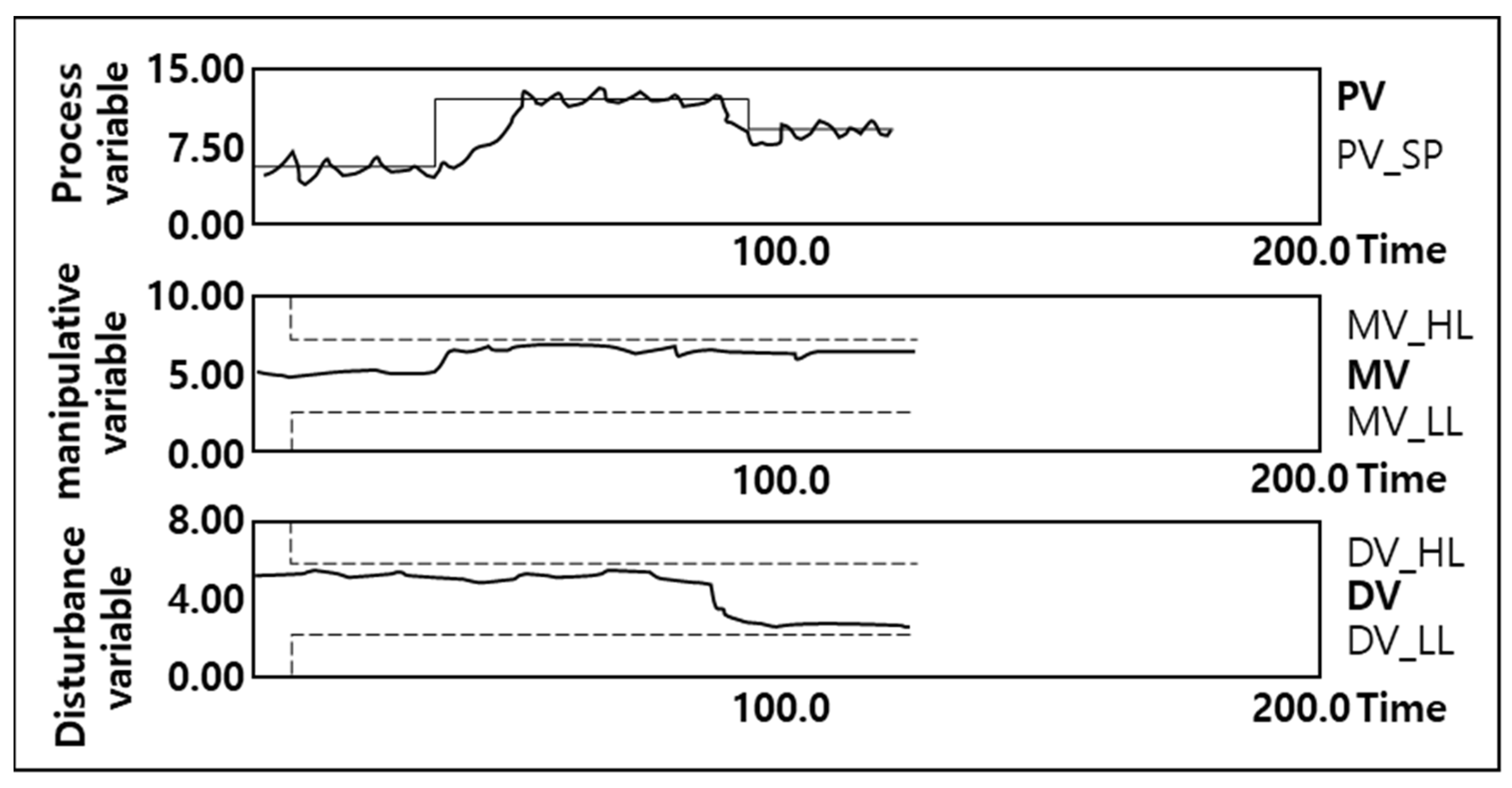
Plant Test

This is the process of developing a model of the APC controller to apply to the actual APC. To develop the model, a plant test is conducted to monitor the movement of the PV by changing the expected MV and DV with the desired amplitude for an appropriate period. Since the actual process is moved arbitrarily, during the plant test, sufficient training of operators must be provided, sufficient consultations with the production team must be conducted, and care is needed to prevent process problems. Figure 3 shows an example of a plant test.

Figure 3. Plant test.

(3)

Detail Design

In detailed design, plant test data are used to finalize the process variables selected in functional design. In addition, a dynamic process model is built between the finalized variables. Before applying the constructed dynamic process model to the actual field APC system, an offline test is performed to verify the control structure and performance in a virtual simulation environment. Through the offline test, it can be verified that the PV is properly controlled by the MV and DV according to the change in the PV’s set point. The dynamic process model of the PV is designed using an APC simulator, which is available from most APC vendors, as shown in Figure 4. After validating the dynamic process model through the APC simulator, it can be built online into the actual field APC system to reduce the implementation error of the APC system (Figure 5).

Figure 4. Calculation of the dynamic characteristic model of the APC.

Figure 5. Offline validation of the APC system.

(4)

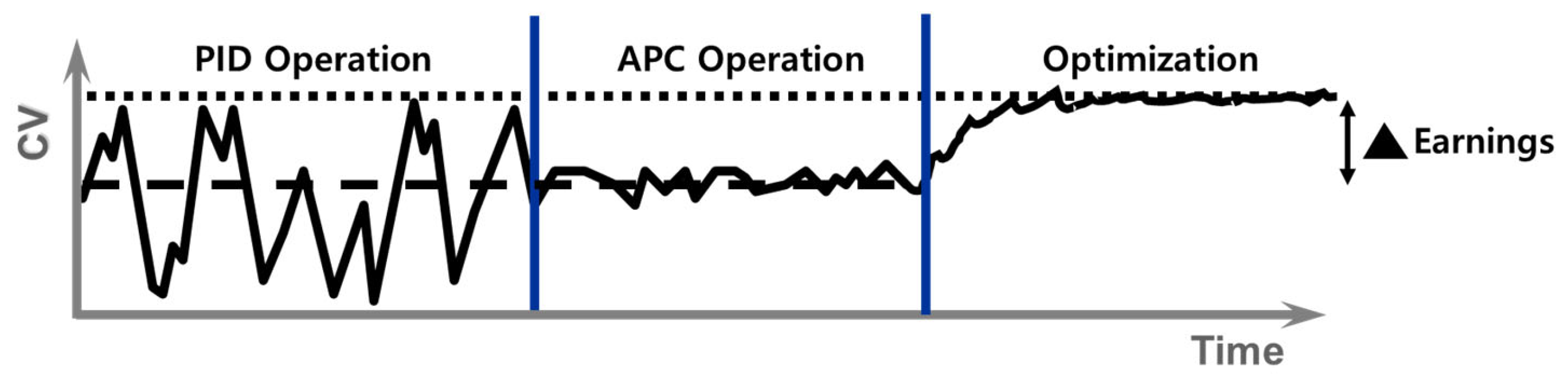
Commissioning and Performance Analytics

The reason for applying an APC system to a process is to stabilize the process and generate profits by increasing production efficiency. Therefore, it is necessary to quantitatively measure the actual profits by comparing before and after the APC system is applied. Commissioning is the stage where the actual APC is built online and operated optimally. When the APC model parameter tuning is completed, the actual profit is estimated by comparing the performance analysis of optimized operations before and after the application of the APC, as shown in Figure 6.

Figure 6. APC model commissioning and performance analytics.

2.2. Change-Point Detection

CPD is a statistical technique that searches for points of trend change in time-series data, as shown in Figure 7.

Figure 7. Example of a CPD application.

Thus, it locates the points in time-series data where the time-series characteristics, such as the mean, standard deviation, and slope, change rapidly. Figure 7 presents an example of CPD in which the vertical blue dashed lines represent the points where trend changes are detected [23,24,25].

CPD is performed by dividing the time-series data into intervals and minimizing the sum of costs per interval. Thus, CPD can be viewed as a type of partial time-series clustering problem that involves intervals of time-series data with similar characteristics [26,27,28,29]. The starting point of each interval is called the change-point. The change-detection problem for the time-series y = (y₁, y₂,……, y_t) can be formally defined as follows:

$${\mathrm{S}}^{\mathrm{*}}=\begin{array}{c}\mathrm{a}\mathrm{r}\mathrm{g}\mathrm{m}\mathrm{i}\mathrm{n}\\ \mathrm{S}\end{array}\sum _{\mathrm{s}\in \mathrm{S}}\mathrm{C}\left(\mathrm{s}\right)$$

(5)

Here, S, C, and S* denote the set of intervals, the cost function for the intervals, and the optimal set of intervals, respectively.

(1)

Pruned Exact Linear Time

The PELT algorithm is a change detection algorithm that determines the optimal interval in linear time when the number of change-points is unknown. It consists of the following steps [21,22]:

(a)

Input: time-series y, cost function C, penalty β.

(b)

Step 1: Initialize

-

Initialize z as an empty array of size T + 1

-

Initialize with Z[0] = −β

-

Initialize with L[0] = ∅

-

Initialize with x = {0}

-

Initialize with t = 1

(c)

Step 2: Update $\widehat{t}$ Z[t], L[t], and χ as follows:

-

$\widehat{t}$ ← $\genfrac{}{}{0pt}{}{{\mathrm{a}\mathrm{r}\mathrm{g}\mathrm{m}\mathrm{i}\mathrm{n}}_{}}{\mathsf{\tau }\in \mathsf{\chi }}$(Z[τ] + C($y_{\mathsf{\tau }:t}$) + β)

-

Z[$\widehat{t}$] ← Z[t] + C($y_{\widehat{t}:t}$) + β

-

L[t] ← L[$\widehat{t}$] ∪ {$\widehat{t}$}

-

χ ← {τ ∈ χ : Z[τ] + C($y_{\mathsf{\tau }:t}$) ≤ Z[t]} ∪ {$\widehat{t}$}

(d)

Step 3: Terminate the algorithm if t = τ; otherwise, increment t by 1 and return to step 2

(2)

Kernel Change-Point Detection

Kernel change-point (KCP) detection is a method of dividing intervals based on the change in the mean of each interval [22]. In KCP, data are projected onto a high-dimensional space through a measurable function known as the kernel, and change-points are detected by comparing the homogeneity of each sequence [30,31]. It is characterized by the fact that individual points are mapped using a mapping function ϕ, i.e., the cost for a set of intervals S is defined as:

$${\sum }_{\mathrm{s}\in \mathrm{S}}{\sum }_{{\mathrm{y}}_{\mathrm{t}}\in \mathrm{S}}\parallel \mathsf{\varphi }\left({\mathrm{y}}_{\mathrm{t}}\right)–\overline{\mathrm{s}}\parallel 2$$

(6)

Here, $\overline{s}$ is the average of every value in the interval s for each element in the interval s. During the mapping process, we can use the following kernel functions:

$$\parallel \mathsf{\varphi }\left({\mathrm{y}}_{\mathrm{t}}\right){\parallel }^2=\mathrm{K}({\mathrm{y}}_{\mathrm{t}}, {\mathrm{y}}_{\mathrm{t}})$$

(7)

$$\mathsf{\varphi }({\mathrm{y}}_{\mathrm{t}}) · \mathsf{\varphi }({\mathrm{y}}_{\mathsf{\tau }})=\mathrm{K}({\mathrm{y}}_{\mathrm{t}}, {\mathrm{y}}_{\mathsf{\tau }})$$

(8)

where K represents a kernel function. The most commonly used kernel functions include linear kernels and RBF kernels.

3. Overview of the Research Method

3.1. Overall Architecture

In this section, we first describe the overall structure of the analysis for estimating the APC model parameters and present the expected results of the study in terms of the estimated APC model parameters. As described in the introduction, it is important to collect data on dynamic intervals to estimate APC model parameters. Therefore, we describe the research methodology of CPD used to obtain data on dynamic intervals as well as the definition and purpose of the evaluation metric, the MAE. We also explain the rationale behind the scope of the hyper parameter grid used to determine the MAE. Overall, our analysis, consisting of the four steps shown in Figure 8, can be briefly described as follows:

Figure 8. Overall methodology of the study.

(1)

Raw data acquisition

(2)

CPD

(3)

APC model parameter estimation

(4)

Comparison of results

In this study, we used time-series data from actual petrochemical plants in Korea, which were collected through OLE for process control data access connected to distributed control systems. The names of each plant were anonymized as Plant A and Plant B, considering data security issues, and the PVs, MVs, and DVs were separated. To estimate the APC model parameters without a plant test, only the dynamic part of the data was clustered. The CPD algorithm was used to determine the dynamic intervals of the data. Among the CPD algorithms, the PELT, linear kernel, and RBF kernel techniques were used to find the hyper parameter of the dynamic region with the minimum MAE. First, the CPD algorithm was used to find the hyper parameter of the dynamic intervals with the minimum MAE, and then its value was fixed to estimate the APC model parameters, K and T, through the Levenberg–Marquardt algorithm. Finally, the estimated APC model parameters were applied to the APC control program to verify the accuracy by comparing the fitting rates of the predicted and actual values. As the MAE value of the MV and the DV for each PV becomes smaller through CPD, the fitting rate of the estimated APC model parameter shows high accuracy. The fitting rate was expected to increase as the number of MVs and DVs required for predicting and controlling the PV increased.

3.2. Designing a CPD Model

To estimate the APC model parameters from time-series data, the dynamic nature of the process must be considered. Therefore, the dynamic regions of the data must first be accurately identified. In this study, CPD algorithms such as PELT, linear kernels, and RBF kernels were used to identify fluctuating data, as shown in Figure 9. However, even with CPD techniques, accurate identification was difficult when the trend began to change. To accurately detect the beginning of a change in the trend, we must detect subtle trend changes, which is problematic because we consider most of the points to be change-points. Therefore, for any point with a trend change found using CPD, we can define the fluctuating interval as r − a to r + a where a is calculated using the following algorithm:

Figure 9. CPD techniques.

(1)

Calculate the slope θ₁ of a simple linear regression model using data from r − 1 to r + 1.

(2)

Initialize the variable a, which represents the length of the interval, to two.

(3)

Let the independent variable be t and the dependent variables be r − a to r + a. Compute the slope θ_a of a simple linear regression model with data from r − a to r + a.

(4)

If θ_a−1 × θ_a < 0 or the rate of change of the intercept of θ_a−1 relative to the intercept of θ_a is $\frac{{\left|\mathsf{\theta }\right|}_{\mathrm{a}}-{\left|\mathsf{\theta }\right|}_{\mathrm{a}-1}}{{\left|\mathsf{\theta }\right|}_{\mathrm{a}-1}}>\mathsf{\epsilon }$, return a − 1. Otherwise, increase a by one and revert to (3).

3.3. Definition and Purpose of Performance Indicators

This section describes the MAE and its suitability as a metric in CPD. The MAE is a popular metric used to determine whether a regression model has been trained properly. It can be derived by converting the difference between the actual and predicted values into an absolute value and then averaging it. A smaller value indicates better performance from the model. The formula for the MAE is as follows:

$$MAE= \frac{1}{N}\sum _{i=1}^N\left|y_{\mathit{i}}-{\mathrm{ŷ}}_{\mathit{i}}\right|$$

(9)

where $y_i$ and ${\widehat{y}}_i$ denote the actual predicted values, respectively. Because the MAE takes an absolute value, it is difficult to determine whether the regression model predicts values that are higher or lower than the actual values. However, it is easy to interpret the results because they have the same unit as the actual answer value and the predicted value. Additionally, since it takes absolute values, the results can be interpreted intuitively. In this paper, we need an intuitive indicator not to evaluate the correlation of the model but to detect the change-point of the data and indicate the difference between the predicted value and the actual value. Therefore, we use the MAE as a performance indicator for detecting change-points.

3.4. Defining and Designing Hyper Parameters

Hyper parameters are variables that are manually set in the model by a user to obtain the optimal training model. In this study, we compared the MAE of the PELT, linear kernel-based technique, and RBF kernel-based technique to identify the dynamic interval with the smallest MAE value and obtain the hyper parameters. The delay (D) and minimum segment size (MS) were used as hyper parameters to effectively detect changes in time-series data. In the absence of a rule or method for perfectly designing the hyper parameter grid mathematically, the range was set and tuned empirically. In general, the suggested ranges of the values of the hyper parameters and MS were to set the range from 0 to 10 for the hyper parameters and 5 to 20 for MS because these values rarely exceeded 10 when affected by variables in the same process. If the hyper parameter grids of D and MS have a narrow spacing, hyper parameters with good performance can be obtained; however, the computation time will increase considerably.

4. Experimental Results

4.1. Experimental Environments

To ensure the reproducibility of the experiment, we specify the experimental environment of the study:

• Hardware platform architecture: GPU-enabled laptop
• Laptop configuration: CPU Core i5-8250, quad-core processor, 8 GB RAM.
• Operating system: Windows 10.

For a fast and optimally collaborative development environment, we used the cloud-based Google Collaboratory, which provides a free Jupyter Notebook environment and is available on the cloud without installation. Google Collaboratory enables high-performance development, sharing, and computing resources. In particular, large amounts of data can be processed by this utility.

4.2. Design of the Experimental Datasets

The primary objective of the experiment was to determine data in the dynamic intervals to estimate correct APC model parameters, and the final objective was to train the model with data from only the dynamic intervals and estimate the APC model parameter with good performance. In this study, we used the time-series data obtained from two different factories, Plants A and B, at two different times, which are referred to as A-1, A-2, B-1, and B-2, respectively. The sampling time for each data point was 1 min, and the experimental data were collected over 5 days. The range of each data point was as follows:

• A-1: 23 April 2023 00:00:00 to 27 April 2023 23:59:00
• B-1: 26 March 2023 00:00:00 to 30 March 2023 23:59:00
• A-2: 30 April 2023 00:00:00 to 04 May 2023 23:59:00
• B-2: 19 April 2023 00:00:00 to 23 April 2023 23:59:00

Let A-1 and B-1 be the training data, and A-2 and B-2 be the respective test data. In addition, all four datasets described above consisted of one process variable (the PV) and two manipulative variables (the MV and the DV). The experimental trend change detection technique and its hyper parameter grid are shown in Table 1.

Table 1. CPD techniques and hyper parameter grids.

CPD Technique	Hyper Parameter Grid
PELT	MS: {5, 10, 15, 20}
	D: {0, 3, 5, 10}
Kernel-based detection [‘Linear’, ‘RBF’]	MS: {5, 10, 15, 20}
	D: {0, 3, 5, 10}

Otherwise, the hyper parameter grid evaluates the following sections:

• ε: 0.001, 0.01, 0.05, 0.1

The specific process for using the dataset is described below.

[Step 1]

To objectively evaluate the proposed Plant A and Plant B data, we divided the dataset into training and test datasets. Specifically, data recorded on the first 5 days (50%) for Plants A and B were used as training data, and the last 5 days of data (50%) were used for testing.

[Step 2]

The hyper parameters were divided into the D and the MS, and dynamic intervals were detected and identified using the PELT, the linear kernel-based technique, and the RBF kernel-based technique. We used these three methods because they are the most commonly used methods for anomaly detection in time-series data in previous studies on CPDs [32,33,34,35].

[Step 3]

The data trained by the PELT, linear kernel, and RBF kernel-based methods were used to determine the accuracy of the dynamic intervals using the MAE metric. Here, the hyper parameter of the algorithm with the smallest MAE was fixed, and the APC model parameters were estimated.

[Step 4]

The APC model parameters trained with the proposed metrics were learned by applying the following equation to the Levenberg-Marquardt algorithm [36,37]:

$$\mathrm{y}\left(\mathrm{t}\right)=\mathrm{K}\left(1-{\mathrm{e}}^{-\frac{\mathrm{t}}{\mathsf{\tau }}}\right)·\mathrm{x}\left(\mathrm{t}-\mathrm{D}\right)$$

(10)

The variables in this expression are defined as follows:

• t: Elapsed time
• y(t): PV for time t
• x(t): MV for time t (may be replaced by the DV)
• K: Gain
• τ: Time constant
• D: Delay

[Step 5]

The accuracy of the control performance was verified by comparing the fitting rates of predicted and actual values with the APC model parameter estimates obtained in Steps 3 and 4.

4.3. Results

(1) Experiment 1 (results for Plant A): For the manipulative variable MV, 10 models and hyper parameters with the smallest MAE are shown in Table 2.

Table 2. Plant A: Parameter tuning results for the MV.

Rank	Algorithms	D	MS	ε	MAE
1	Linear Kernel	10	10	0.05	8.642452
2	Linear Kernel	10	15	0.05	8.651746
3	Linear Kernel	10	5	0.05	8.656836
4	Linear Kernel	10	20	0.05	8.674863
5	Linear Kernel	5	10	0.05	8.682052
6	Linear Kernel	5	5	0.05	8.691545
7	Linear Kernel	3	10	0.05	8.693691
8	Linear Kernel	5	15	0.05	8.699134
9	Linear Kernel	3	5	0.05	8.700352
10	Linear Kernel	3	15	0.05	8.703656

For the DV, 10 models and hyper parameters with the smallest MAE are shown in Table 3.

Table 3. Plant A: Parameter tuning results for the DV.

Rank	Algorithms	D	MS	ε	MAE
1	Linear Kernel	10	20	0.01	10.73935
2	Linear Kernel	5	20	0.01	10.739671
3	Linear Kernel	3	20	0.01	10.739682
4	Linear Kernel	0	20	0.01	10.740037
5	Linear Kernel	0	15	0.01	10.741053
6	Linear Kernel	0	5	0.01	10.741164
7	Linear Kernel	0	10	0.01	10.741403
8	Linear Kernel	0	5	0.01	10.741504
9	Linear Kernel	10	5	0.01	10.742831
10	Linear Kernel	5	5	0.01	10.743456

Table 2 and Table 3 indicate that kernel-based detection with a linear kernel performs satisfactorily. The average MAEs for D, MS, and ε are listed in Table 4, Table 5 and Table 6, respectively. The distribution of performance across parameters varies significantly depending on the manipulative variables. For MVs, larger values indicate better performance, whereas for DVs, smaller values indicate better performance. This underscores the importance of tuning the appropriate parameters according to the data.

Table 4. Plant A: Average MAE for D.

Manipulative Variables	D	MAE
MV	0	9.934820
	3	9.914994
	5	9.905677
	10	9.820333
DV	0	11.741451
	3	12.000861
	5	11.999641
	10	11.997169

Table 5. Plant A: Average MAE for MS.

Manipulative Variables	MS	MAE
MV	5	9.876135
	10	9.904980
	15	9.927402
	20	9.867307
DV	5	11.864946
	10	12.038425
	15	11.882389
	20	11.953361

Table 6. Plant A: Average MAE for ε.

Manipulative Variables	ε	MAE
MV	0.01	9.898091
	0.05	9.579578
	0.10	10.204200
DV	0.01	11.386267
	0.05	12.186671
	0.10	12.231404

As shown in Table 7, the linear kernel-based change detection algorithm performs well for both the MV and DV. Based on the best-performing linear kernel-based hyper parameters of D = 10, MS = 10, and ε = 0.05 for the MV, the Levenberg-Marquardt algorithm estimated the model parameters of the MV for the PV as K = 15.3188 and τ = 0.3221. Furthermore, based on the best-performing linear kernel-based hyper parameters for D = 5, MS = 10, and ε = 0.01, the estimated model parameters of the DV for the PV were K = 22.85 and τ = 0.0309. The graphical representation of the APC model parameters estimated based on the best-performing model for the operational variables, MV and DV, and the result of measuring the fitting rate using the APC model program are shown in Figure 10, Figure 11 and Figure 12. Three intervals of approximately 200 min in length were randomly selected from the evaluation data intervals of Plant A. In Figure 10, Figure 11 and Figure 12, the x-axis represents time, and the y-axis represents the range of the PV.

Table 7. Plant A: Average MAE for various algorithms.

Manipulative Variables	Algorithms	MAE
MV	Linear Kernel	9.399081
	RBF Kernel	9.507844
	PELT	10.774943
DV	Linear Kernel	11.443224
	RBF Kernel	12.540117
	PELT	11.821000

Figure 10. (Section 1) Fitting rate of the PV with the estimated APC model parameters at Plant A.

Figure 11. (Section 2) Fitting rate of the PV with the estimated APC model parameters at Plant A.

Figure 12. (Section 3) Fitting rate of the PV with the estimated APC model parameters at Plant A.

We measured the fitting rate of the estimated APC model parameter to the predicted and actual values using the APC model program and obtained the following results:

• (Section 1) PV fitting rate with the estimated APC model parameters (MV+DV): 81.9%
• (Section 2) PV fitting rate with the estimated APC model parameters (MV+DV): 81.04%
• (Section 3) PV fitting rate with the estimated APC model parameters (MV+DV): 95.35%

(2) Experiment 2 (results for Plant B): For the MV, 10 models and hyper parameters with the smallest MAE are shown in Table 8.

Table 8. Plant B: Parameter tuning results for the MV.

Rank	Algorithms	D	MS	ε	MAE
1	RBF Kernel	0	10	0.01	45.629945
2	RBF Kernel	0	5	0.01	45.647986
3	RBF Kernel	0	20	0.01	45.813426
4	Linear Kernel	0	5	0.10	46.103089
5	Linear Kernel	0	5	0.05	46.117504
6	RBF Kernel	0	15	0.01	46.118124
7	RBF Kernel	0	5	0.10	46.121928
8	RBF Kernel	10	10	0.01	46.134523
9	RBF Kernel	5	10	0.01	46.136264
10	RBF Kernel	0	15	0.10	46.147291

For the DV, 10 models and hyper parameters with the smallest MAE are shown in Table 9.

Table 9. Plant B: Parameter tuning results for the DV.

Rank	Algorithms	D	MS	ε	MAE
1	RBF Kernel	3	20	0.01	4.110627
2	RBF Kernel	5	20	0.01	4.192519
3	RBF Kernel	0	20	0.01	4.196660
4	RBF Kernel	10	20	0.01	4.200493
5	PELT	0	20	0.10	4.216778
6	Linear Kernel	0	10	0.01	4.231443
7	Linear Kernel	3	10	0.01	4.234592
8	PELT	3	20	0.10	4.269921
9	Linear Kernel	5	10	0.01	4.270220
10	PELT	5	20	0.10	4.274902

The averages of the MAE for D, MS, and ε are presented in Table 10, Table 11 and Table 12, respectively. The parameterized performance distributions differ significantly depending on the manipulative variables.

Table 10. Plant B: Average MAE for D.

Manipulative Variables	D	MAE
MV	0	47.014508
	3	47.014508
	5	47.703097
	10	47.672040
DV	0	4.402237
	3	4.417269
	5	4.420273
	10	4.431750

Table 11. Plant B: Average MAE for MS.

Manipulative Variables	MS	MAE
MV	5	47.090598
	10	47.331090
	15	47.803609
	20	47.881317
DV	5	4.425821
	10	4.406654
	15	4.439160
	20	4.404137

Table 12. Plant B: Average MAE for ε.

Manipulative Variables	ε	MAE
MV	0.01	47.603724
	0.05	47.531555
	0.10	47.444681
DV	0.01	4.402237
	0.05	4.339782
	0.10	4.482717

A comparison of the average MAE for various algorithms is presented in Table 13.

Table 13. Plant B: Average MAE for various algorithms.

Manipulative Variables	Algorithms	MAE
MV	Linear Kernel	47.092989
	RBF Kernel	46.742333
	PELT	48.744638
DV	Linear Kernel	4.399071
	RBF Kernel	4.498206
	PELT	4.356370

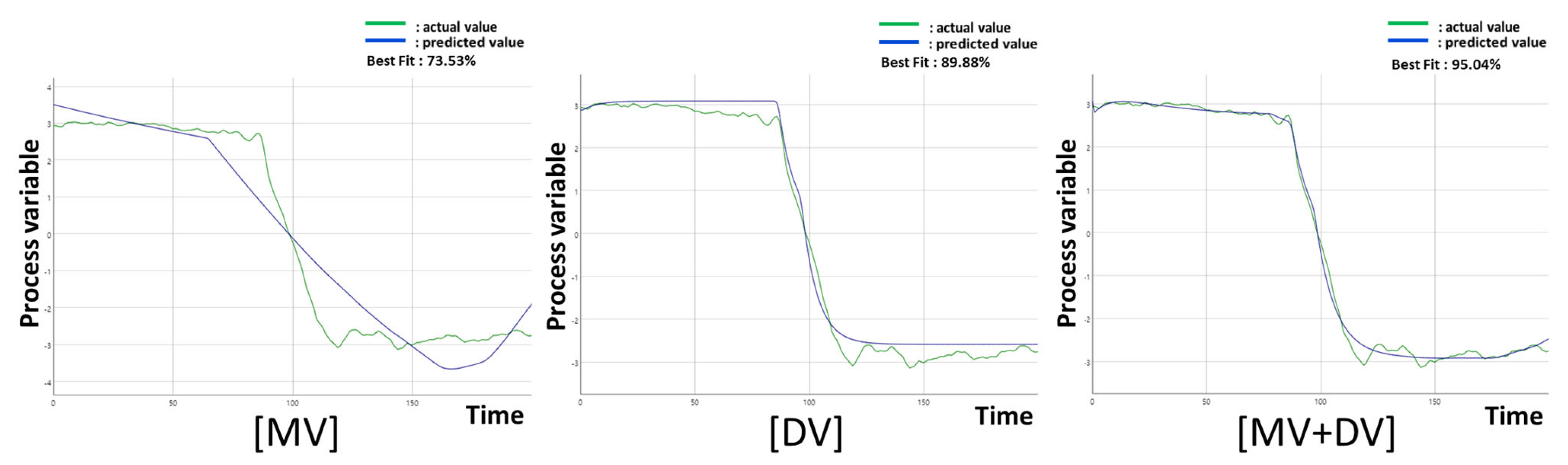
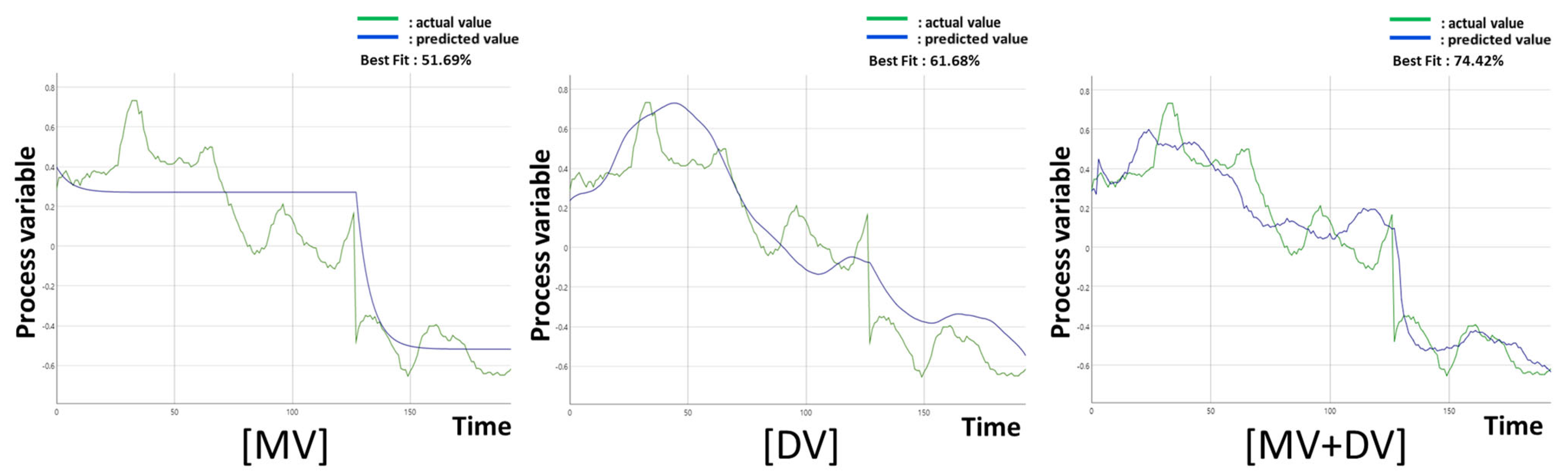
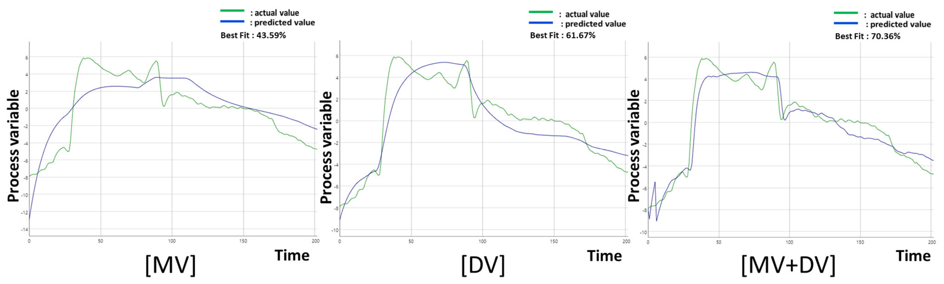
As shown in Table 13, the most appropriate algorithm depends on the manipulative variables. In addition, the difference in performance across the manipulative variables is nearly an order of magnitude. This suggests that the performance difference can be large, depending on the variable used to predict the control variable. Based on D = 0, MS = 5, and ε = 0.05, that is, the linear kernel-based hyper parameters that performed the best for the MV, the model parameter estimation of the MV for the PV using the Levenberg-Marquardt algorithm yielded K = 2.644706 and τ = 0.038512. Based on D = 0, MS = 15, and ε = 0.1, the best-performing hyper parameter based on the PELT technique for the DV, the model parameter estimates of the DV for the PV yielded K = 0.9556 and τ = 0.0337. A graphical representation of the APC model parameters estimated based on the best-performing model for the MV and DV and the fitting rate measured by the APC program are shown in Figure 13, Figure 14 and Figure 15. Three intervals of approximately 200 min in length were randomly selected from the evaluation data intervals of Plant B. In Figure 13, Figure 14 and Figure 15, the x-axis represents time, and the y-axis represents the range of the PV.

Figure 13. (Section 1) Fitting rate of the PV with the estimated APC model parameters at Plant B.

Figure 14. (Section 2) Fitting rate of the PV with the estimated APC model parameters at Plant B.

Figure 15. (Section 3) Fitting rate of the PV with the estimated APC model parameters at Plant B.

We measured the fitting rate of the estimated APC model parameters to the predicted and actual values using the APC program and obtained the following results:

• (Section 1) PV fitting rate with the estimated APC model parameters (MV+DV): 95.04%
• (Section 2) PV fitting rate with the estimated APC model parameters (MV+DV): 74.42%
• (Section 3) PV fitting rate with the estimated APC model parameters (MV+DV): 70.36%

5. Conclusions

APC model parameters play a crucial role in APC control. Many papers have utilized CPD in various fields, and the results have been excellent. However, no study has been conducted to estimate APC model parameters from dynamic intervals of data identified by CPD. In this study, we identify dynamic intervals of data by CPD from the time-series data of the petrochemical process industry. Then, the fitting rate validation of the APC model parameters estimated from the dynamic intervals allowed us to verify the accuracy of the model with significance. In this study, PELT, linear kernel-based, and RBF kernel-based techniques were applied to CPD to evaluate the MAE of the dynamic intervals, as described in Section 3. The results show that the linear kernel-based method yields the best results for the MV and DV of Plant A, the RBF kernel-based method is the best for the MV of Plant B, and the PELT method is the best for the DV of Plant B. Because the variables can be current set or valve values of flow, pressure, temperature, and so on in petrochemical processes, the performance of the models may differ considerably depending on the variables used to predict the control variables. The experimental results in Section 4 show that the PV control method that considers both the MV and DV rather than controlling the PV with the MV or DV alone has the highest fitting rate. Thus, by selecting the hyper parameters in the dynamic intervals with the minimum MAE, the estimated APC model parameters were determined for the fitting rate with the predicted and actual values using the APC program. The average fitting rates were 86.09% and 79.94% for Plants A and B, respectively. The final fitting rate validation confirmed the high accuracy of the dynamic interval identification and APC model parameter estimation performance with CPD. This shows that it is possible to estimate APC model parameters from dynamic intervals determined using CPD without a plant test, which can be negatively affected by engineer skill.

In the future, extended experiments with more process data are needed to increase the reliability of the results. Further research is needed to determine whether the three CPD techniques performed in this study are the most optimized methods. Therefore, a study should be conducted to compare the MAE of dynamic intervals utilizing the CPD method in addition to the PELT, linear kernel, and RBF kernel methods to increase the reliability of the results of this study. In addition, since the APC model parameters estimated in this study are theoretical values, further research should be conducted to verify whether the APC system operates normally by applying it to a real process and whether the calculated model can reduce process deviation compared to the PID system.