A Method for Judging the Effectiveness of Complex Tight Gas Reservoirs Based on Geophysical Logging Data and Using the L Block of the Ordos Basin as a Case Study

Abstract

As an important unconventional oil and gas resource, the tight gas reservoir faces many technical challenges due to its low porosity, low permeability, and strong heterogeneity. Among them, the accurate definition of effective reservoirs and ineffective reservoirs in tight gas reservoirs directly affects the formulation and adjustment of subsequent development plans. This paper proposes a reservoir effectiveness identification method based on double factors based on conventional geophysical logging data and core experimental data. The double factors considered are based on the logging response and physical parameters of the reservoir. The identification factor $F_1$ is obtained by using the difference in the logging response values of the natural gamma logging curve, compensated density logging curve, and acoustic time difference logging curve in different reservoirs combined with mathematical operation, and the identification factor $F_2$ is calculated by using porosity parameters combined with Archie’s formula. The validity of the reservoir can be judged by the intersection of the above double factors. This method is applied to the Shihezi Formation in the L block, and the applicability of the double factors is compared and analyzed using the traditional method. The results show that the method has strong applicability in tight gas reservoirs and that the accuracy rate reaches 96%. Compared with the direct use of the porosity lower limit method, the accuracy of the judgment is significantly improved, and the calculation is simple, easy to implement, and unaffected by mud invasion. For study areas with different geological backgrounds, the process of this method can also be used to determine the effectiveness of the reservoir. The reservoir effectiveness identification method proposed in this paper has practical engineering significance and lays a solid foundation for subsequent fluid property identification, production calculation, and development plan formulation and adjustment.

1. Introduction

Currently, with the continuous development of oil and gas fields, conventional oil and gas resources reserves are gradually reducing, and the existence of technical bottlenecks in the development of residual oil, where further breakthroughs are still needed, have increased the difficulty of oil exploration and development, establishing exploration objects, and the development of more complex resource storage conditions. Complex oil and gas reservoirs, such as low- and extra-low-permeability reservoirs, high- and extra-high-water-bearing reservoirs, and low-resistivity reservoirs, have now become the primary exploration targets and are likely to continue to be in the future as well. Among them, tight gas, a kind of coal measure gas, is a significant unconventional oil and gas resource that has received a lot of attention internationally [1,2,3,4,5], and many countries have invested a lot of financial resources into the exploration and development of tight gas.

Tight gas reservoirs have the characteristics of low porosity, low permeability, and strong heterogeneity [6,7,8,9]. Compared with conventional reservoirs, the development of tight reservoirs faces greater difficulties and challenges; the research methods applied in conventional reservoirs cannot meet the production requirements in tight reservoirs, and the poor evaluation of parameters during the exploration period can have various effects on later production [9]. Among them, the identification of reservoir effectiveness as a key task in the identification of fluid property, reserve calculation, and the formulation of development plans [10,11,12,13,14] has always been a research hotspot and a major problem for scholars in related fields internationally, especially for complex reservoirs such as tight gas reservoirs.

An effective reservoir is one that can store fluid and allow it to flow, has additional supercritical porosity and permeability, and can produce liquid with an industrial value under the conditions of existing process technology. Compared with the effective reservoir, the ineffective reservoir can only store fluid, but the fluid cannot flow within it (or the fluid cannot flow under the current technological conditions), and it does not have industrial production value [13,15,16]. Therefore, the effectiveness of accurate reservoir identification lays a foundation for subsequent reservoir fluid property identification, which can improve the efficiency of development and production. Considering the abundance of logging data in actual oil and gas fields and the characteristics of high vertical resolution, high performance–price ratio, and reliability of logging data, which can lay the data foundation for parameter calculation, the validity identification of reservoirs in oil and gas reservoirs is mostly carried out by determining the lower limit of physical parameters, such as the effective porosity of effective reservoirs, and then combining this with logging data for parameter calculation. Previously, most scholars used porosity–permeability crossplots to determine the lower limit of the physical properties of the effective reservoirs [13,17,18,19], which is simple, convenient, clear, and intuitive, but due to the coupling of physical parameters, especially permeability, the evaluation accuracy of this parameter is limited, and the practical use effect in the application process is not satisfactory. Wang et al. improved this type of physical property method by classifying the pore throat structure through piezometric data, establishing the relationship between permeability and porosity separately, and then evaluating the lower limit of the physical properties of effective reservoirs [16], and this method improved the accuracy of the porosity–permeability crossplot method. Harfoushian and Suriyanto suggested the use of advanced formation test apparatuses to measure in situ permeability [20], which led to a significant improvement in the accuracy of the lower limit of effective reservoir properties and achieved good results when applied to the Acme West gas field in the Carnarvon basin. However, the time cost and economic cost of using such formation test apparatuses are extremely high; therefore, considering the economics, this is difficult to promote on a large scale in the whole work area. Subsequently, with the development of mathematical geological methods and machine learning methods, such as fuzzy classifier fusion, Bayesian theory, and artificial neural networks, etc., these methods have also been gradually applied to determine the lower limits of the effective reservoir properties [21,22,23]. As a powerful classification tool, it is not only suitable for high-dimensional data but also simple, easy to understand, and capable of processing a large amount of data in a short time. However, the accuracy and stability of these methods are difficult to guarantee, as is the effectiveness of such methods, due to the difficulty of providing physical meaning and the inability to be transparent in the model construction process. Mehdipour et al. used the water saturation parameters determined by geophysical logging data to determine the lower physical limit of the effective reservoir, plotted the frequency distribution of water saturation, found the lower limit of water saturation (the value with the highest water saturation and the lowest frequency) via its morphological characteristics, divided the porosity into two categories using this lower limit, plotted the frequency distribution separately, and used the intersection of the two curves as the lower limit of porosity [24]. This method has achieved good results in the Ilam Formation of an oil field in Iran, but it is difficult to determine the lower limit of water saturation. In addition, NMR technology can directly evaluate the porosity, permeability, pore structure, and other reservoir information related to reservoir physical properties, so it is feasible to use this technology to determine the lower limit of effective reservoir physical properties [25,26,27]. However, this method is based on core experiments and cannot be applied without relevant experimental data. It is difficult to use directly in development wells with limited core quantity and no supporting NMR logging data. On the basis of fully considering economic factors such as the balance of payments, drilling costs, surface infrastructure costs, oil prices, etc., Yang T et al. developed a complete set of methods and processes for determining the lower limit of the effective reservoir’s physical properties by using core description, core analysis, thin sections, and other data. However, in order to obtain an accurate lower limit of the physical properties, it is necessary to attain accurate oil saturation and sufficient well test data [11]. Mehdi Qassamipour et al. divided effective reservoirs by establishing oil and gas rate profiles to determine oil and gas production limits [10]. However, this method is not suitable for natural gas reservoirs because it is based on Darcy’s flow equation. Yang Z et al. used the experimental method to establish a new method for calculating the thickness of the bound water film and determined the lower limit of the pore throat radius by the thickness of the bound water film to obtain the lower limit of the physical properties of the effective reservoir [28]. The premise of using this method is to have enough core experimental samples. In addition, Qin et al. evaluated the effectiveness of reservoirs by analyzing rock facies [29], but this method requires a large amount of geological data and rich geological experience in advance to achieve good results.

In summary, most of the previous solutions to the problem of reservoir effectiveness division involved determining the lower limit of reservoir physical properties by evaluating the physical parameters of the reservoir (porosity, permeability, and water saturation) or the minimum pore radius and then evaluating the effectiveness of the reservoir based on the corresponding parameters. Most of the above methods used a single parameter for evaluation. Even if the porosity and permeability are evaluated simultaneously, the permeability is mostly fitted by porosity; there is little difference in nature. Therefore, this paper uses Block L of the Ordos Basin as a case study and, combined with conventional geophysical logging data, proposes a method for reservoir validity identification based on the double-factor method. Logging curves sensitive to effective reservoir response, namely natural gamma curve, compensated density curve, and acoustic time difference curve, are used for mathematical calculation to construct identification factor $F_1$. Porosity and Archie’s formula are used to construct identification factor $F_2$, and a more effective evaluation process is established by intersecting the double factors and providing the judgment range to identify effective reservoirs. This process has been applied to dozens of wells in L block and achieved good application results, and the method in this paper only requires geophysical logging data plus rock electric parameters in the same block for completion and has low requirements with respect to experimental data types. While ensuring the effectiveness of the method, it also takes into account the actual cost and lays the foundation for further fluid identification work and production calculation.

2. Geological Overview

The Ordos Basin is located at the junction of the stable area in eastern China and the active zone in western China. It is surrounded by orogenic belts and is a rectangular syncline with a north–south strike and a slow east and steep west. It is composed of six tectonic units: Yimeng uplift in the north, Weibei uplift in the south, the western margin thrust belt is in the middle from west to east, the Tianhuan depression belt, the Yishan slope belt, and the Jinxi flexural fold belt (Figure 1). The faults in the basin are mainly strike-slip faults under the action of tectonic stress [30,31].

Block L is located in the Jinxi flexure zone of the Ordos Basin, and its administrative division is located in the X and L counties of the west of the Shanxi Province. Tight gas layers are developed in multiple exploration strata in Block L, including the Upper Paleozoic Permian Shiqianfeng Formation, Upper Shihezi Formation, Lower Shihezi Formation, Taiyuan Formation, and Carboniferous Benxi Formation. The reservoir rock composition in the L area is complex, mainly developing feldspar lithic sandstone, lithic feldspar sandstone and lithic sandstone, and a small amount of lithic quartz sandstone and quartz sandstone. The rock debris composition of the L block is mainly volcanic rock and pyroclastic rock; the interstitial material is mainly composed of clay, sericite, and calcite; and the content of conductive minerals is low. The rock structure is mainly dense, the sorting is moderate and poor, and there are slight differences in different layer groups. Additionally, the support type is mainly particle support; there is a common, visible quartz secondary enlargement phenomenon; the degree of weathering alteration is deep; the roundness is mainly sub-round; and the rock reservoir space is mainly residual intergranular pore and dissolved intergranular pore, followed by fracture pore. The porosity of the Upper Paleozoic sandstone in the L area is about 0.3~21.5%, with an average of 7.3%, and the permeability is about 0.001~89.6 mD, with an average of 0.33 mD. Coal seams and dark mudstones are developed, mainly type III and type II2 kerogen. The tight sandstone reservoirs in the study area are rich in natural gas resources.

The main horizon studied in this paper is the Shihezi Formation in the L block. The geophysical logging data of each well in the block were collected. At the same time, the core experimental data of the exploration wells in the study block were collected, and the logging data of the layers with DST conclusions and production conclusions in the sample wells were extracted. In order to expand the number of samples, multiple sets of data sampling were carried out on the reservoir.

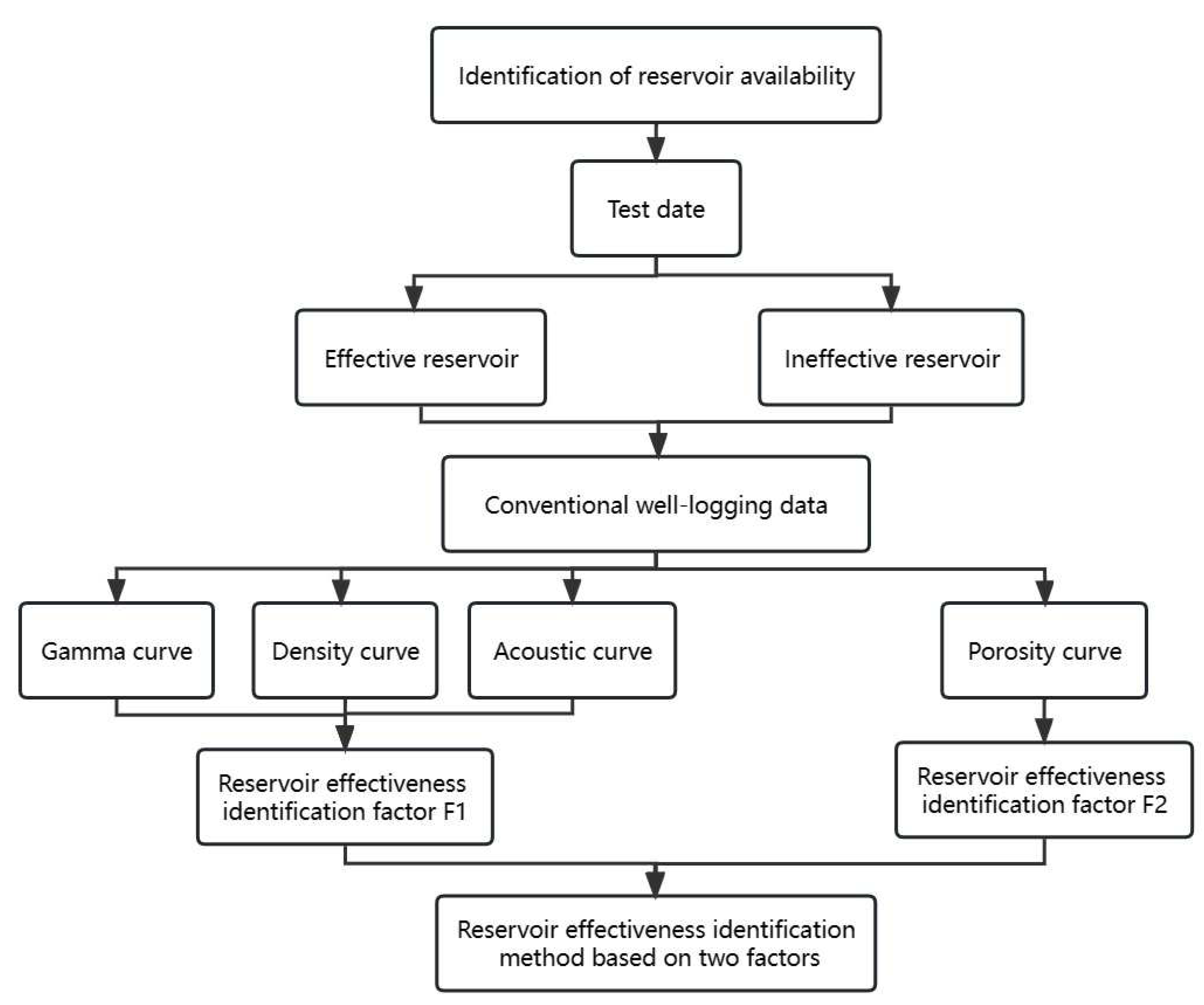
3. Principle of the Method

Considering the abundance of geophysical logging data and the subsequent application effect, in this paper, two reservoir effectiveness identification factors are constructed based on geophysical logging data and the reservoir parameters evaluated based on the geophysical logging data.

3.1. Reservoir Effectiveness Identification Factor F1

The construction principle of the reservoir effectiveness identification factor $F_1$: Based on geophysical logging data, the type of logging curve sensitive to the effective reservoir response is preferred by analyzing the logging response characteristics of the effective and ineffective reservoirs, and this sensitivity is amplified by using the mathematical method to highlight the logging response variation in the trend of the effective reservoirs to distinguish the effective and ineffective reservoirs. The specific expression of $F_1$ is shown in Equation (1):

$$F_1=\frac{A_1\times A_2\times \cdots \times A_n}{B_1\times B_2\times \cdots \times B_n}$$

(1)

where $A_n$ and $B_n$ represent the types of curves with opposite logging response trends in the effective and ineffective reservoirs, respectively. It should be noted that there is no explicit requirement for the sequence of logs in the numerator and denominator; only the logging curves in the numerator and denominator have opposite trends when facing the effective and ineffective reservoirs. In this paper, the logging curve with an increasing trend of logging response in the effective reservoir is placed in the numerator of Equation (1), and the logging curve with a decreasing trend of logging response is placed in the denominator, which can improve the differentiation between effective and ineffective reservoirs in the logging response, and then the effectiveness of the reservoir is identified.

The geophysical logging data collected for the study area data include the well diameter logging curve, compensated neutron logging curve, acoustic time difference logging curve, natural gamma logging curve, array-induced resistivity logging curve, PE logging curve, natural potential logging curve, and compensated density logging curve. In this paper, the response characteristics of the above logging curves are analyzed using boxplots in conjunction with actual gas test findings and production data, and the results are shown in Figure 2. Each graph in Figure 2 contains two box plots, which are the distribution of the logging response for effective and ineffective reservoirs and the distribution of the logging response for reservoirs with different fluid properties in effective reservoirs, i.e., the source of the logging response for effective reservoirs. As shown in Figure 2a,b,f–h, the caliper logging curves, compensated neutron logging curves, M2RX (array induction logging with a detection depth of 120 inches) curves, PE curves, and natural potential logging curves do not differ significantly in the response characteristics of the effective and ineffective reservoirs. Combined with the analysis of Figure 2c–e, it can be seen that the logging response characteristics of the compensated density logging curve, acoustic time difference logging curve, and natural gamma logging curve in the effective reservoir and ineffective reservoir are obviously different, which indicates that the compensated density logging curve, acoustic time difference logging curve, and natural gamma logging curve are very sensitive to the division of the effective reservoir [32]. In the effective reservoir section, the response pattern of the geophysical logging data is as follows: low natural gamma value, small density logging response value, and large acoustic time difference logging response value. In the ineffective reservoir section, the logging response pattern is as follows: high natural gamma value, large compensation density logging response value, and small acoustic time difference logging response value, which is mainly due to the fact that the mud content of the ineffective reservoir is usually higher than that of the effective reservoir, resulting in high natural gamma. The ineffective reservoir is often denser and contains no or very little fluid, resulting in a higher reservoir density in the ineffective reservoir than in the effective reservoir. Similarly, for the acoustic time difference logging series, the ineffective reservoir is denser and, combined with the propagation characteristics of acoustic waves, the acoustic waves in the ineffective reservoir travel faster, corresponding to a lower acoustic time difference logging response value than the acoustic time difference logging response value in the effective reservoir.

By substituting the above three logging curves of natural gamma, compensated density, and acoustic time difference into Formula (1) according to their response characteristics, the response characteristics of effective reservoirs can be amplified, that is, the reservoir effectiveness identification factor $F_1$ in this paper.

3.2. Reservoir Effectiveness Identification Factor F2

The logging response of the resistivity series corresponding to the ineffective reservoir studied in this paper has no obvious discrimination compared with the logging response of the resistivity series of the effective reservoir, and there is a “low resistance” phenomenon. In order to further combine the reservoir’s physical properties and resistivity, this paper forms a new identification factor by reconstructing the resistivity curve.

The porosity calculation model is constructed by core porosity and compensation density logging curves, and it is assumed that the reservoir in this paper satisfies Archie’s formula and is full of water, i.e., a theoretical resistivity curve with 100% water saturation is calculated to amplify the difference in porosity in different reservoirs [33,34].

The basic form of Archie’s formula is shown in Equations (2) and (3) [35]:

$$F=\frac{a}{{\varphi }^m}=\frac{R_o}{R_w}$$

(2)

$$I=\frac{b}{S_w{}^n}=\frac{R_t}{R_o}$$

(3)

where $F$—formation factor, dimensionless; $a$—cementation constant, dimensionless; $m$—cementation index, dimensionless; $\varphi$—porosity, fraction; $R_o$—resistivity of the formation saturated with brine water, Ohm.m; $R_w$—formation water resistivity, Ohm.m; $I$—resistance increase coefficient, dimensionless; $b$—saturation constant, dimensionless; $S_w$—water saturation, fraction; and $R_t$—formation resistivity, Ohm-m.

By a simple transformation of Archie’s formula, Equation (4) can be obtained:

$$R_t=\frac{ab{R}_w}{{\varphi }^m{S}_w{}^n}$$

(4)

As can be seen from Equation (4), when the other condition is constant, the physical properties of the reservoir are worse, the porosity is lower, and the resistivity of the corresponding formation is higher when it is full of water. The physical properties of the ineffective reservoir are much worse than those of the effective reservoir, i.e., the resistivity of the ineffective reservoir at full water content should be much greater than that of the effective reservoir at full water content. Therefore, this paper constructs a resistivity curve of 100% saturated formation water by calculating the porosity curve and combining Archie’s formula as the reservoir effectiveness identification factor $F_2$. Since $F_2$ amplifies the difference in the porosity of different reservoirs, the $F_2$ of the effective reservoir should be significantly lower than that $F_2$ of in the ineffective reservoir, as shown in Equation (5):

$$F_2=\frac{ab{R}_w}{{\varphi }^m}$$

(5)

To summarize, this paper proposes a new process for determining reservoir effectiveness (Figure 3). Firstly, ineffective and effective reservoirs are classified based on gas test data, and then the response characteristics of these two types of reservoirs on conventional logging curves are analyzed, from which three logging curves sensitive to the reservoir effectiveness response are selected: natural gamma curve, compensated density curve, and acoustic time difference curve. These three logging curves are used to construct the effectiveness identification factor $F_1$ via mathematical operation. Next, a theoretical resistivity curve is reconstructed as the effectiveness identification factor $F_2$ by taking into account the physical properties of the reservoir and using the porosity and Archie’s formula. Finally, a new reservoir effectiveness identification chart is constructed based on the double factors. Through the map, the range of the effective reservoirs and ineffective reservoirs is delimited, respectively, and then the effectiveness of the reservoir is identified.

4. Results and Discussion

4.1. Results

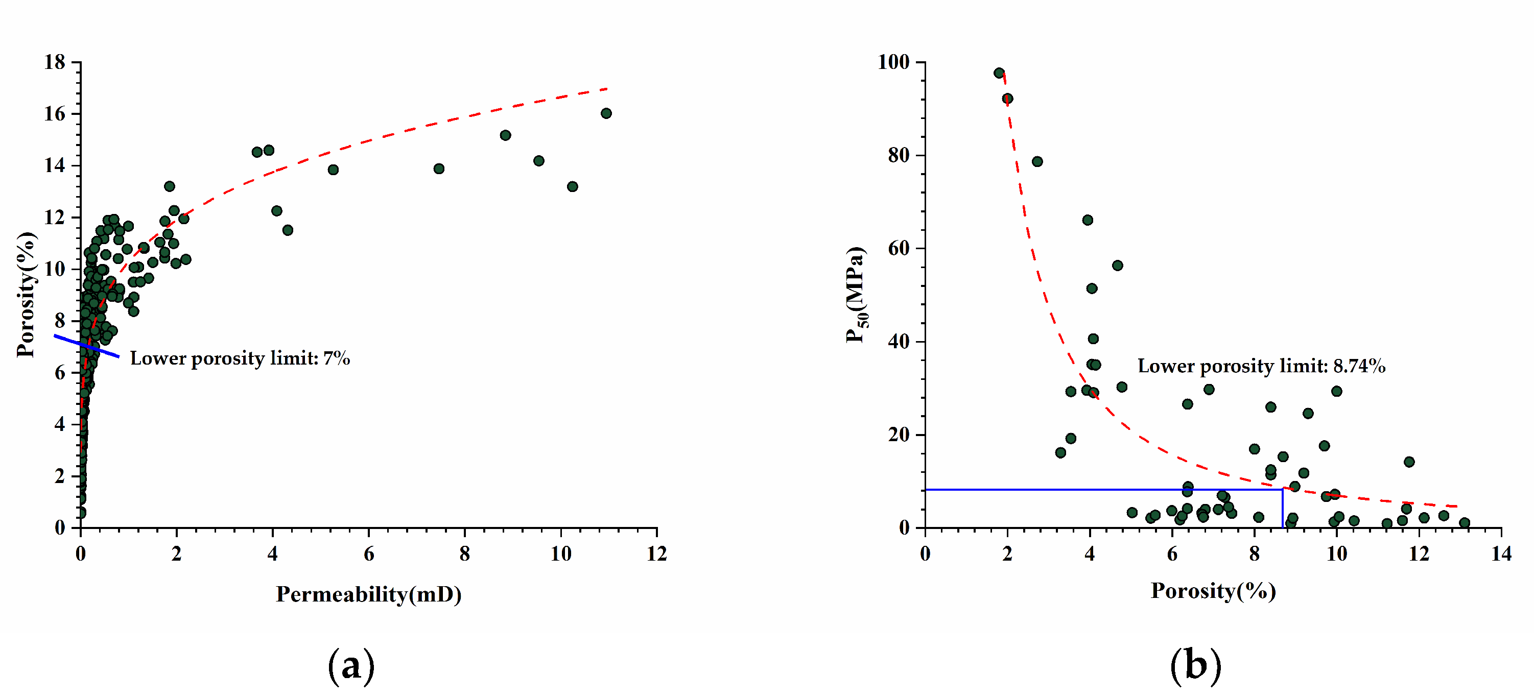
4.1.1. Model Building Process

1. The natural gamma logging curve, compensated density logging curve, and acoustic time difference logging curve are used to establish the reservoir effectiveness identification factor $F_1$. To eliminate the effect of the different curve scales on the factor amplification, the response values of these three logging curves are first normalized separately, as shown in Equation (6).

$$X^{\ast }=\frac{X-X_{\min }}{X_{\max }-X_{\min }}$$

(6)

where $X^{\ast }$ is the normalized logging response, $X$ is the original logging response, $X_{\min }$ is the smallest logging response among the collected reservoir response data, and $X_{\max }$ is the largest logging response among the collected reservoir response data. The curves processed in this paper are the natural gamma logging curve, the compensated density logging curve, and the acoustic time difference logging curve.

The normalized data are then brought into Equation (1) for the effective reservoir identification factor $F_1$. The response values of natural gamma logging and compensated density logging in the effective reservoir are lower than the response values of the corresponding curves in the ineffective reservoir, and for the acoustic time difference logging response values, the effective reservoir is higher than the ineffective reservoir. Therefore, the normalized acoustic time difference logging response value is placed in the denominator, and the normalized compensation density logging response value and natural gamma logging response value are placed in the numerator, as shown in Equation (7):

$$F_1=\frac{G{R}^{\ast }\times ZDE{N}^{\ast }}{D{T}^{\ast }}$$

(7)

Considering that the denominator is the single variable of the normalized acoustic time difference logging response, to further amplify the sensitivity of the natural gamma logging response, the compensated density logging response, and the acoustic time difference logging response to the effective reservoir, the normalized acoustic time difference value in the denominator position is squared to obtain $F_1^{\prime }$ and replaced with $F_1$, as shown in Equation (8):

$$F_1^{\prime }=\frac{G{R}^{\ast }\times ZDE{N}^{\ast }}{{\left(D{T}^{\ast }\right)}^2}$$

(8)

2. Using the porosity parameter combined with Archie’s formula to construct the reservoir effectiveness identification factor $F_2$, firstly, the porosity calculation formula is obtained by fitting the core porosity with the compensated density logging curve (Figure 4), as shown in Equation (9).

$$\varphi =-55.4\times DEN+150.19$$

(9)

The results calculated by Equation (9) are substituted into Equation (5); at this time, the value of formation water resistivity $R_w$ in Equation (5) is determined by the formation water analysis data of the study block, taken as $R_w=0.083\Omega \cdot \mathrm{m}$. The values of a, b, and m are determined according to the petrographic experimental data and fitted to the formation factor $F$ and porosity $\varphi$ (Figure 5a) to obtain a = 3.8136 and m = 1.383 and fitted to the resistivity increase factor $I$ and water saturation $S_w$ (Figure 5b) to obtain b = 1.0403 and n = 1.525. It should be noted that, at this point, the parameters obtained by petrographic experiments, especially the cementation index m, combined with the porosity, play an amplifying role and can be used if there is a slight non-Archie phenomenon in the petrographic data. The reservoir effectiveness identification factor $F_2$ can be found by substituting the obtained petrophysical parameters into Equation (5).

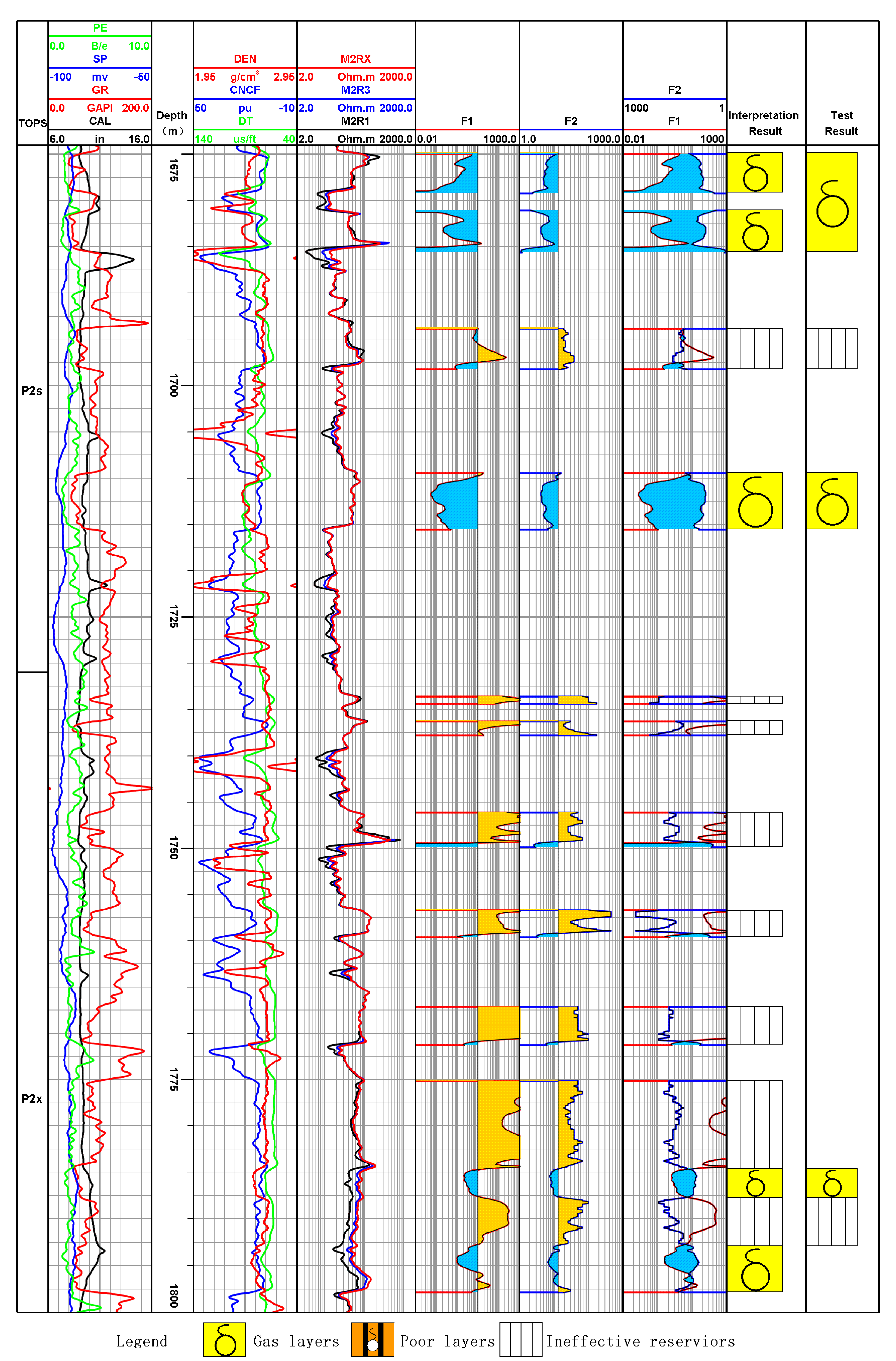
4.1.2. Application Effect

The double-factor-based reservoir effectiveness identification method was applied to 26 test layers in 16 wells in block L. Then, the reservoir effectiveness identification factor $F_1^{\prime }$ was used as the X-axis, and the reservoir effectiveness identification factor $F_2$ was used as the Y-axis to make the crossplot; and the scale was chosen as the logarithmic scale, and the results are shown in Figure 6.

Figure 6 shows that the calculated value of $F_1$ for the ineffective reservoir is significantly higher than that of $F_1$ for the effective reservoir. The value of the reservoir effectiveness identification factor $F_2$ is also higher than that of the effective reservoir, i.e., the data points of the ineffective reservoir are located at the upper right of the crossplot, and those of the effective reservoir are located at the lower left of the crossplot. The compensated density logging response and natural gamma logging response of the ineffective reservoir are higher, and the acoustic time difference logging value is smaller than that of the effective reservoir. The reservoir effectiveness identification factor $F_1$ is a fractional equation, the denominator of which is the value of the logging curve with an upward trend in the effective reservoir, and the numerator is the logging curve with a downward trend in the effective reservoir, plus the square of the numerator, so the value of the reservoir effectiveness identification factor $F_1$ of the ineffective reservoir is obviously greater than that of the effective reservoir. The physical properties of the ineffective reservoir are worse than that of the effective reservoir, so the resistivity response value of 100% saturated formation water calculated in the ineffective reservoir is larger, i.e., the results of practical application are consistent with the theory. By analyzing the location of the effective and ineffective reservoir samples in the plate, the range was divided by combining the perception of actual production, as shown in

Table 1. Range of values of $F_1$ and $F_2$ in the effective reservoir.

Reservoir Effectiveness Identification Factor	Effective Reservoir
$F_1$	0 < $F_1$ < 10
$F_2$	0 < $F_2$ < 13

. The effectiveness of the reservoir can be effectively determined by the chart, and the application effect in the new well is shown in Figure 7; the confusion matrix when the method is applied in the new well is given, as shown in

Table 2. Confusion matrix of the double-factor method in reservoir applications.

Accuracy (96%)
Test Results	Effective Reservoir	Ineffective Reservoir
Effective reservoir	21 (100%)	0 (0%)
Ineffective reservoir	1 (20%)	4 (80%)

, and a graph of the effect of a new well is shown (Figure 8). Ten tracks are shown in Figure 8. The first track is a stratigraphic track containing formation information; the second track is a lithology logging track containing the curves of the lithology logging series, including the natural gamma logging curve, natural potential logging curve, photoelectric absorption cross-section index curve, and well diameter curve. The third track is a depth track; the fourth track is a porosity logging track, which contains the curves of the porosity logging series, with compensated density logging curves, compensated neutron logging curves, and acoustic time difference logging curves. The fifth track is the resistivity logging track, which contains the resistivity series logging curves, showing the three resistivity curves for the deepest and shallowest longitudinal probing depths and M2R3, with M2RX probing the deepest and M2R1 the shallowest. The sixth and seventh tracks are the reservoir effectiveness identification factors calculated by the method of this paper ($F_1$ and $F_2$, respectively), and the values are provided with blue filling for effective reservoirs and yellow filling for ineffective reservoirs. The eighth track is the overlap track of the double-factor calculation results; both are on a logarithmic scale, and both are on opposite scales, and the same fill is given; blue fill shows the effective reservoir while no fill shows the ineffective reservoir. Finally, the ninth track is the interpretation conclusion track, and the tenth track is the test conclusion track, which contains the production conclusion and DST results.

According to the confusion matrix, it can be found that the accuracy of the method in this paper can reach 96%. By analyzing the actual well application effect in Figure 8, the gas layer (effective reservoir) and dry layer (ineffective reservoir) can be effectively distinguished. For the three producing formations above 1725 m, the judgment results match with the production results, and for the two DST results below 1775 m, the judgment results match with the test results, which also shows the effectiveness of the method outlined in this paper.

4.2. Discussion

4.2.1. Method Comparison

In order to further demonstrate the effectiveness of the proposed method, in this section of the paper, the proposed method is compared with methods that have been widely used in the past.

The porosity and permeability intersection plot method is a method used to determine the lower limit of reservoir properties to identify effective reservoirs by constructing a relationship between the two parameters based on core porosity and permeability analysis data. Firstly, the core analysis porosity and permeability are overburden corrected to process, and the core analysis porosity and permeability measured under surface conditions are corrected to formation porosity and permeability; then, the overburden corrected core permeability is used as the X-axis, and the overburden corrected core porosity is used as the Y-axis to draw the porosity–permeability crossplot, as shown in Figure 9a. Figure 9a shows that the porosity–permeability curve can be divided into three sections: the first section has a rapid increase in porosity but a small increase in permeability, the second section has a relatively obvious increase in permeability with the increase in porosity, and the third section has a smaller increase in porosity but a sharp increase in permeability. These three sections correspond to pores with three different seepage capacities: the first section corresponds to pores with almost no seepage capacity, the second section corresponds to pores with a relatively stronger percolation capacity, and the third section corresponds to pores with strong percolation capacity. The turning point between the first and the second section is usually taken as the lower physical limit of the effective reservoir, so 7% can be determined as the lower limit of the effective reservoir. In addition, an attempt to discriminate the effectiveness of the reservoir is also made by using the mercury injection capillary pressure (MICP) data, which is an important tool for studying the pore structure. The median pressure (the value of capillary pressure when the mercury saturation reaches 50%) can characterize the macroscopic pore structure. Through the repetition and comparison of reference [36], it is considered that the lower limit of porosity of the effective reservoir can be determined via a mathematical calculation of the two parameters, median pressure, and porosity; then, the effective reservoir can be classified. A power function relationship was established between the core porosity data and the median pressure of mercury saturation as follows:

$$y_1=a_1{x}_1{}^{b1}$$

(10)

In Equation (10), $x_1$ is the core porosity, $y_1$ is the median mercury saturation pressure, and the remaining parameters are the fitting coefficients.

Based on the power function relationship, the curvature equation is obtained, and the curvature equation is calculated in the first order and finally simplified to the form of Equation (11):

$$x_1^{(2b_1-2)}=\frac{b_1-2}{(2b_1-2)a_1^2{b}_1^2}$$

(11)

The coefficient of $x_1$ in Equation (11) is calculated by fitting the coefficients to obtain the porosity value corresponding to the sudden change in the median pressure of mercury saturation in the process of the mercury pressure experiment in oil and gas fields. Theoretically, as the core porosity increases, the median pressure gradually decreases and a more obvious inflection point appears. When the core porosity is lower than the inflection point value, the median pressure decreases rapidly with the increase in porosity, and when the core porosity is higher than the inflection point value, the median pressure does not change much. In this paper, this method is implemented, and the effect is shown in Figure 9b. Figure 9b shows that this method is not applicable to the study block. The tight gas reservoir is highly heterogeneous, the power function goodness of fit between the median pressure and the corrected core porosity is low, and the lower limit of the calculated porosity is 8.74%.

Based on the application and statistics of the data of 24 test layers from 16 wells, the lower porosity limits of effective reservoirs obtained by using the crossplot method of porosity and permeability and the mercury injection curve method are 7% and 8.74%, respectively. The accuracy of the above three reservoir effectiveness identification methods is obtained by comparing the consistency of the calculated results with the conclusions of DST. The judgment accuracy rates of the proposed method and the above two methods are shown in

Table 3. The accuracy rate of the practical application of each method.

Method	Accuracy Rate
Double-factor method	96%
Porosity–permeability crossplot method	78.2%
Mercury injection curve method	70.3%

. The accuracy of this method is the highest, and the accuracy of the other two methods for effective reservoir identification is 78.2% and 70.3%, respectively. The results show that the method proposed in this paper has the strongest applicability and the highest accuracy. The lower limits of effective reservoir porosity determined by the other two methods are not consistent with the production or test results. In addition, there are errors in the calculation of porosity itself. Although such errors are within the range required by production, considering the low porosity of tight gas reservoirs, it is risky to use only a single porosity for judgment. In addition to the porosity calculation error, the determination of the lower limit value will also cause errors.

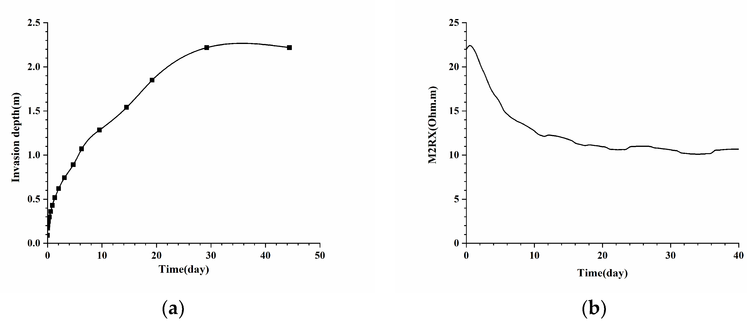
4.2.2. Analysis of Resistivity Response Value

The porosity of the effective reservoir is relatively higher, and the combination of Formula (5) shows that the reconstructed resistivity response should be relatively lower. In fact, due to the existence of fluid in the effective reservoir, the actual resistivity response is usually higher than the result of the reconstructed curve. For ineffective reservoirs, the resistivity of the reconstructed original formation is significantly higher than that of the actual measured deep lateral resistivity, that is, the actual measured deep lateral resistivity is low, which is also the reason why the resistivity box diagram corresponding to Figure 2f cannot distinguish between effective and ineffective reservoirs. This paper discusses this and analyzes and numerically simulates the reason for the phenomenon of “low resistivity”. Firstly, the analysis combined with the clay mineral measurement results found that the clay content of the L block reservoir is low and that smectite and mixed-layer illite is not developed, so it is not easy to form a low-resistance gas layer caused by clay additional conductivity, and the X-ray whole rock mineral diffraction results also showed that the Shiqianfeng Group and Shihezi Group do not contain pyrite, i.e., it is not caused by conductive minerals. By checking the site construction logs, it was found that the logging time was separated from the drilling time by a large margin, with most wells exceeding 20 days. Considering that the drilling fluid will intrude upon the formation, i.e., due to the intrusion of the drilling fluid, the saturation of the formation fluid around the wellbore, the salinity of the water, and the corresponding resistivity profile will be changed so that the electric logging cannot accurately reflect the true resistivity of the formation due to its influence. In this paper, the process of mud filtrate intrusion into the formation can be approximated by the two-phase seepage equation. However, there are three important differences compared with the preconditions of the Beckley–Levelt oil drive theory in seepage mechanics: (1) For low-porosity and low-permeability reservoirs, the influence of gravity and capillary pressure on the intrusion is relatively enhanced during the intrusion of mud filtrate because the intrusion rate is small. (2) The intrusion rate decreases continuously with time, which is unstable Darcy seepage. (3) Since intrusion is a process that continuously advances radially from the borehole to the formation, the intrusion rate per unit area will become smaller as the depth of intrusion continues to increase. Therefore, the two-phase seepage equation is only an approximate description of the intrusion.

$$\frac{1}{r}\frac{\partial }{\partial r}(r\frac{{\rho }_{g}K{K}_{rg}}{{\mu }_g}\frac{\partial P_g}{\partial r})+q_g=\frac{\partial (\Phi {\rho }_g{S}_g)}{\partial t}$$

(12)

$$\frac{1}{r}\frac{\partial }{\partial r}(r\frac{{\rho }_{w}K{K}_{rw}}{{\mu }_w}\frac{\partial P_w}{\partial r})+q_w=\frac{\partial (\Phi {\rho }_w{S}_w)}{\partial t}$$

(13)

In Equations (12) and (13), $r$ is the borehole radius, ${\rho }_{\mathrm{g}}$ and ${\rho }_w$ are the gas and water densities, respectively, $K$ is the permeability, $\mu$ is the viscosity factor, $P$ is the pressure, $S$ corresponds to the saturation, $t$ is the intrusion time, and $P_c=P_g-P_w$,$S_g+S_w=1$.

Mud filtrate replaces the original fluid in the reservoir under a positive pressure difference between the formation and the borehole. When it is an immiscible fluid (e.g., water-driven oil), the replacement process dominates; when it is a compatible fluid, such as a highly mineralized mud filtrate replacing the low-mineralized formation water, there is not only a replacement process but also ion diffusion and convective transport. The mineralization of the formation water can be transformed by the following equation, and then the radial distribution of the resistivity of the formation water in the intrusion zone can be obtained:

$$R_w=\left(0.0123+\frac{3647.5}{C_w{}^{0.955}}\right)\frac{82}{39+1.8T}$$

(14)

In Equation (14), $R_w$ is the formation water resistivity, $C_w$ is the mineralization, and $T$ is the temperature.

The radial distribution variation in the formation water resistivity under mud filtrate intrusion and the characteristics of radial distribution variation in water-bearing saturation can be obtained by numerical simulation and determined by the Archie model (Equation (4)). When the radial distribution of the formation resistivity $R_t$ is derived and when the formation resistivity $R_t$ varies radially, the instrument receives the formation resistivity $R_a$ as

$$\frac{1}{R_a}={\displaystyle {\int }_0^{\infty }\frac{g(r)}{R_t(r)}}dr$$

(15)

In Equation (15), g(r) is the radial differential geometry factor of the coil system.

Figure 10 shows the numerical simulation results of drilling fluid intrusion in section 1467–1473 m of the L3 well with the following simulated parameters: porosity is 12%, permeability is 1.5 × 10⁻³ ${\mathsf{\mu }\mathrm{m}}^2$, formation water mineralization is 49,500 ppm, mud filtrate mineralization is 3400 ppm, formation temperature is 42.98 °C, borehole pressure is 20 MPa, and formation pressure is 14.5 MPa. Figure 10a shows the variation in the pattern of intrusion depth with soaking time; with increasing soaking time, the intrusion depth also increases gradually, and when the soaking time reaches a certain time, i.e., after 30 days of soaking, the intrusion depth no longer changes. Figure 10b shows the response characteristics of the induction resistivity during drilling fluid intrusion, where M2RX represents the deepest detected induced resistivity. It can be seen that the deep lateral resistivity decreases sharply in the first 5 days of drilling fluid immersion and continues to decrease when the drilling fluid is immersed for more than 5 days, and the change in the deep resistivity decreases gradually and stabilizes after 14 days of immersion.

In addition, in this paper, the effect of porosity on drilling fluid intrusion is analyzed. Figure 11 shows the effect of porosity on the response of deep lateral resistivity logging under drilling fluid intrusion conditions (simulation of the variation in the response of M2RX with intrusion time for the porosity of 0.08, 0.12, and 0.16, and the mineralization of drilling fluid is selected as 3400 mg/L, water saturation is 0.3, and permeability is 5 mD). As can be seen from Figure 11, the larger the porosity, the smaller the M2RX logging response at the same time of intrusion when all conditions are consistent, indicating that the larger the pore space, the more mud filtrate is needed to replace the fluid in the original reservoir pore space during the replacement process, which reduces the mud filtrate intrusion rate, leading to a smaller decrease in the M2RX logging response. This explains why the resistivity cannot be distinguished between ineffective and effective reservoirs because the resistivity of the aquifer and the ineffective reservoir affected by the intrusion have overlapping responses. In contrast, the resistivity curves reconstructed via porosity and Archie’s formula using the method outlined in this paper can be effectively characterized.

4.2.3. Error Analysis

The method outlined in this paper also produces some errors in practical application. Taking well L2 as an example (Figure 12), the production conclusion is consistent with the judgment of the method in this paper. For the 1550–1575 m reservoir, the interpretation concluded that the gas and poor gas layers are interspersed with dry layers. The method proposed in this paper can identify the effectiveness of the reservoir for the gas and poor gas layers, but there are errors in the identification of thin layers and mutual layers, which are caused by the logging response being in the “half amplitude point” or the lack of longitudinal resolution of the logging curve. Such errors are usually unavoidable and can be determined by the field experience of the interpreter. In addition, the main sources of error in this paper are the acquisition error of the log response, which is affected by the borehole environment and field construction and usually cannot be avoided; errors in the calculation of porosity are often difficult to avoid. In this paper, the logging response and physical property parameters have been comprehensively considered. Even with the above errors, the validity of the reservoir can be accurately judged.

4.2.4. Limitations

In this section of the paper, the advantages and error sources of reservoir effectiveness identification based on the double-factor method are discussed, and the limitations of this method are also mentioned. (1) This method cannot avoid the influence of reservoir-surrounding rock. At the layer interface, when the effective reservoir and the ineffective reservoir are interbedded, logging curve response distortion or drastic change often occurs, which leads to the inaccurate calculation of the double factors and the occurrence of misjudgment. (2) The selection of logging curves also needs to be determined according to the actual logging response; the research object of this paper is the tight gas reservoir, meaning that, theoretically, the selected natural gamma curve, compensated density curve, and acoustic time difference curve are sensitive to the response of the effective reservoir, taking into account the obvious influence of intrusion on the reservoir; the resistivity logging series is not taken into account in the target block. If the applied block is free of intrusion, and also the response of resistivity logging shows a changing trend in the identification of reservoir effectiveness, then this series can be included in the identification factor $F_1$, i.e., the construction of the identification factor $F_1$ should be decided according to the logging response of the actual work area. (3) The construction process outlined in this paper is effective for different geological backgrounds, but the actual values of effective reservoir determination are not universal and need to be calculated according to the actual data of actual workings and actual layers.

5. Conclusions

In this paper, based on conventional geophysical logging data combined with physical parameters, a reservoir effectiveness identification method based on a double-factor method is proposed. Considering the logging response and calculation parameters of the reservoir, the identification factor $F_1$ can be constructed by using the natural gamma curve, compensation density curve, and acoustic time difference curve, and the identification factor $F_2$ can be constructed by using porosity and Archie’s formula. The effective reservoir can be identified by intersecting the double factors and providing the determination range. The reservoir effectiveness identification factors $F_1$ and $F_2$ achieved good results in the identification of effective reservoirs in the study area. The coincidence rate between the discriminant results and the production or test results reached 96%, which is higher than the accuracy of the porosity and permeability crossplot method and the maximum curvature method of the mercury injection curve in the traditional method. Compared with the direct use of the lower limit of porosity for judgment, the application risk of this method is low, and the calculation is simple and easy to implement. For work areas with different geological backgrounds, the model construction process of this paper can be used to redetermine the scope of determination. In summary, the reservoir effectiveness identification method proposed in this paper lays a solid foundation for subsequent fluid property identification and production calculation.

References

1. Yin, S.; Lv, D.; Ding, W. New Method for Assessing Microfracture Stress Sensitivity in Tight Sandstone Reservoirs Based on Acoustic Experiments. Int. J. Geomech. 2018, 18, 1–16. [Google Scholar] [CrossRef]
2. Liu, B.; Bai, L.; Chi, Y.; Jia, R.; Fu, X.; Yang, L. Geochemical characterization and quantitative evaluation of shale oil reservoir by two-dimensional nuclear magnetic resonance and quantitative grain fluorescence on extract: A case study from the Qingshankou Formation in Southern Songliao Basin, northeast China. Mar. Pet. Geol. 2019, 109, 561–573. [Google Scholar] [CrossRef]
3. Li, Y.; Zhou, D.-H.; Wang, W.-H.; Jiang, T.-X.; Xue, Z.-J. Development of unconventional gas and technologies adopted in China. Energy Geosci. 2020, 1, 55–68. [Google Scholar] [CrossRef]
4. Stow, D.; Nicholson, U.; Kearsey, S.; Tatum, D.; Gardiner, A.; Ghabra, A.; Jaweesh, M. The Pliocene-Recent Euphrates river system: Sediment facies and architecture as an analogue for subsurface reservoirs. Energy Geosci. 2020, 1, 174–193. [Google Scholar] [CrossRef]
5. Yoshida, M.; Santosh, M. Energetics of the Solid Earth: An integrated perspective. Energy Geosci. 2020, 1, 28–35. [Google Scholar] [CrossRef]
6. Zou, C.; Zhu, R.; Liu, K.; Su, L.; Bai, B.; Zhang, X.; Yuan, X.; Wang, J. Tight gas sandstone reservoirs in China: Characteristics and recognition criteria. J. Pet. Sci. Eng. 2012, 88–89, 82–91. [Google Scholar] [CrossRef]
7. Santosh, M.; Feng, Z. New horizons in energy geosciences. Energy Geosci. 2020, 1, A1. [Google Scholar] [CrossRef]
8. Nolte, S.; Fink, R.; Krooss, B.M.; Littke, R. Simultaneous determination of the effective stress coefficients for permeability and volumetric strain on a tight sandstone. J. Nat. Gas Sci. Eng. 2021, 95, 104186. [Google Scholar] [CrossRef]
9. Shi, B.; Chang, X.; Liu, Z.; Liu, Y.; Ge, T.; Zhang, P.; Wang, Y.; Wang, Y.; Mao, L. Physical-property cutoffs of tight reservoirs by field and laboratory experiments: A case study from Chang 6, 8–9 in Ordos Basin. Front. Earth Sci. 2021, 15, 471–489. [Google Scholar] [CrossRef]
10. Qassamipour, M.; Khodapanah, E.; Tabatabaei-Nezhad, S.A. A comprehensive method for determining net pay in exploration/development wells. J. Pet. Sci. Eng. 2020, 196, 107849. [Google Scholar] [CrossRef]
11. Yang, T.; Cao, Y.; Wang, Y.; Liu, K.; He, C.; Zhang, S. Determining permeability cut-off values for net pay study of a low-permeability clastic reservoir: A case study of the Dongying Sag, eastern China. J. Pet. Sci. Eng. 2019, 178, 262–271. [Google Scholar] [CrossRef]
12. Otchere, D.A.; Ganat, T.O.A.; Nta, V.; Brantson, E.T.; Sharma, T. Data analytics and Bayesian Optimised Extreme Gradient Boosting approach to estimate cut-offs from wireline logs for net reservoir and pay classification. Appl. Soft Comput. 2022, 120, 108680. [Google Scholar] [CrossRef]
13. Worthington, P.F. The Application of Cutoffs in Integrated Reservoir Studies. SPE Reserv. Eval. Eng. 2008, 11, 968–975. [Google Scholar] [CrossRef]
14. Masoudi, P.; Arbab, B.; Mohammadrezaei, H. Net pay determination by Dempster rule of combination: Case study on Iranian offshore oil fields. J. Pet. Sci. Eng. 2014, 123, 78–83. [Google Scholar] [CrossRef] [Green Version]
15. Bouffin, N.; Jensen, J. Efficient Detection of Productive Intervals in Oil and Gas Reservoirs. In Proceedings of the Canadian International Petroleum Conference, Calgary, AB, Canada, 16–18 June 2009. [Google Scholar] [CrossRef]
16. Wang, Y.; Cao, Y.; Song, G.; Song, L.; Yang, T.; Zhang, S. Analysis of petrophysical cutoffs of reservoir intervals with production capacity and with accumulation capacity in clastic reservoirs. Pet. Sci. 2014, 11, 211–219. [Google Scholar] [CrossRef] [Green Version]
17. Worthington, P.F.; Cosentino, L. The Role of Cutoffs in Integrated Reservoir Studies. SPE Reserv. Eval. Eng. 2005, 8, 276–290. [Google Scholar] [CrossRef]
18. Egbele, E.; Ezuka, I.; Onyekonwu, M. Net-to-gross ratios: Implications in integrated reservoir management studies. In Proceedings of the Nigeria Annual International Conference and Exhibition, Abuja, Nigeria, 1–3 August 2005. [Google Scholar]
19. Mahbaz, S.; Sardar, H.; Namjouyan, M.; Mirzaahmadian, Y. Optimization of reservoir cut-off parameters: A case study in SW Iran. Pet. Geosci. 2011, 17, 355–363. [Google Scholar] [CrossRef]
20. Harfoushian, J.H.; Suriyanto, O. Net Pay Cutoff Determination Using In-Situ Permeability Measurements with Advanced Formation Testers. In Proceedings of the SPE Asia Pacific Oil & Gas Conference and Exhibition, Perth, Australia, 25–27 October 2016. [Google Scholar] [CrossRef]
21. Masoudi, P.; Tokhmechi, B.; Zahedi, A.; Jafari, M.A. Developing a method for identification of net zones using log data and diffusivity equation. Int. J. Min. Reclam. Environ. 2012, 2, 53–60. [Google Scholar] [CrossRef]
22. Masoudi, P.; Tokhmechi, B.; Jafari, M.A.; Zamanzadeh, S.M.; Sherkati, S. Application of Bayesian in determining productive zones by well log data in oil wells. J. Pet. Sci. Eng. 2012, 94–95, 47–54. [Google Scholar] [CrossRef] [Green Version]
23. Masoudi, P.; Arbab, B.; Mohammadrezaei, H. Net pay determination by artificial neural network: Case study on Iranian offshore oil fields. J. Pet. Sci. Eng. 2014, 123, 72–77. [Google Scholar] [CrossRef] [Green Version]
24. Mehdipour, V.; Ziaee, B.; Motiei, H. Determination and distribution of petro physical parameters (PHIE, Sw and NTG) of Ilam Reservoir in one Iranian oil filed. Life Sci. J. 2013, 10, 153–161. [Google Scholar] [CrossRef]
25. Gao, H.; Li, H. Determination of movable fluid percentage and movable fluid porosity in ultra-low permeability sandstone using nuclear magnetic resonance (NMR) technique. J. Pet. Sci. Eng. 2015, 133, 258–267. [Google Scholar] [CrossRef]
26. Zheng, S.; Yao, Y.; Liu, D.; Cai, Y.; Liu, Y. Characterizations of full-scale pore size distribution, porosity and permeability of coals: A novel methodology by nuclear magnetic resonance and fractal analysis theory. Int. J. Coal Geol. 2018, 196, 148–158. [Google Scholar] [CrossRef]
27. Zhang, S.; Wang, J.; Zhang, Y.; Zhang, X.; Zhang, T.; Cui, J. Determination of petrophysical property cutoffs of lacustrine dolomite intercrystalline pore reservoir in the Xiaganchaigou Formation, western Qaidam Basin. Acta Pet. Sin. 2021, 42, 44–45+118. [Google Scholar] [CrossRef]
28. Yang, Z.; Tang, X.; Xiao, H.; Zhang, F.; Jiang, Z.; Liu, G. Water film thickness of tight reservoir in Fuyu oil layer of Cretaceous Quantou Formation in Songliao Basin and its influence on the lower limit of seepage. Mar. Pet. Geol. 2022, 139, 105592. [Google Scholar] [CrossRef]
29. Qin, B.; Cao, B.; Zhou, J.; Zhang, L.; Lei, Y.; Zhang, Z. Availability identification of tight gas sandstone reservoirs and quantitative assessment: A case study from the first member of the Upper Paleozoic Shanxi Formation in the southeastern Ordos Basin. Acta Sedimentol. Sin. 2019, 37, 403–405. [Google Scholar] [CrossRef]
30. Mi, H.; Zhang, B.; Zhu, G.; Su, Y.; Zhang, H. Geological characteristics and development potential analysis of Linxin tight sandstone gas reservoir. Spec. Oil Gas Reserv. 2022, 29, 65–72. [Google Scholar] [CrossRef]
31. Zhu, G.; Li, B.; Li, Z.; Du, J.; Liu, Y.; Wu, L. Practices and development trend of unconventional natural gas explorationin eastern margin of Ordos Basin: Taking Linxing-Shenfu gas field as an example. China Offshore Oil Gas 2022, 34, 16–29+261. [Google Scholar] [CrossRef]
32. Zhao, J.; Liu, L.; Li, X.; Zhou, G.; Wang, X. Review and forecast of technique research on fluid identification of low and particularly low permeability sandstone reservoir. Prog. Geophys. 2009, 24, 1446–1453. [Google Scholar] [CrossRef]
33. Zhu, L.; Wu, S.; Zhou, X.; Cai, J. Saturation evaluation for fine-grained sediments. Geosci. Front. 2023, 14, 101540. [Google Scholar] [CrossRef]
34. Guo, J.; Ling, Z.; Xu, X.; Zhao, Y.; Yang, C.; Wei, B.; Zhang, Z.; Zhang, C.; Tang, X.; Chen, T.; et al. Saturation Determination and Fluid Identification in Carbonate Rocks Based on Well Logging Data: A Middle Eastern Case Study. Processes 2023, 11, 1282. [Google Scholar] [CrossRef]
35. Archie, G.E. The Electrical Resistivity Log as an Aid in Determining Some Reservoir Characteristics. Trans. AIME 1942, 146, 54–62. [Google Scholar] [CrossRef]
36. Wu, Y.; Hu, X.; Yang, D.; Wu, J.; Yuan, W. A new method of obtaining core irreducible water saturation based on capillary pressure curve. Bull. Geol. Sci. Technol. 2018, 37, 100–105. [Google Scholar] [CrossRef]
Figure 1. Geographical location diagram and lithology histogram of the study area.
Processes 11 02195 g001
Figure 2. Boxplot of logging response for effective and ineffective reservoirs: (a) boxplot of well diameter logging curve response for effective and ineffective reservoirs. (b) Boxplot of compensation neutron logging curve response for effective and ineffective reservoirs. (c) Boxplot of compensating density logging curve response for effective and ineffective reservoirs. (d) Boxplot of acoustic time difference logging curve response for effective and ineffective reservoirs. (e) Boxplot of natural gamma logging curve response for effective and ineffective reservoirs. (f) Boxplot of M2RX logging curve response for effective and ineffective reservoirs. (g) Boxplot of PE logging curve response for effective and ineffective reservoirs. (h) Boxplot of natural potential logging curve response for effective and ineffective reservoirs.
Processes 11 02195 g002aProcesses 11 02195 g002b
Figure 3. Discrimination process of reservoir effectiveness based on the double-factor method.
Processes 11 02195 g003
Figure 4. Crossplot of compensated density logging response and porosity. The dot is the intersection of core porosity and compensated density log response, and the red dashed line is the fitting trend line of both.
Processes 11 02195 g004
Figure 5. Determination of rock and electricity parameters in the study area: (a) intersection of formation factors with porosity to calculate a and the cementation index; (b) intersection of resistance increase coefficient with water saturation to calculate b and saturation index.
Processes 11 02195 g005
Figure 6. Reservoir effectiveness identification chart based on the double-factor method. The vertical blue dashed line is the cutoff value for F1, and the horizontal blue dashed line is the cutoff value for F2.
Processes 11 02195 g006
Figure 7. Effect of applying the double-factor reservoir effectiveness identification method to new wells.
Processes 11 02195 g007
Figure 8. Effect of applying the method outlined in this paper in the L1 well.
Processes 11 02195 g008
Figure 9. The traditional method determines the lower limit of porosity of the target block: (a) the lower limit of porosity is determined by the porosity–permeability crossplot method, the dot is the intersection of core porosity and core permeability, and the red dashed line is the fitting trend line of both, and the blue line is used to indicate the lower porosity limit; (b) the lower limit of porosity is determined by the mercury injection curve method, the dot is the intersection of the median mercury saturation pressure and the core porosity, and the red dashed line is the fitting trend line of both, and the blue line is used to indicate the lower porosity limit.
Processes 11 02195 g009
Figure 10. Numerical simulation results of drilling fluid invasion in 1467–1473 m section of L3 well: (a) the variation of intrusion depth with soaking time; (b) the response characteristics of the induction resistivity during drilling fluid intrusion.
Processes 11 02195 g010
Figure 11. The influence of porosity on deep induction resistivity.
Processes 11 02195 g011
Figure 12. The application effect of this method in the L2 well.
Processes 11 02195 g012