Article

Research of Big Data Production Measurement Method for SRP Wells Based on Electrical Parameters

1
Research Institute of Petroleum Exploration and Development, PetroChina, Beijing 100083, China
2
CNPC Jilin Oilfield Branch CCUS and EOR Development Company, Songyuan 138000, China
*
Author to whom correspondence should be addressed.
Processes 2023, 11(7), 2158; https://doi.org/10.3390/pr11072158
Submission received: 22 May 2023 / Revised: 10 July 2023 / Accepted: 18 July 2023 / Published: 19 July 2023

Abstract

:
Production measurement plays a vital role in the daily management of unconventional oil wells. It enables reservoir managers to gain a comprehensive understanding of reservoir changes and facilitates dynamic analysis and scientific development plans for the unconventional oil field. This paper focuses on accurately measuring well production by tracking over 300 sucker rod pumps (SRPs) in an experimental area of an oil field. The study utilizes easily obtainable continuous electrical parameters and real-time well production as training parameters. Accurate identification of the top and bottom dead points of the power curve is crucial in converting the power curve into the SRP’s dynamometer card. To achieve this, FFT is employed to extract single-period data from multi-period data. Subsequently, the top and bottom dead points are identified. The SRP electric power curve and corresponding real-time production data are segregated into samples based on the stroke cycle time, resulting in 200,000 valid samples. Deep learning techniques are then applied to classify the production state of pumping wells. FFT and statistical feature extraction are performed on the electric curve, and deep learning is utilized with the production parameters as input vectors and the well fluid production as output results. Through extensive training, a big-data-based SRP production calculation model is established, and subsequently used to calculate the production of SRPs in the experimental area of northeastern China’s oil field. The model is validated against actual production data. For low-yield wells with a daily production less than 6 m 3 /d, the model error remains below 0.5 m 3 /d. Additionally, the relative error for high-yield wells surpassing 6 m 3 /d stays under 10%, meeting the expectations of managers. This big data production measurement model serves as a valuable tool for operators to optimize the production system and detect oil well faults. Particularly in a low oil price environment, this method helps managers reduce costs and improve efficiency.

1. Introduction

The main purpose of oil well production measurement is to understand the oil production situation of a single well and provide accurate and reliable data for production management. Oil well production measurement enables managers to grasp the dynamic operation of oil field development, analyze changes in underground oil storage conditions, and formulate reasonable development and adjustment plans. Ultimately, this leads to the improvement of the oil recovery rate, the scientific management of oil fields, and the maximization of development benefits [1,2,3,4].
Oil well production measurement plays a very important role in the production and operation process of unconventional oil fields. Firstly, accurate measurement can obtain production data of oil, gas, and water from a single well. By understanding the crude oil production of oil wells, the dynamic changes in oil well production can be effectively controlled, thereby maintaining the normal order of oil field production operations and management. Secondly, oil well production measurement can guide the formulation and implementation of oil field development strategies and artificial lifting well parameter adjustments, achieving fine management of oil wells. Thirdly, continuous oil well production measurement can help operators detect potential faults in oil wells in a timely manner and take remedial measures earlier.
Oil well production reflects the production level of the oil field comprehensively, and each oil field strives to accurately measure the production of each well. Ideally, each oil well should be equipped with a measurement device for continuous measurement, taking into account only the accuracy of the measurement. However, due to the large number and wide distribution of oil wells, this would require a significant investment, resulting in increased costs of oil and gas products, and is therefore not economically feasible. In order to ensure the economic benefits of oil field development, it is necessary to adopt a simple and economical method for accurate and reliable measurement of oil well production.
As oil field production continues to progress, oil companies have increasingly demanded refined management, and the experimental study and promotion of new measurement technologies have received attention [5,6]. Measurement technology is gradually developing towards equipment miniaturization, high efficiency, continuity, and automation. Researchers have successively carried out research on the working conditions of oil well production systems based on the Gibbs wave equation. With the continuous development of dynamometer diagnostic technology, the working condition changes of each oil well and the changes in instantaneous and cumulative liquid production can be monitored in real time [7,8]. Taking the ground dynamometer of SRPs as the research object, a dynamic coupling model of the rod liquid system of the pumping well is selected, established, and corrected to eliminate the effects of rod deformation, rod viscous damping, and vibration and inertia of the rod and liquid columns contained in the ground dynamometer, and a pump dynamometer is obtained that can truly reflect the working condition of the pump. Based on the working characteristics of the pump dynamometer, a curvature calculation model of the pump dynamometer curve and a calculation model of the effective plunger stroke are established, which can accurately measure the liquid production of oil wells [4,9].

2. Description and Methodology of the System

2.1. Objective and Context

The SRP has always been the main lifting equipment for oil production due to its maturity, wide application, and economic benefits. As the supply capacity of the oil well changes with the production time and the application of stimulation methods, well production measurement is the foundation of oil well production during the oil field production process. For many years, the process of measuring production through the SRP dynamometer card has been relatively mature. This method requires calculating the pump dynamometer card through various parameters, with too many influencing factors resulting in significant errors between the measurement results and actual production, particularly for thick oil wells or high gas–liquid ratio wells, resulting in greater measurement errors. The online continuous automatic and practical measurement of daily liquid production of three-phase flow (oil, gas, and water) at the wellhead of the oil producing well is a worldwide application problem. To reduce the impact of measurement errors on production, the authors have conducted a study on the automated single-well daily liquid production measurement of SRP by selecting easily obtainable continuous electrical parameter data (including electric power, current, and voltage) and real-time well production as training parameters. Through a deep learning model, the electric power curve is converted into a dynamometer card, and the pump efficiency is calculated based on the area of the dynamometer card. Finally, the production is calculated based on the stroke, stroke frequency, and pump diameter. Based on the automatic production calculation device for the pumping unit well electrical parameters, online continuous practical automatic measurement of the single-well daily liquid production of the pumping unit well is realized.

2.2. Description

The power to dynamometer conversion was mainly constructed using a deep learning model. To implement a deep learning algorithm, a network must be constructed, which is also known as a deep learning neural network model. Generally, deep learning can be divided into three steps, as shown in the following Figure 1.
In the first step, the neural network model is a complex function composed of simple functions. Usually, a neural network model (structure) is designed and some parameters are obtained by training from the given training data using a computer, which ensures that the model can achieve the desired effect in the test set and has generalization ability. In the second step, a cost function is defined based on the training data. The cost function can be used to evaluate which parameters are effective and which are not, and which functions in the model are good or not, and how to define a cost function is based on the specific task and actual training data. In the third step, the best function is found based on the results of the previous two steps. For example, the best function can be found using the gradient descent method.

2.3. Method

2.3.1. Device

The hardware equipment of the electric parameter acquisition technology includes the electric parameter acquisition and IoT module of the pumping unit, which is a wellhead-specific collection and communication device customized for the pumping unit. This equipment can realize functions such as real-time electric parameter collection, transmission, and edge intelligent analysis and control at the wellhead of the pumping unit. The hardware design of the equipment is based on an embedded ARM processor, and the overall hardware design architecture consists of a high-precision and high-frequency electric parameter acquisition and calculation module, a high-performance CPU core module, a communication transmission module, and a power supply module. The electric parameter acquisition module consists of voltage–current input module, signal conditioning module, and electric parameter acquisition and calculation module. It completes the collection of electric parameters, including the real-time collection and power calculation of three-phase electric parameters, such as current, voltage, active power, and reactive power. The communication module includes wired communication and wireless communication. Wired communication includes Ethernet communication, RS232/RS485 communication; wireless communication includes 4G/5G communication, WIFI, Zigbee communication, etc. The communication module is responsible for functions such as data transmission and command receiving between the device and mobile phone, back-end server, and supports mobile remote control function, edge local automatic control function, and cloud remote control function. In addition, functions such as online upgrading and time calibration can be completed through the 4G network.
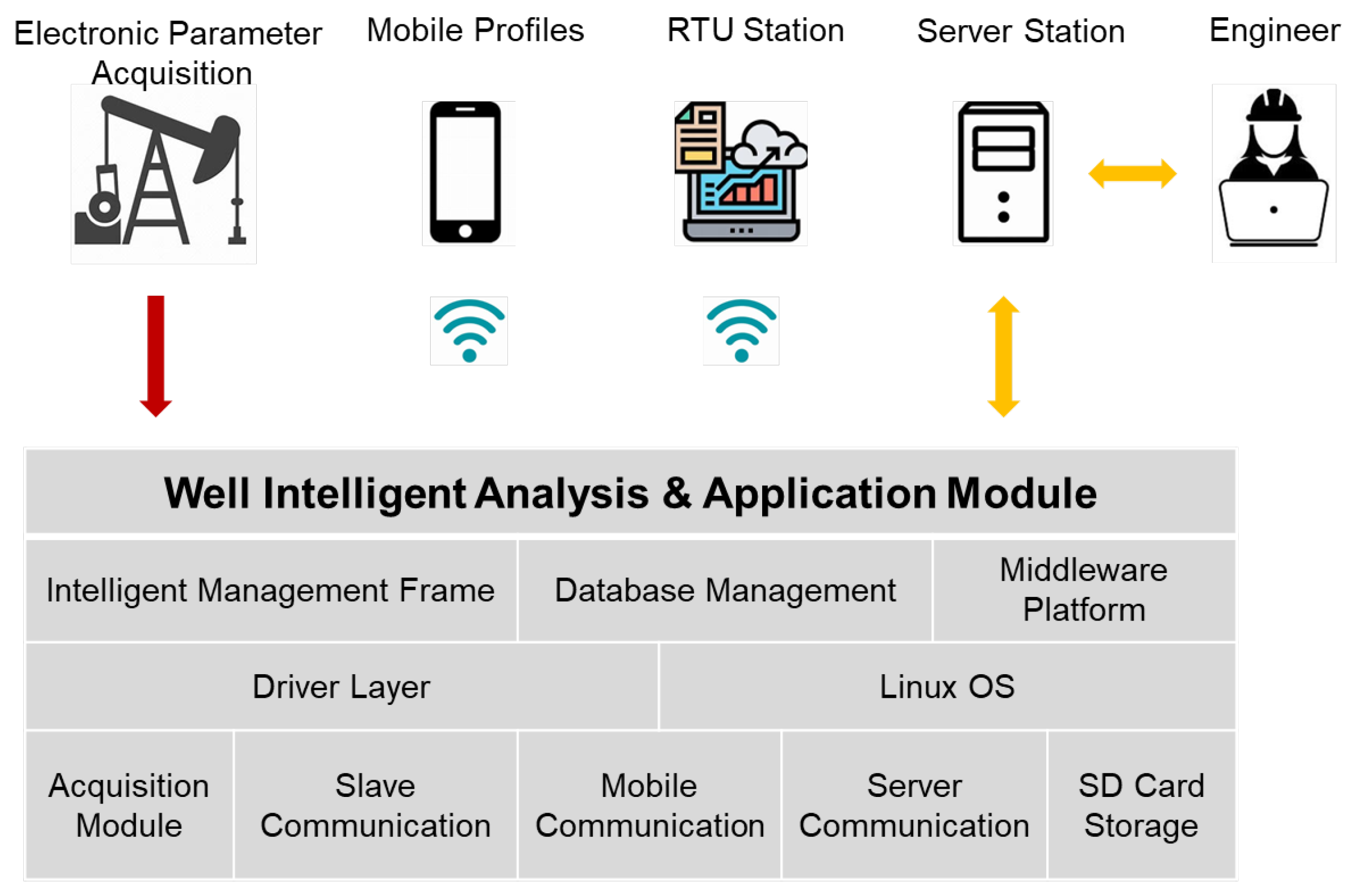
The overall software architecture is based on an embedded Linux operating system and adopts multi-threading technology for program design. It adopts layered design, including hardware layer, driver layer, operating system layer, API interface layer, and application program layer, as shown in the following Figure 2.
The hardware layer is the fundamental module of the hardware system, including electric parameter acquisition, processor, communication, memory storage, and various I/O devices related to hardware chips. It provides basic computational resources and is the foundation on which the operating system and upper-layer software work. The driver layer, also known as Driver, provides external device operation interfaces for upper-layer programs and implements device driver programs. The driver acts as a bridge between the upper-layer application and the lower-layer hardware, providing effective data for the application layer and completing hardware initialization configuration and effective data extraction. The operating system layer mainly completes tasks such as resource scheduling and allocation, information storage and protection, and concurrency coordination and control, providing strong support for system programs such as compiler programs and database management systems. The API layer is the interface layer, providing interface calls required by the application layer for multitasking management, database, communication protocols, etc. The application layer is the specific business layer, mainly including functions such as electric parameter acquisition calculation, data storage, communication transmission, and implementation of communication and control logic with other instrument devices.

2.3.2. Model

The current IoT systems for oil and gas production mainly use two methods to identify the top and bottom dead points of electric parameters and dynamometer card. The first method uses an angle displacement sensor to identify the starting point of the up and down strokes according to the angle of the crankshaft rotation of the pumping unit. The second method collects data synchronously at the same frequency for electric parameters and dynamometer card, where every displacement point has corresponding load and electric parameter data. By identifying the time corresponding to the minimum and maximum displacement points, the bottom dead point and top dead point can be determined, respectively. With the implementation of low-cost IoT construction strategies and the advancement of technologies such as direct diagnosis using electric parameters in the future, identifying the top and bottom dead points of the pumping unit well without angle displacement sensors and dynamometer card will become difficult. On-site oil production engineers can rely on experience to identify the top and bottom dead points by repeatedly observing the changing trends in a large number of electric parameter curves. The method and thought process of identifying the top and bottom dead points by experience provides guidance for us to use machine learning technology for research on dead point identification. Experienced engineers cannot simply judge the top and bottom dead points based on single point electric parameter data, as shown in the following Figure 3, but need to observe the changing trends of previous and subsequent data. As the continuous electric parameters exhibit periodic features, it is only necessary to pay attention to the preliminary changing features of the electric parameter curves for multiple cycles. Therefore, the authors propose to use a big data method to establish an algorithm model for identifying top and bottom dead points based on a large amount of historical data.

Data Preprocessing

The electrical parameters of the SRP generally include the current, voltage, active power, and reactive power at the motor input end. In this paper, the electrical parameters mainly refer to the active power. The electrical parameters are sampled at a certain frequency, and N data points of fixed length are taken in continuous time.
First of all, if the collected data are in hexadecimal format, they need to be converted to decimal. The vector x has a length of N and can be expanded as:
x = [ x 1 , x 2 , , x N ]
Each element x i of the vector x is a decimal real number. During the collection process, due to hardware problems, some abnormal noise points may be generated in the collected data and need to be corrected. For each element x i in the vector x, the value of the element located before x i is denoted as ( x i ), and the value of the element located after x i is denoted as ( x i ). If x i is an abnormal noise point, the following processing is performed on x i :
x i = x i + x i 2

Identifying One Period of Electric Power Curve Using FFT

For preprocessed electrical parameter data, the FFT is used in this paper to extract the frequency domain characteristics. The FFT of a finite-length sequence is defined as follows:
X ( k ) = n = 1 N x ( n ) ( cos 2 π k n N j s i n 2 π k n N )
The real part and the image part are given by:
r e a l X ( k ) = n = 1 N x ( n ) ( cos 2 π k n N )
i m a g X ( k ) = n = 1 N x ( n ) ( sin 2 π k n N )
The square root of the sum of squares of the real part and imaginary part is the spectral feature of the k-th frequency domain.
Fourier transform is applied to the sampled electric power curve to identify the maximum peak and corresponding frequency in the frequency domain. This frequency represents the main period of the electric power curve. If the main period is found to be unreasonable, other possible periods or parameter adjustments are considered for re-calculation. Periodic analysis and oscillation analysis of the electric power curve are performed to obtain more information on the dynamic changes within the well.
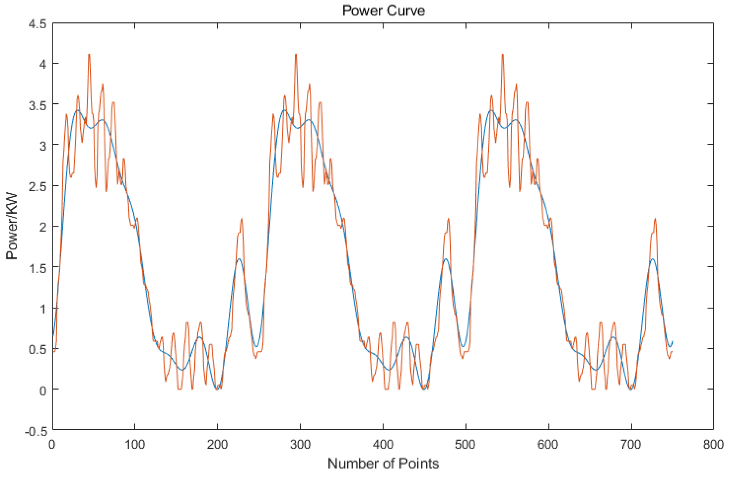
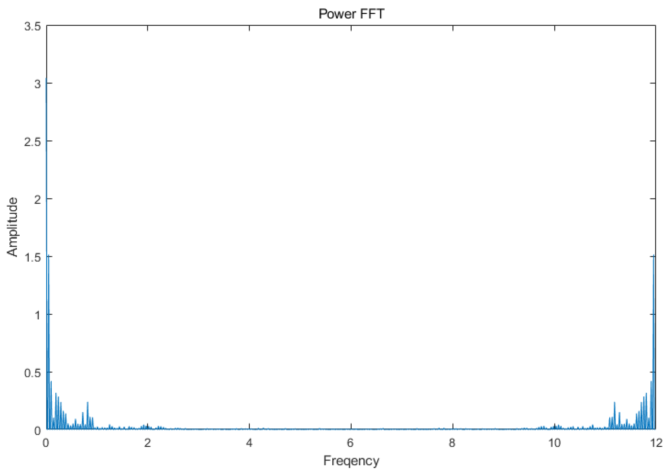
Figure 4 shows the multi-period power curve data obtained from the data acquisition device and the smoothed curve. The periodic data can be transformed into frequency domain representation, as shown in Figure 5, using Fourier transform, and then further processed by filtering and noise reduction methods. In Python, the FFT function in the numpy library can be used for FFT, followed by extracting the single-period signal using symmetry. The specific steps are as follows:
  • Read in the electric power curve data of the oil pumping well and perform FFT operation on each set of data;
  • Extract single cycle signals from the computed FFT results based on symmetry;
  • Perform Inverse Fourier Transformation (IFFT) on the extracted single cycle signals to obtain a periodic curve.
The resulting power curve after single cycle extraction is shown in Figure 6, which consists of 250 test points representing a complete operational cycle of the oil pumping well.
After obtaining the single cycle power curve, the dead center positions can be well reflected by the dynamometer card. The position of the top and bottom dead points on the power curve can be determined by moving and comparing the power curve with the unfolded dynamometer card curve.

Oil Well Production Forecasting Model

Recurrent Neural Networks (RNN) are a type of neural network specifically designed for processing sequential data [10]. RNN can retain the order of the sequence. Long Short-Term Memory (LSTM) is a popular type of RNN. The LSTM network is also a type of recurrent neural network that can solve many tasks that previous recurrent neural network learning algorithms could not solve. The LSTM network introduced gate units, which make use of selective memory and forgetting information, effectively solving the problem of gradient explosion or disappearance. The role of the forget gate is to “forget” information [11,12,13]. In the use of LSTM, some information is not necessary, so the forget gate is used to select these pieces of information and “forget” them. The forget gate decides which information in the memory cell will be forgotten. The role of the memory gate is opposite to that of the forget gate. It determines which information of the new input and the current memory cell will be retained [14,15,16,17]. The LSTM relevant calculation formula is as follows:
f t = s i g m o i d ( W f [ h t 1 , x t ] + b f )
i t = s i g m o i d ( W i [ h t 1 , x t ] + b i )
o t = s i g m o i d ( W o [ h t 1 , x t ] + b o )
c t = f t c t 1 + i t t a n h ( W c [ h t 1 , x t + b c ] )
h t = o t t a n h ( c t )
in which, i, f, and o, respectively, represent the input gate, forget gate, and output gate. W i , W f , W o , and W c are weight matrices, b i , b f , b o , and b c are bias vectors, ⊙ represents element-wise multiplication of matrices, sigmoid is the activation function, and its output range is (0, 1). The calculation process of LSTM network is as follows: (a) Using the external state of the previous LSTM unit h t 1 and the current input x t , calculate the three gate states i t , f t , o t , and the intermediate state C t ˜ ; (b) combine the forget gate f t and the input gate i t to update the memory cell C t ˜ ; (c) combine the output gate o t to transfer the internal state information to the external state h t .
Through our research, it has been found that the Fourier-transformed frequency domain features are feasible. Since electrical power is a sequence data, a transformation can be directly performed on the data of N points. It should be noted that the length of sequence data must be fixed. If it is not fixed, it needs to be converted into fixed N-point power data through interpolation or sampling methods. The amplitude value of DC component should be retained in frequency domain features, while the DC component should be removed for power diagram diagnosis.
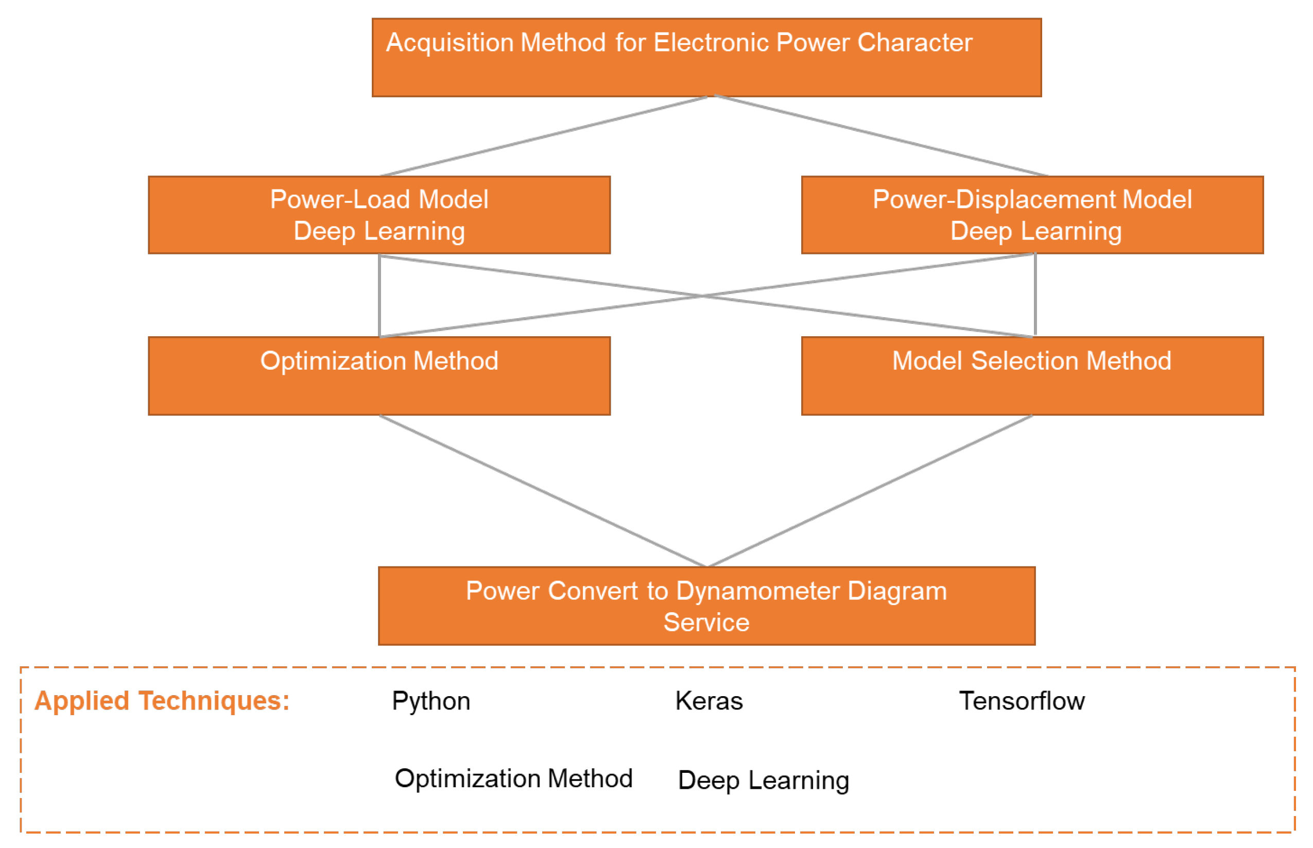
The conversion of electrical power to dynamometer card requires two paths, which involve converting electrical power to the load of the pump rod and converting electrical power to the displacement of the pump rod, and then, matching the load and displacement to obtain the final dynamometer card. Similarly, suitable optimization and model selection methods need to be studied for model training. Finally, these two models need to be embedded into a conversion service to provide a program for converting electrical power to dynamometer card, as shown in Figure 7.
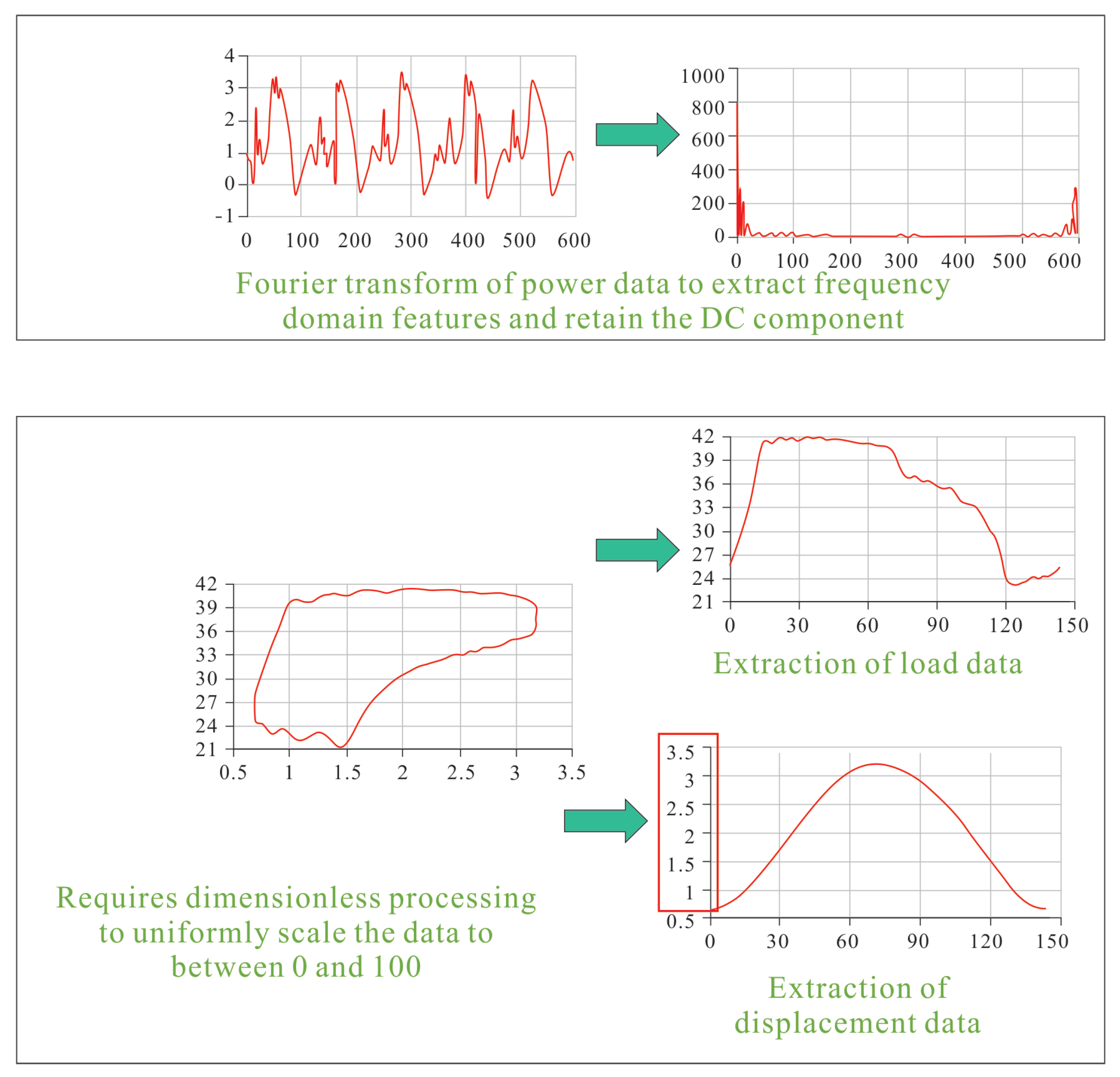
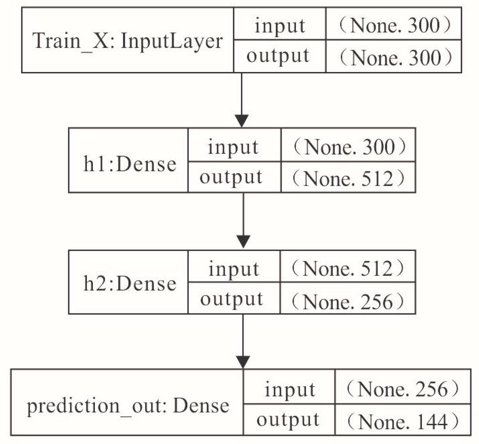
Firstly, the power samples and dynamometer card samples need to be processed separately. The sample processing program converts the power samples into input data samples with frequency domain features after Fourier transform, and splits the dynamometer card samples into load and displacement parts, keeping the same length, which serve as two outputs of the trainer. The power frequency domain features and load are sent to the power-load deep learning trainer as input and output to obtain the power-load predictor. The power frequency domain features and displacement are sent to the power-displacement deep learning trainer as input and output to obtain the power-displacement predictor. The two trainers are used to convert electrical power through the web service. After the electrical power is transmitted from the front end, feature extraction is performed, and then the load and displacement transformations are performed separately using the two trainers, finally synthesizing the dynamometer card, as shown in Figure 8.
The conversion of electrical power to dynamometer card includes four main parts. The electrical power to dynamometer card sample processing function processes the collected electrical power–dynamometer card samples. For example, some electrical power and dynamometer card samples were not collected at the same time, and pairing processing is needed in time to create the samples. The electrical power feature extraction function is used to perform Fourier transform on power data, take frequency domain features, and retain the DC component part, as shown in Figure 9. The electrical power to dynamometer card uses a deep learning model and requires the design of trainers. After obtaining well-trained models, to provide online dynamometer card conversion function on the web, a web service needs to be designed. The Flask architecture microservice is used, and data transmission is performed using JSON. The electrical power to dynamometer card uses two trainers, one to convert electrical power to dynamometer card load and the other to convert electrical power to displacement, as shown in Figure 10. After merging the results predicted by the two trainers, the complete dynamometer card is obtained.
The electrical power calculation model calculates pump efficiency using the area of the dynamometer card obtained by the above power to dynamometer card conversion, and then calculates production based on stroke, stroke frequency, and pump diameter.
Q t h = 1440 S p N A
Subsequently, the daily production of liquid on the surface is calculated based on the volume coefficient B of the crude oil in the well. The production density ρ is obtained by calculating the fluid density of the extracted liquid based on the water content, crude oil density, and water density. Thus, the final daily production of liquid can be determined.
Q = Q t h B ρ

3. Field Application and Analysis

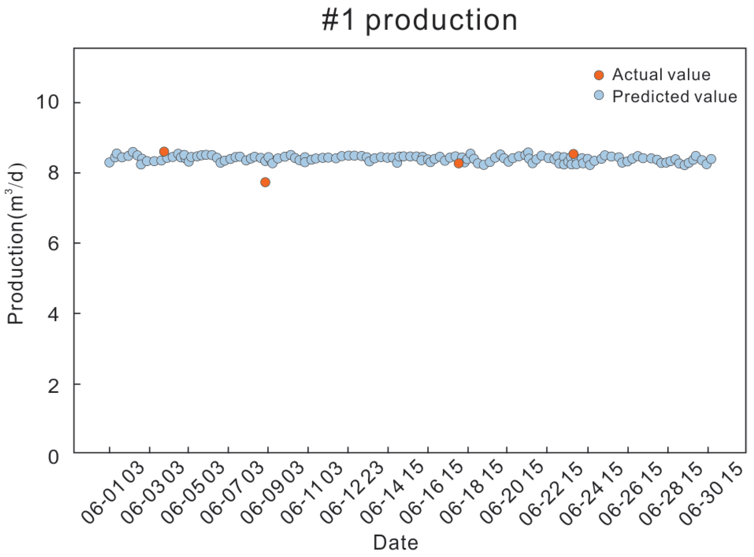
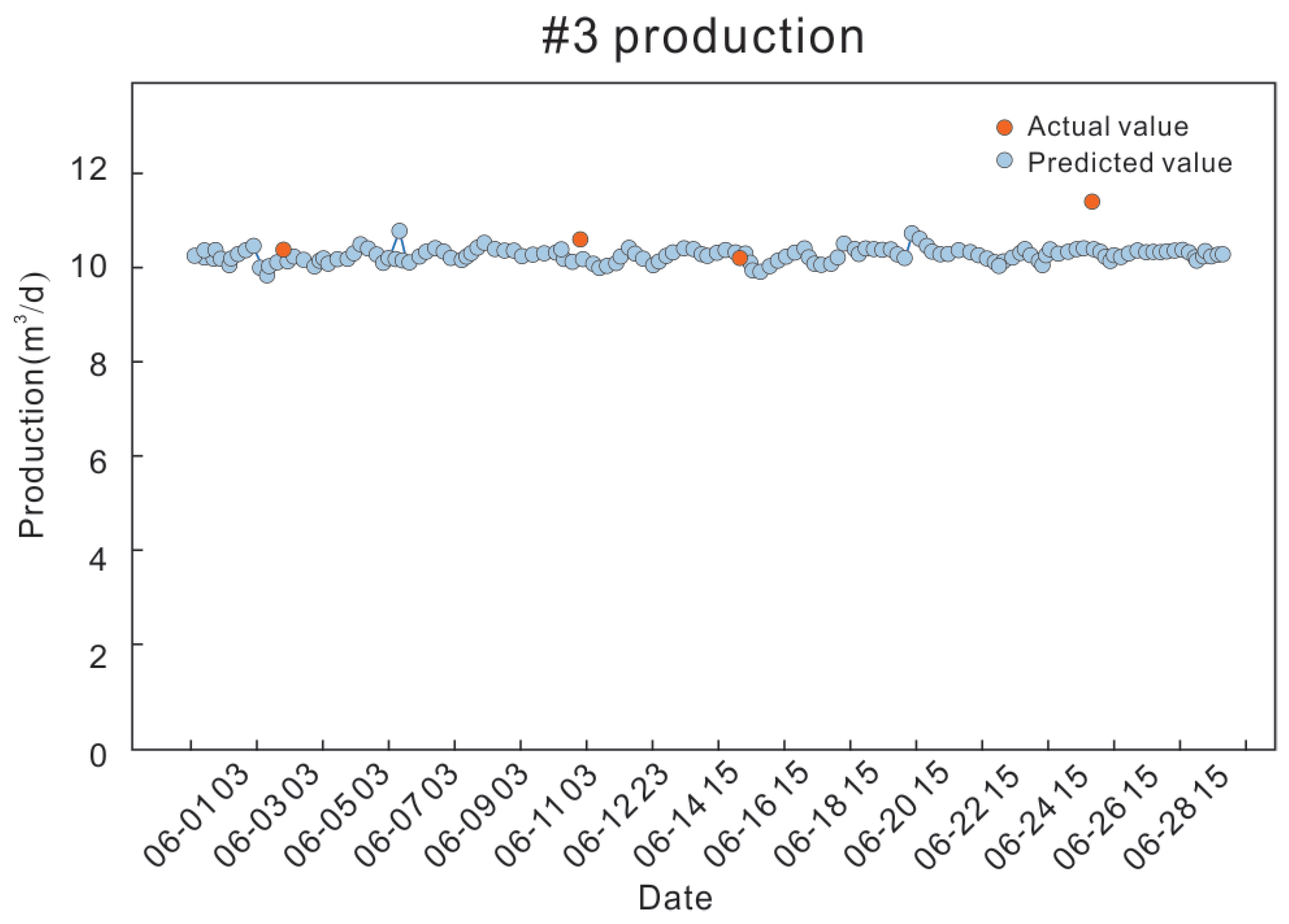
The workflow and model presented in this paper were applied to validate the 332 wells in a block. This block serves as a digital production test area for oil fields, and all wells were installed with electrical parameter acquisition and transmission hardware devices previously. In this study, the model was trained on all production data from the wells within a year, and further validated using 48,398 data points obtained in June 2022. It should be noted that the 332 wells used in the experiment are located within the same block and belong to the same reservoir. The physical property parameters such as crude oil density, viscosity, WOC, etc., are similar. The individual well production is relatively low within the block, and some wells adopt intermittent pumping production methods. Regarding the data collection protocol, electric power and dynamometer card data are collected every 30 min, while daily production rates are measured once a day for sampling purposes. The proposed workflow method calculated the production change curve of each well in the past month, and the production change trend was consistent with the directly measured values. (Note: The block initially used rough measurement by metering multiple wells with a bucket before splitting production.) This section presents some examples of wells with different production levels.
In the examples of wells with stable production, production data from three wells within a month were validated, as shown in Figure 11, Figure 12 and Figure 13, in which the blue dots represent predicted production values using power curves, and the red dots represent actual measured production as the validation data.
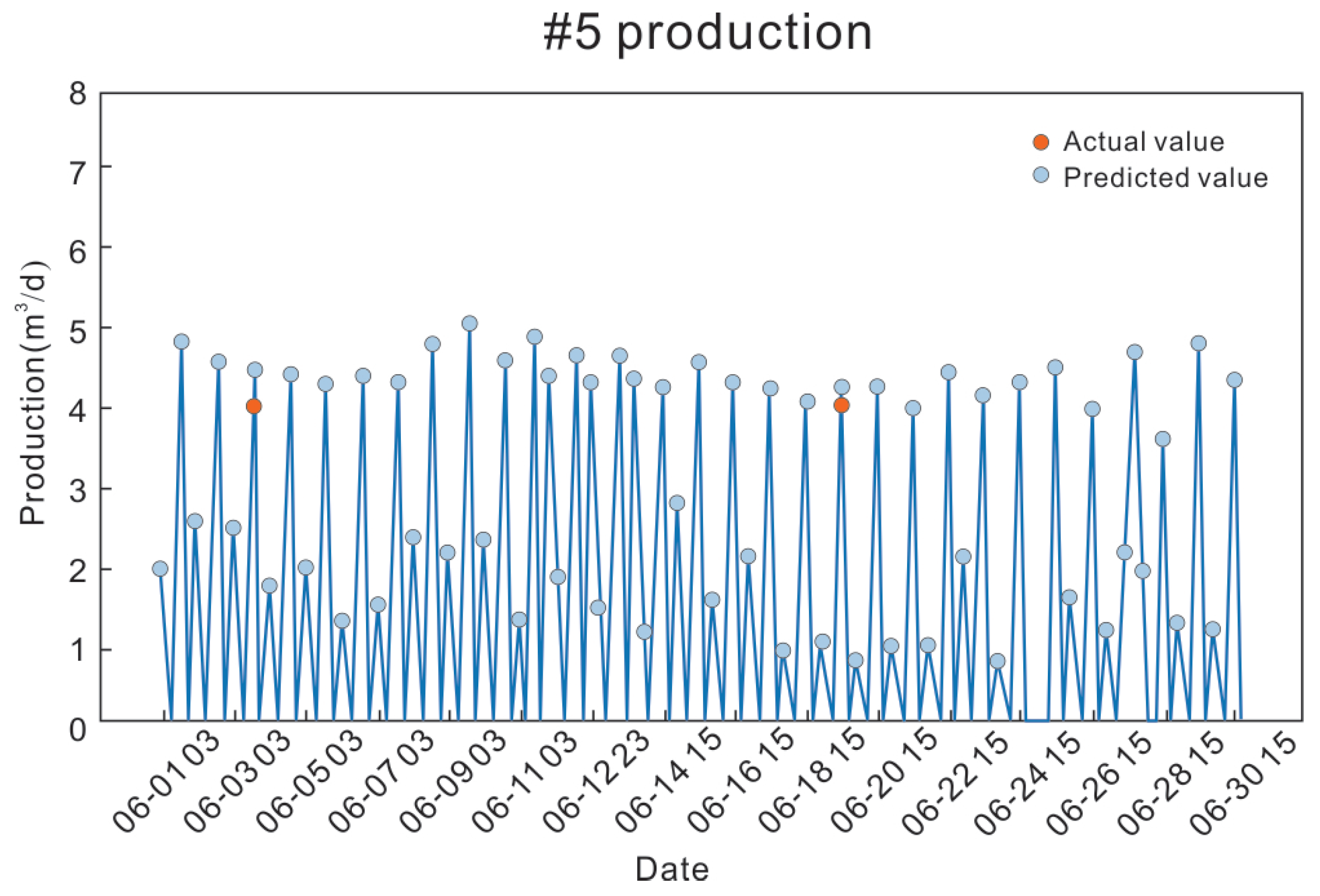
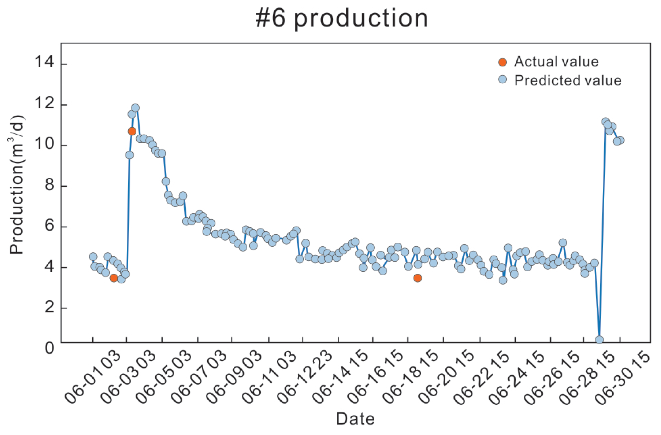
In the examples of intermittent pumping wells, as the production of these wells is low and cannot maintain continuous liquid output, the wells need to be regularly shut down and re-started during production to prevent pump failure and ensure economic benefits. Production data from three intermittent pumping wells within a month were validated, and the model accurately captured the changes in production, as shown in Figure 14, Figure 15 and Figure 16.
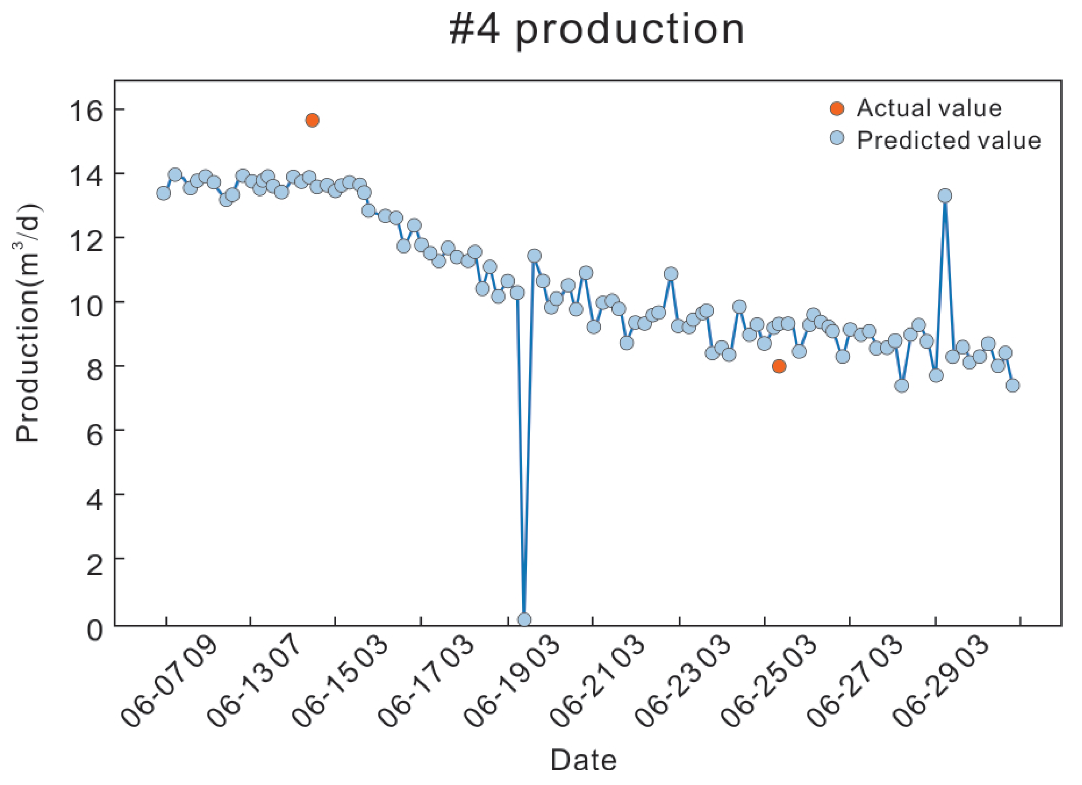
In the examples of wells with unstable production, the production of each well increased or decreased significantly, and the model was able to capture the trend of continuously increasing or decreasing production. Moreover, after conducting well stimulation operations, the model was able to predict a significant increase in production in a timely manner, as shown in Figure 17, Figure 18 and Figure 19.
A comparison and validation of two production measurement methods were randomly selected from the 332 wells in the block. The comparison results are shown in Table 1.
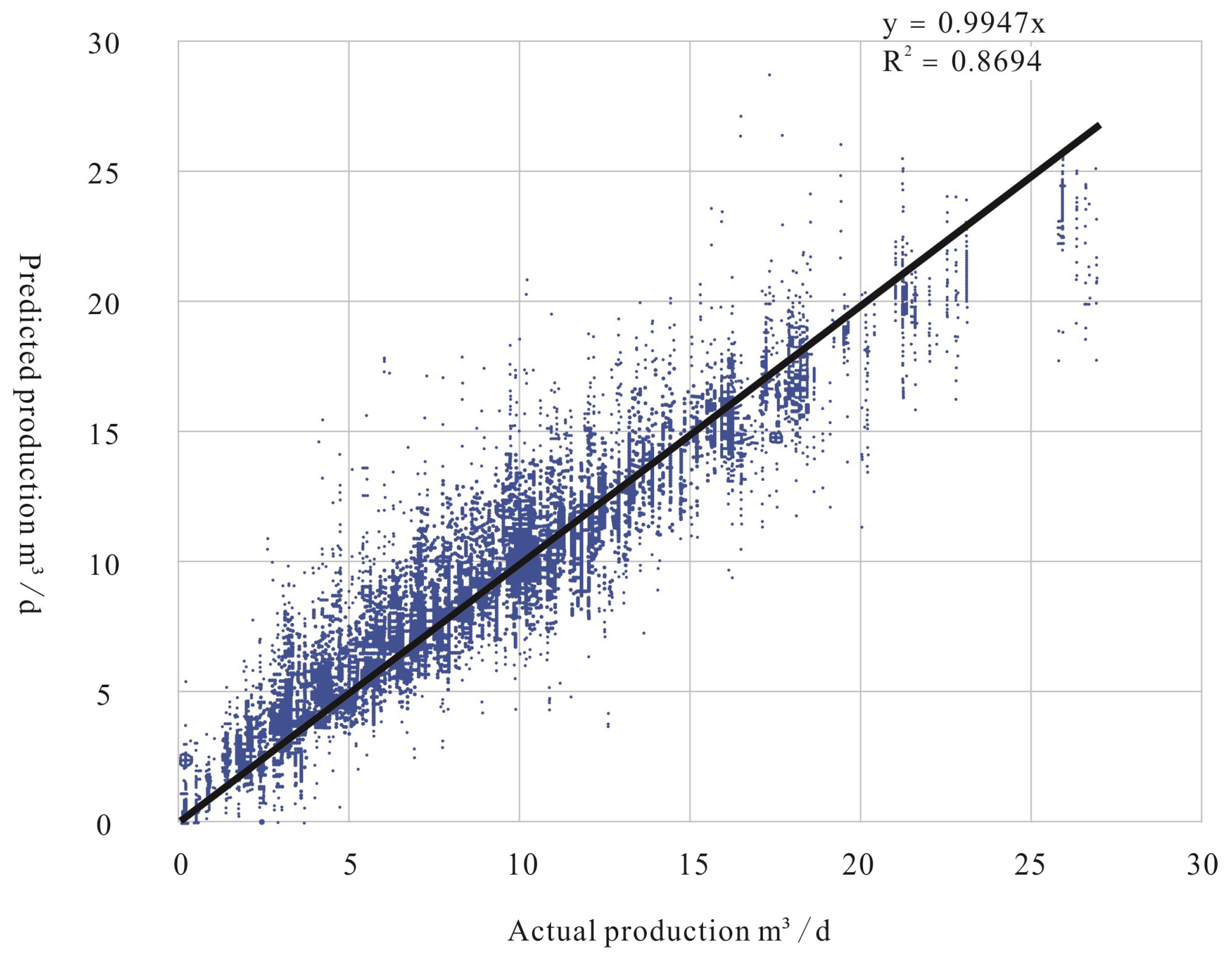
From the single-well prediction curve and validation data table, it can be observed that the model’s predictions have a higher data density compared to the existing tipping bucket metering results and can provide real-time tracking of the production status of oil wells. The relative error of tipping bucket metering is generally considered to be around 15–20%. Since the model predicts the dynamometer card of the oil well, its accuracy can reach 95%. Subsequently, the actual production is calculated using theoretical formulas, and the measurement accuracy is sufficient to meet the requirements of operators. The correlation curve between actual production and predicted production is shown in Figure 20, indicating a high correlation between the model’s predictions and tipping bucket metering results.
Finally, the total production error statistics are shown in Table 2, and the accuracy reached the requirements expected by the oil well managers in this block.
In the process of using LSTM models to predict oil well production, there may be some challenges that could affect the model’s accuracy or impose limitations on its usage. As mentioned earlier, for feature extraction, the dynamometer card data are decomposed into load curve and displacement curve components, from which both time domain and frequency domain information can be obtained. This approach enables the information relevant to electrical power data to be captured effectively. Furthermore, when using oil well electrical power data and dynamometer cards for prediction, it is important to ensure the quality of these data and perform necessary data cleansing and preprocessing. Accurate, complete, and reliable data are crucial for building effective prediction models. The timeframe of the data should also be considered. The performance of the prediction model is often constrained by the available historical data volume and the time range. If there are limited data available or the time range is insufficient to capture the full dynamics of production changes, the accuracy of the model may be affected. To enhance the model’s generalizability for long-term application in other blocks, it is beneficial to generate new training samples by applying transformations such as rotation, translation, scaling, etc., to the original data. This augmentation technique expands the data volume and helps the model learn a greater variety of features and patterns.

4. Conclusions

This article focuses on the research and application results of using oil well electrical parameter data and deep learning methods for flow metering of oil production. The on-site verification results confirm the potential of this process as a production measurement method. However, there are still some deficiencies in the effectiveness of the model for some wells during long-term operation. Therefore, in terms of the model, regular use of measuring instruments is required to assist the model in continuous correction to ensure the accuracy of the entire measurement process.
A deep learning method is proposed to convert the pump well power curve into a dynamometer card. This method is based on feature extraction in the frequency domain after Fourier transform, and achieves learning of the pump rod displacement and load. Accurate identification of up and down dead spots on the power curve can improve the accuracy of production calculation. For wells in different production ranges, this method has a specific range of precision.

Author Contributions

Conceptualization, S.C. and R.Z.; methodology, S.C. and J.S.; software, S.C. and X.Z.; validation, F.D., G.C., H.H. and D.Z.; writing—original draft preparation, S.C.; writing—review and editing, S.C. and F.D. All authors have read and agreed to the published version of the manuscript.

Funding

This research received no external funding.

Institutional Review Board Statement

Not applicable.

Informed Consent Statement

Not applicable.

Data Availability Statement

Not applicable.

Conflicts of Interest

The authors declare no conflict of interest.

Abbreviations

The following abbreviations are used in this manuscript:
SRPSucker rod pump
FTTFast Fourier Transform
IFTTInverse Fast Fourier transform
RNNRecurrent Neural Network
LSTMLong Short-Term Memory

References

  1. Zheng, B.; Gao, X. Diagnosis of Sucker Rod Pumping Based on Dynamometer Card Decomposition and Hidden Markov Model. Trans. Inst. Meas. Control 2018, 40, 4309–4320. [Google Scholar] [CrossRef]
  2. Zheng, B.; Gao, X. Sucker rod pumping diagnosis using valve working position and parameter optimal continuous hidden Markov model. J. Process Control 2017, 59, 1–12. [Google Scholar] [CrossRef]
  3. Kun, L.; Ying, H.; Tong, W. A novel prediction method for down-hole working conditions of the beam pumping unit based on 8-directions chain codes and online sequential extreme learning machine. J. Pet. Sci. Eng. 2017, 59, 285–301. [Google Scholar]
  4. Tao, R.; Xiaoqing, K.; Wen, S.; Hong, S. Study of Dynamometer Cards Identification Based on Root-Mean-Square Error Algorithm. Int. J. Pattern Recognit. Artif. Intell. 2018, 32, 1850004. [Google Scholar]
  5. Peng, X.; Shijin, X.; Yin, H. Application of self-organizing competitive neural network in fault diagnosis of suck rod pumping system. J. Pet. Sci. Eng. 2007, 58, 43–48. [Google Scholar]
  6. Wilamowski, B.; Kaynak, O. Oil well diagnosis by sensing terminal characteristics of the induction motor. IEEE Trans. Ind. Electron. 2000, 47, 1100–1107. [Google Scholar] [CrossRef]
  7. Bezerra, M.A.D.; Schnitman, L.; Filho, M.A.B.; Souza, J.F.D. Pattern Recognition for Downhole Dynamometer Card in Oil Rod Pump System using Artificial Neural Networks. Int. Conf. Enterp. Inf. Syst. 2009, 2, 351–355. [Google Scholar]
  8. Xiao, W.; Rui, Z.; Zhang, H.; Tao, Z.; Su, L. Key Technologies of Sucker Rod Pump Card Diagnosis Based on BP Neural Network. Adv. Mater. Res. 2011, 201–203, 433–437. [Google Scholar]
  9. Zhang, A.; Gao, X. Fault Diagnosis of Sucker Rod Pumping Systems Based on Curvelet Transform and Sparsemulti-graph Regularized Extreme Learning Machine. Comput. Intell. Syst. 2018, 11, 428–437. [Google Scholar] [CrossRef] [Green Version]
  10. Graves, A. Supervised Sequence Labelling with Recurrent Neural Networks. Stud. Comput. Intell. 2012, 385, 1–131. [Google Scholar]
  11. Yu, Y.; Si, X.; Hu, C.; Zhang, J. A Review of Recurrent Neural Networks: LSTM Cells Network Architectures. Neural. Comput. 2019, 31, 1235–1270. [Google Scholar] [CrossRef] [PubMed]
  12. Chen, S.; Ge, L. Exploring the Attention Mechanism in LSTM-based Hong Kong Stock Price Movement Prediction. Quant. Financ. 2019, 19, 1507–1515. [Google Scholar] [CrossRef]
  13. Smagulova, K.; James, A.P. A Survey on LSTM Memristive Neural network Architectures and Applications. Eur. Phys. J. 2019, 228, 2313–2324. [Google Scholar] [CrossRef]
  14. Jonathan, W.; Ying, X. Radically Simplifying Gated Recurrent Architectures Without Loss of Performance. In Proceedings of the 2019 IEEE International Conference on Big Data (Big Data), Los Angeles, CA, USA, 9–12 December 2019; pp. 2615–2623. [Google Scholar]
  15. Greff, K.; Srivastava, R.K.; Koutník, J.; Steunebrink, B.R.; Schmidhuber, J. LSTM: A Search Space Odyssey. IEEE Trans. Neural Netw. Learn. Syst. 2015, 28, 2222–2232. [Google Scholar] [CrossRef] [PubMed] [Green Version]
  16. Federico, L.; Baraldi, L.; Marcella, C.; Cucchiara, R. Working Memory Connections for LSTM. Neural Netw. Off. J. Int. Neural Netw. Soc. 2021, 144, 334–341. [Google Scholar]
  17. Sahin, S.O.; Kozat, S.S. Nonuniformly Sampled Data Processing Using LSTM Networks. IEEE Trans. Neural Netw. Learn. Syst. 2019, 30, 1452–1461. [Google Scholar] [CrossRef] [PubMed] [Green Version]
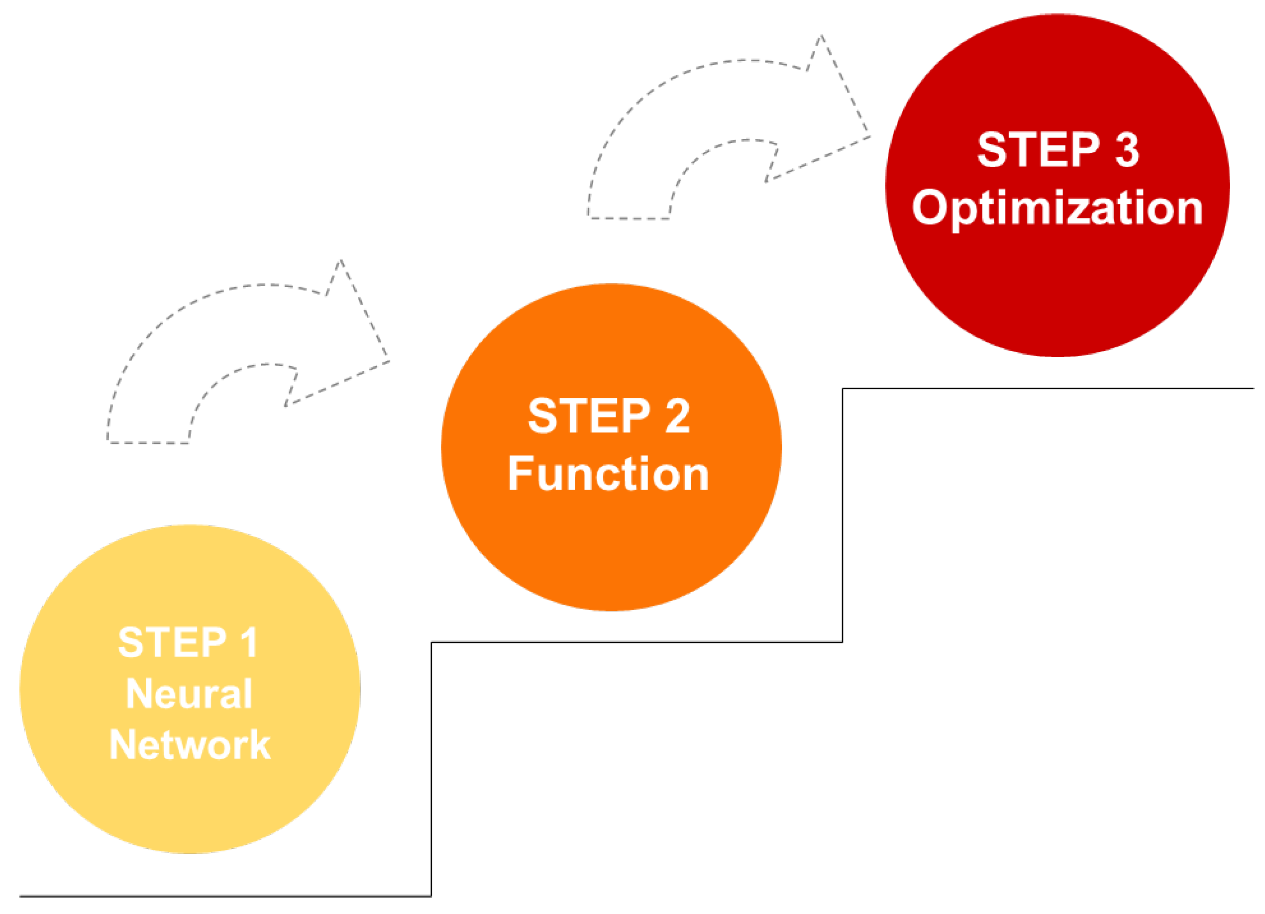
Figure 1. Steps of deep learning. The neural network model is a complex function composed of simple functions. A cost function is defined based on the training data. The best function is found based on the results of the previous two steps.
Processes 11 02158 g001
Figure 2. System software frame.
Processes 11 02158 g002
Figure 3. Electrical parameter curve (one cycle)—it is difficult to identify the top and bottom dead points from the curve.
Processes 11 02158 g003
Figure 4. Multi-period power curve data of an SRP. Multi-period power curve data obtained through data acquisition equipment. Trend of the multi-period power curve after smoothing treatment.
Processes 11 02158 g004
Figure 5. Frequency domain analysis of multi-period power.
Processes 11 02158 g005
Figure 6. The extracted single−cycle power curve by algorithm. The blue line represents data of single−cycle power curve. The orange line represents trend of the single-cycle power curve after smoothing treatment.
Processes 11 02158 g006
Figure 7. The conversion of power curve to dynamometer diagram.
Processes 11 02158 g007
Figure 8. Specific processing flow of electric power to dynamometer diagram.
Processes 11 02158 g008
Figure 9. Technical implementation of electric power conversion.
Processes 11 02158 g009
Figure 10. Establishment of deep learning conversion model.
Processes 11 02158 g010
Figure 11. Sample well #1 with stable production (the vertical coordinate represents the flow rate (m3/d), and the horizontal coordinate represents the date (06- 01 03 represents data No. 3 of 1 June)).
Processes 11 02158 g011
Figure 12. Sample well #2 with stable production (the vertical coordinate represents the flow rate (m3/d), and the horizontal coordinate represents the date (06- 01 03 represents data No.3 of 1 June)).
Processes 11 02158 g012
Figure 13. Sample well #3 with stable production (the vertical coordinate represents the flow rate (m3/d), and the horizontal coordinate represents the date (06- 01 03 represents data No. 3 of 1 June)).
Processes 11 02158 g013
Figure 14. Sample of intermittent pumping well #4 (the vertical coordinate represents the flow rate (m3/d), and the horizontal coordinate represents the date (06- 01 03 represents data No. 3 of 1 June)).
Processes 11 02158 g014
Figure 15. Sample of intermittent pumping well #5 (the vertical coordinate represents the flow rate (m3/d), and the horizontal coordinate represents the date (06- 01 03 represents data No. 3 of 1 June)).
Processes 11 02158 g015
Figure 16. Sample of intermittent pumping well #6 (the vertical coordinate represents the flow rate (m3/d), and the horizontal coordinate represents the date (06- 01 03 represents data No. 3 of 1 June)).
Processes 11 02158 g016
Figure 17. Sample of erratic production well (the vertical coordinate represents the flow rate (m3/d), and the horizontal coordinate represents the date (06- 07 09 represents data No. 9 of 7 June)).
Processes 11 02158 g017
Figure 18. Sample of erratic production well (the vertical coordinate represents the flow rate (m3/d), and the horizontal coordinate represents the date (06- 01 03 represents data No. 3 of 1 June)).
Processes 11 02158 g018
Figure 19. Sample of erratic production well (the vertical coordinate represents the flow rate (m3/d), and the horizontal coordinate represents the date (06- 01 03 represents data No. 3 of 1 June)).
Processes 11 02158 g019
Figure 20. The correlation curve between the actual and predicted production. The blue dots represent data points, and the black line represents the trend line.
Processes 11 02158 g020
Table 1. Comparison results.
Well No.Actual Production m 3 /dPredicted Production m 3 /dAbsolute Error m 3 /dRelative Error
015.65.0004460.59955410.71%
029.58.4134091.08659111.44%
035.64.7422680.85773215.32%
045.65.6317340.0317340.57%
053.43.7685180.36851810.84%
063.43.3850020.0149980.44%
078.87.4850691.31493114.94%
083.43.8980630.49806314.56%
094.85.269420.469429.78%
106.25.389120.9305815.01%
115.66.471080.8710815.56%
127.25.6746761.52532421.96%
Table 2. Statistical results of production.
Total NumberLess than (Equal to) 4 m 3 /d4 m 3 /d to 10 m 3 /d (Equal to)More than 10 m 3 /d
Well time1599297904398
Average absolute error0.850.540.841.12
Average relative error13.67%20.57%13.84%8.14%
Expected standard-Absolute error < 0.6 m 3 /dRelative error < 15 m 3 /dRelative error < 10 m 3 /d
Disclaimer/Publisher’s Note: The statements, opinions and data contained in all publications are solely those of the individual author(s) and contributor(s) and not of MDPI and/or the editor(s). MDPI and/or the editor(s) disclaim responsibility for any injury to people or property resulting from any ideas, methods, instructions or products referred to in the content.