Intelligent Analysis of Vibration Faults in Hydroelectric Generating Units Based on Empirical Mode Decomposition

Abstract

Implementing intelligent identification of faults in hydroelectric units helps in the timely detection of faults and taking measures to minimize economic losses. Therefore, improving the accuracy of fault signal recognition has always been a research focus. This study is based on the improved empirical mode decomposition (EMD) theory to study the denoising and feature extraction of vibration signals of hydroelectric units and uses the backpropagation neural network (BPNN) to establish corresponding connections between signal features and vibration fault states. The improved EMD in this study can improve the performance of noise reduction processing and contribute to the accurate identification of vibration faults. The vibration fault identification criteria can adopt three dimensionless feature parameters: peak skewness coefficient, valley skewness coefficient, and kurtosis coefficient of the second- and third-order components of the signal, with recognition rates and accuracy reaching 90.6% and 96.2%, respectively. This paper’s area under the curve (AUC) values were 0.7365, 0.7335, 0.9232, and 0.9141 for abnormal sound detection of the fan, water pump, slide, and valve, respectively, with an average AUC value of 0.8268. This paper’s accuracy is 90.1%, and the loss function value is 0.27. The validation results demonstrate that this paper’s method has high intelligent fault analysis capabilities. The experimental results confirm that this method can effectively detect vibration signals in hydroelectric units and perform effective noise reduction processing, thereby improving the diagnostic accuracy of fault signals. Therefore, this method can be effectively applied to the detection of vibration faults in hydroelectric units.

1. Introduction

The progress and development of various industries in China cannot be separated from the supply of electricity. Hydroelectric power generation is the second largest power generation method in China, and it has always received high attention from national and local governments due to its low cost and clean environmental protection characteristics [1]. Hydroelectric units are the core components of hydraulic discovery, and their operating status directly affects the power supply of hydropower stations [2,3]. Therefore, achieving intelligent diagnosis and identification of hydroelectric unit faults will help reduce the losses caused by operational faults. The main method for intelligent fault diagnosis and identification of hydroelectric units at present is to identify the overall operation of hydroelectric units using the characteristics of motor frequency signals [4]. According to relevant statistical research, most faults in hydroelectric units can be reflected through the vibration signals of the units. Therefore, the vibration signals and their monitoring in hydroelectric units have important practical significance for the diagnosis of obstacles in hydroelectric units [5]. However, in the current intelligent diagnosis and recognition methods, the presence of noise signals greatly affects the accuracy of fault diagnosis. Given that signal acquisition is often affected by numerous noise signals, this study introduces empirical modal component theory to conduct research and analysis on signal denoising and feature extraction. The research further adopts the backpropagation neural network (BPNN) to establish corresponding recognition relationships between signal feature parameters and motor operation faults, to improve the accuracy of intelligent diagnosis and recognition of fault signals. The article is divided into the following parts: Firstly, the introduction section introduces the background of the article. Then, there is a literature review, which analyzes the current status of the research objects and methods in the article. The following section is a specific explanation of the methods used in the article. The fourth part is the simulation analysis of the method. The fifth part is the conclusion.

2. Related Works

Mechanical fault diagnosis methods can be achieved through the establishment of intelligent methods such as neural networks [6,7,8,9]. Fault diagnosis of high-speed trains is an important measure to ensure the safety of passengers and staff. When establishing fault diagnosis methods for high-speed trains, researchers utilized a hybrid diagnostic model for environmental analysis and data supplementation. This hybrid diagnostic method can perform more accurate fault diagnosis and effectively improve fault recognition ability [10]. In related research, researchers use comprehensive intelligent learning methods for bearing fault diagnosis. An improved fault diagnosis method was used for signal recognition and data processing. In the end, it showed high recognition accuracy in comparison with other similar fault diagnosis methods [11,12]. The genetic algorithm (GA) has shown good diagnostic performance in fault diagnosis in the optoelectronic industry. Researchers such as Hichri A used the GA to extract information features from photovoltaic systems while combining neural networks for data processing and classification. In a simulation experiment of fault diagnosis, this intelligent diagnostic method can achieve fault diagnosis of photovoltaic systems in a relatively short time [13]. The BPNN has good feature extraction ability and can classify the extracted feature information [14]. In practical applications, the BPNN has demonstrated good ability in feature extraction and classification, and it has been widely used in the establishment of data prediction and evaluation models in various scenarios [15,16]. In the intelligent diagnosis of equipment faults in the aviation field, the BPNN’s advantage in feature extraction has been utilized to process relevant data. Multiple intelligent analysis methods were combined to optimize the BPNN. The final simulation experimental results show that using fusion methods for intelligent diagnosis of devices has high effectiveness [17].

Most of the features extracted from fault signals are time–frequency features, and the vibration signals of hydroelectric units are essentially nonlinear and nonstationary [18]. Wavelet analysis has had certain advantages in processing such signals, but it has two shortcomings in application. Firstly, wavelet transform is a Fourier transform, and energy leakage is inevitable. Secondly, it cannot adaptively select suitable basis functions for different problems when using the clock [19]. EMD is an effective method for analyzing nonstationary signals. It is an adaptive signal processing method that does not require empirical selection of wavelet basis functions like wavelet transform [20]. It can decompose a series of intrinsic mode functions from complex signals and then perform Hilbert transform on each of them to further calculate the instantaneous frequency of the signal. The EMD method overcomes the shortcomings of wavelet transform and can perform adaptive multiresolution decomposition of a given signal based on its own characteristics. As one of the time–frequency domain processing methods, empirical mode decomposition (EMD) can overcome the non-self-adaptability of the basis function. EMD can decompose and process signals of different complexity levels in order to obtain relatively simple modal functions [21]. Researchers have introduced EMD into the seismic inversion process for signal tracking and matching. This method can obtain effective signal characteristics from noise signals and finally obtain seismic inversion results with high resolution, which have high signal fidelity [22]. Based on the EMD model, researchers have introduced new data processing methods to improve the original model. Intelligent algorithms were combined to classify data, thereby improving the performance of the EMD model. Compared to the original signal processing model, the improved model exhibits more stable signal features, which is helpful for disease screening work [23]. Z Li et al. utilized an improved EMD method to decompose equipment vibration signals, thereby obtaining the components of the intrinsic mode function (IMF). They used the improved EMD method to extract signal features for fault diagnosis of mechanical pumps. The final validation experimental results show that this method has faster fault recognition ability, and the accuracy of fault recognition is also higher [24]. In the related research, the combination of a neural network and EMD method can improve the ability to extract equipment fault signal features. The combination of the two can collect the corresponding reconstruction vibration signal to achieve the acquisition of the signal characteristics of the fault location. In the fault diagnosis of equipment such as bearings, researchers use a combination of neural networks and EMD to process fault signals. This method can stably diagnose equipment faults and has high accuracy in fault splitting [25].

From the above research, it can be seen that the condition monitoring and fault diagnosis of hydroelectric units have considerable economic and social benefits [26]. Real-time performance monitoring has lower costs [27]. Research has shown that deep learning methods can be used to establish monitoring models [28]. Among them, intelligent algorithms and EMD have shown high application effects in feature extraction and classification. Due to the good feature extraction ability of BPNN in intelligent algorithms, it will be combined with EMD for noise reduction and feature extraction in this study. It is hoped that the accuracy of intelligent diagnosis and recognition of fault signals will be improved through the improvement of methods.

3. Application of EMD in Signal Noise Reduction and Feature Extraction

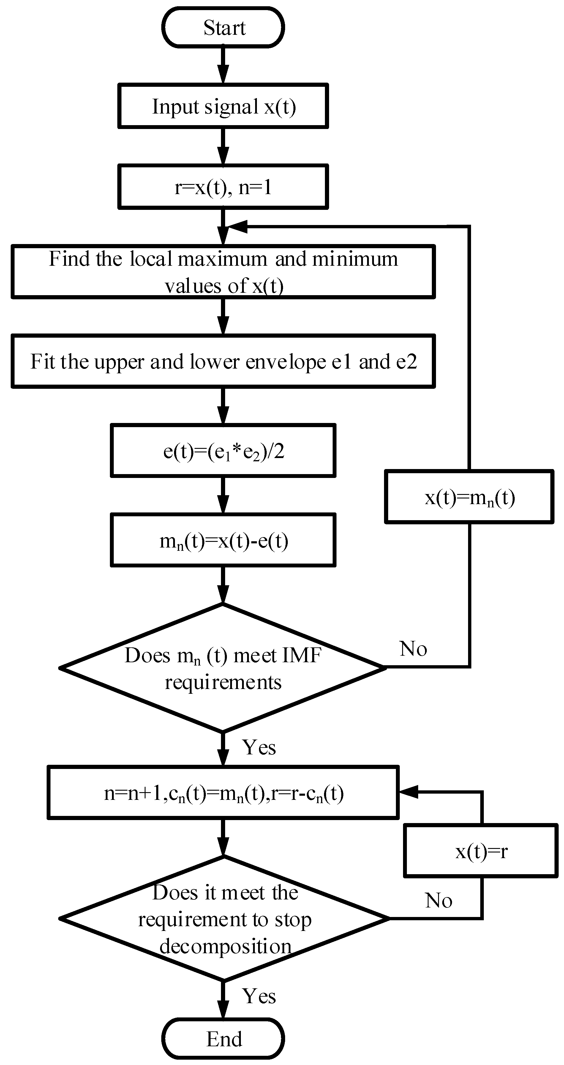
3.1. Signal Denoising Based on EMD

Hydropower units mainly include four types of faults: lifting accidents, excessive bearing temperature, insufficient power, and vibration faults. In case of a lifting accident, the pressure in the draft tube is insufficient, and a vacuum is formed in some areas, resulting in the water hammer phenomenon. This allows the unit to obtain a reverse axial force. When the force exceeds the gravity borne by the device, the rotating part of the device will move vertically upwards for a certain distance. When such accidents occur, the blades are prone to fracture under stress, damaging the unit cover, and even damaging important components such as the generator brush, causing serious and malignant accidents. In addition, cracks, cavitation, and erosion damage are important faults that require diagnosis. This study focuses on the vibration faults of hydropower units. Due to the fact that most vibration fault diagnosis signals of hydroelectric units do not have the characteristic conditions of IMFs, the instantaneous values of various signals cannot be obtained. By using EMD to solve for each order component, the signal can be decomposed into multiple IMFs, thereby achieving real-time noise reduction processing and feature extraction of the signal. Figure 1 shows the specific process of EMD processing.

All the maximum and minimum points in the original signal $x(t)$ are calculated, and the maximum envelope $e_{+}(t)$ and minimum envelope $e_{-}(t)$ are fitted. All the original signals are between two envelopes. According to Formula (1), the mean envelope D can be further solved.

$$e(t)=\frac{e_{+}(t)+e_{-}(t)}{2}$$

(1)

$$m_1(t)=x(t)-e(t)$$

(2)

According to Equation (2), the new signal $m_1(t)$ is obtained by subtracting $e(t)$ from the original signal $x(t)$. It is determined whether $m(t)$ meets the basic requirements of the IMF. If it does, $m_1(t)$ is the first-order IMF, represented by $c_1(t)$. If it does not meet the requirements, it is necessary to consider $m_1(t)$ as the original signal and continue solving until the $k$ solution meets the basic requirements of the IMF.

$$\{\begin{array}{c}{r}_1(t)=x(t)-c_1(t)\\ r_2(t)=x(t)-c_2(t)\\ ⋮\\ r_n(t)=x(t)-c_n(t)\end{array}$$

(3)

In Equation (3), it is necessary to further subtract $c_1(t)$ from the original signal $x(t)$ to obtain a new signal $r_1(t)$. By repeating the above operation, the eigenmode functions of the second, third, and $n$ orders can be obtained sequentially. The above process is the decomposition process of the empirical mode, which can ultimately decompose the original signal $x(t)$ into several IMF components and one participating function. The components of each IMF are used to represent the various frequency components in the original signal, while the residual function represents the overall average trend of the original signal. According to Equation (4), each function is summed.

$$x(t)={\displaystyle \sum _{i=1}^n{c}_i(t)+r_n(t)}$$

(4)

Noise reduction processing is the first step in diagnosing vibration fault signals, and using EMD can achieve noise reduction processing of different signals. In Figure 2, the energy of useful signals is generally smaller than that of noisy signals. When the signal-to-noise ratio is small, the overall energy of useful signals is relatively small, and it is easy for useful signals to be discarded during EMD. The high-frequency part of the useful signal is also easily discarded in decomposition, which may cause diagnostic bias of the fault signal and reduce the accuracy of diagnosis. For the vibration signal of hydroelectric units, noise usually appears in the high-frequency component and contains low energy. The high frequency is within 3~30 MHz. The effective signal is concentrated in the low-frequency part and contains high energy. The low frequency is within 30~300 KHz. Therefore, using empirical mode decomposition can conveniently remove high-frequency noise components from the collected vibration signals.

To solve the above problems, this study uses autocorrelation functions to reflect the similarity of the same signal at different times, to ensure that useful signals can be fully preserved in the case of a low signal-to-noise ratio. For the original signal $x(t)$ of infinite length, its autocorrelation function is defined by Equation (5).

$$R_x(t)={\displaystyle {\int }_{-\infty }^{+\infty }}x(t)x(t-\tau )dt$$

(5)

In Equation (5), $\tau$ is the delay time. The autocorrelation function value at zero point is the energy value of the original signal, represented by $R_x(0)$. The autocorrelation function is normalized according to Equation (6).

$${\rho }_x(t)=\frac{R_x(t)}{R_x(0)}$$

(6)

Since most of the vibration signals collected by hydropower units are discrete signals, Equations (5) and (6) need to be discretized before modal decomposition, and finally Equations (7) and (8) can be obtained.

$$R(n)={\displaystyle \sum _{k=-\infty }^{+\infty }x(k)x(k-n)dt}$$

(7)

$$\rho (n)=\frac{R(n)}{R(0)}$$

(8)

Based on the above content, it can be seen that a method is needed to determine the k value of the EMD function even when the signal-to-noise ratio is not high. Therefore, the concept of autocorrelation function was introduced in the experiment. The autocorrelation function reflects the similarity of a signal at two different times. Due to the weak correlation of noise signals at different times, their autocorrelation function decays rapidly, except for being larger at t = 0. For useful signals, there is a certain degree of correlation between different moments, and the autocorrelation function used does not have the characteristic of rapid decay. This characteristic can distinguish between noisy signals and useful signals. For the autocorrelation function of a finite-length original signal, the upper and lower limits of the accumulation in Equation (7) are the intersection of $x(t)$ and $x(t-n)$. The IMF of the high frequency is determined by the noise signal. Sometimes the intrinsic mode function of the high frequency is dominated by noise signals. However, there are some useful signals mixed among them, and sometimes the noise and useful components of a certain component both contain a significant proportion. At this point, this component cannot be directly discarded; otherwise, some useful information will be lost. Therefore, in the experiment, another common denoising method in the field of signal processing, namely wavelet threshold denoising, was borrowed to inspire the processing method of empirical modal threshold denoising. To preserve the useful mixed signals in these signals, a threshold denoising method is studied and introduced. The process involves obtaining a series of wavelet coefficients through wavelet processing. Subsequently, a threshold function is used to analyze and process the wavelet coefficients to achieve the purpose of noise reduction processing. The threshold function mainly includes a hard threshold function and a soft threshold function, and their formulas are shown in Equations (9) and (10), respectively.

$${\widehat{w}}_x=\{\begin{array}{l}{w}_x,\left|w_x\right|\ge \lambda \\ 0,\left|w_x\right|<\lambda \end{array}$$

(9)

$${\widehat{w}}_x=\{\begin{array}{l}\mathrm{sgn}(w_x)(\left|w_x\right|-\lambda ),\left|w_x\right|\ge \lambda \\ 0,\left|w_x\right|<\lambda \end{array}$$

(10)

In Equations (9) and (10), ${\widehat{w}}_x$ and $w_x$ are the wavelet coefficients before and after denoising, $\mathrm{sgn}(\ast )$ is the sign function, and $\lambda$ means the threshold.

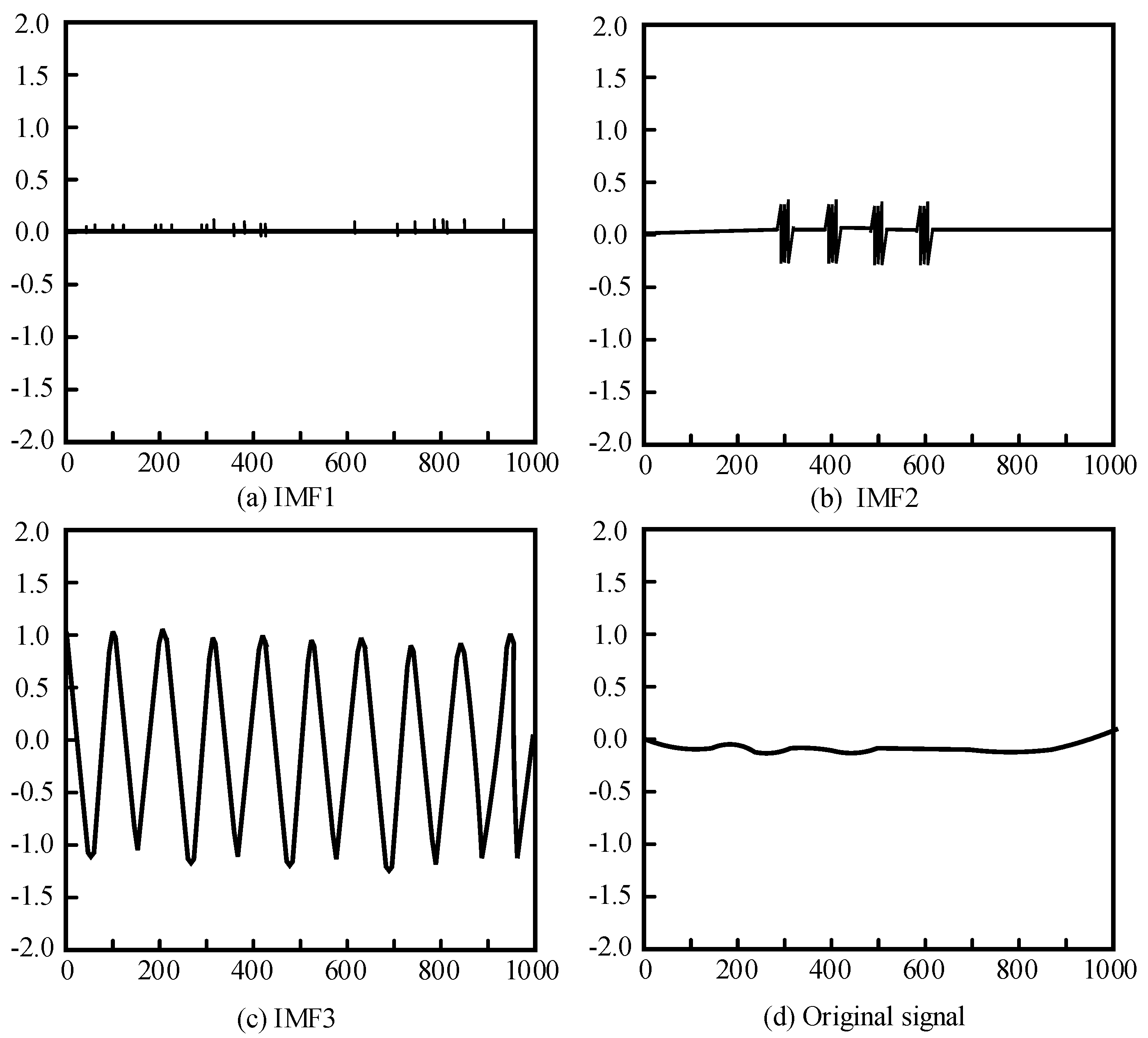
3.2. Vibration Signal Feature Extraction Based on EMD Theory

Signal feature extraction is the main step in fault diagnosis, and the use of EMD theory can also achieve the extraction of signal feature information. According to the empirical mode noise reduction theory in Section 3.1, the endpoints of the maximum and minimum envelopes are not necessarily the extreme points of the real signal. Therefore, the divergence problem, namely the endpoint effect, is prone to occur near the extreme endpoints. The methods for suppressing endpoint effects include polynomial fitting and mirror extension. Using the mirror extension method, one first needs to find the two closest extreme points to the left and right ends and then flip the curve between these two extreme points to fit the nearest extreme point outside the endpoint. The signal after splitting and extending was decomposed using empirical mode decomposition, and the obtained components of each order were intercepted from the parts between the original left and right endpoints. After processing, it can be ensured that the function value at the endpoint is indeed an extreme value. However, there are also some defects. For the original signal, there is a need to discard some data and replace it with data after mirror symmetry. In addition, the length of the signal may change, and after empirical mode decomposition, it is necessary to intercept some data of the components. The signal decomposition results obtained after using this processing method are shown in Figure 3. It can be seen that except for residual components with smaller amplitudes, the decomposition results are already very close to the ideal situation, which verifies the effectiveness of the method. This method requires less computation and has a more ideal effect. Therefore, this chapter chooses this method to reduce the impact of endpoint effects.

When two signals with significant time differences undergo modal decomposition, they may be divided into the same component, or signals with small time differences may be divided into different components. These phenomena are called modal aliasing. The main reason for mode aliasing is the problem of signal discontinuity. Aggregated EMD adds white noise to the original signal to obtain a new signal $x^{\ast }(t)$. The use of new signals for subsequent modal decomposition can compensate for missing parts in the time scale, thereby effectively reducing the phenomenon of modal aliasing. Figure 4 shows the results of aggregated EMD.

To reduce the negative impact of computer calculation on fault diagnosis and recognition, the characteristic parameters of the signal waveform are calculated for each order component. This can achieve feature extraction of signals to ensure the accuracy of fault signal recognition and diagnosis. After improving empirical mode decomposition, the vibration signal is divided into many order components. However, if these components are directly sent to the computer for fault diagnosis, excessive computation will also be interfered with by useless information, resulting in low diagnostic accuracy. Therefore, before fault diagnosis, it is necessary to calculate some characteristic parameters of the waveform. Compared with dimensional feature parameters, nondimensional feature parameters can avoid the impact of different dimensions on the overall goal. Therefore, this article selects nondimensional feature parameters as the basis for evaluation. This study uses 10 nondimensional feature parameters, namely coefficient of variation ($f_1$), skewness coefficient ($f_2$), peak skewness coefficient ($f_3$), valley skewness coefficient ($f_4$), kurtosis coefficient ($f_5$), peak kurtosis coefficient ($f_6$), valley kurtosis coefficient ($f_7$), peak-to-average ratio ($f_8$), margin coefficient ($f_9$), and energy ratio ($f_{10}$). To evaluate the fault sensitivity characteristic parameters, the detection index is introduced, and Equation (11) is its calculation formula.

$$f=\frac{\left|{\mu }_1-{\mu }_2\right|}{\sqrt{{\sigma }_1^2+{\sigma }_2^2}}$$

(11)

In Equation (11), it is assumed that $s_1$ and $s_2$ are the two characteristic parameters of the same state. ${\mu }_1$ and ${\mu }_2$ are the mean values of $s_1$ and $s_2$, respectively. ${\sigma }_1$ and ${\sigma }_2$ represent the variances of $s_1$ and $s_2$, respectively. When the detection index value is larger, the sensitivity of the feature parameters to different states is higher. To further demonstrate the recognition rate of fault signal feature extraction, the study uses the comprehensive detection index $S$ to represent the sum of all detection indices of the same characteristic parameter $s$, and Equation (12) is its calculation expression.

$$S={\displaystyle \sum f}$$

(12)

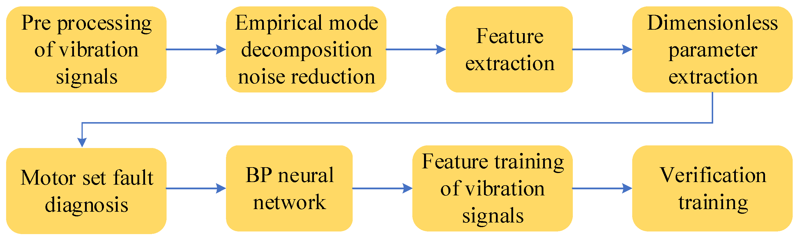
3.3. Application of BPNN in Vibration Fault Signals

The BPNN is a universal multilayer feedforward neural network. BP mainly obtains new knowledge by imitating feature extraction and training in the cognitive process, and it adjusts the network weights and thresholds through backpropagation [29]. Due to its excellent performance in the collection, reception, and processing of information, it has the advantages of simple operation and high prediction accuracy. Therefore, the study adopts BPNN to establish a corresponding nonlinear relationship between the vibration fault signal characteristics and the operating status of hydroelectric units, which can achieve intelligent diagnosis and recognition of hydroelectric unit faults. As shown in Figure 5, the traditional BPNN algorithm structure consists of three hierarchical structures. The operation process mainly includes two processes: forward information transmission and backward error transmission.

Forward transmission is the process in which the input value interacts with the weight threshold through the hidden layer and is finally output by the output layer. The neuron number is represented by $n$ in the input layer and $m$ in the output layer. Their serial numbers are represented by $i$ and $j$. The specific operation process is shown as follows:

$$y_i=f({\displaystyle \sum _{i=1}^n{w}_{ij}{x}_i-{\theta }_j})$$

(13)

$$z_k=f({\displaystyle \sum _{j=1}^l{w}_{jk}{y}_j-{\theta }_k})$$

(14)

In Equations (13) and (14), $x$ is the vector of the input layer, $y$ is the vector of the hidden layer, and $z$ represents the vectors of the output layer. $\theta$ is the neuron threshold of the hidden layer, and $w$ represents the weight of the hidden layer. Reverse transmission compares the output results with the preset conditions. The output values that do not meet the requirements are returned to the neural network for the next transmission until the preset conditions are met. The expected output vector is represented by $z^{\ast }$, and the error between the output result and the expected value is represented by $E$. Equation (15) is the calculation of the error.

$$E=\frac{1}{2}{\displaystyle \sum _{k=1}^m{(z_k^{\ast }-z_k)}^2}$$

(15)

Error backpropagation is the process of adjusting the weight threshold of the hidden layer based on the error. The specific operation process is shown in Equations (16)–(19), where $\eta$ is the step size of weight threshold adjustment. In the experiment, the weights and thresholds are adjusted based on the negative error gradient. After the reverse transmission is completed, the information can be transmitted forward again until the preset termination conditions are met.

$$\Delta w_{jk}=-\eta \frac{\partial E}{\partial w_{jk}}=\eta (z_k^{\ast }-z_k)y_i{f}^{\prime }({\displaystyle \sum _{j=1}^l{w}_{jk}{y}_j-{\theta }_k})$$

(16)

$$\Delta {\theta }_k=-\eta \frac{\partial E}{\partial {\theta }_k}=\eta (z_k-z_k^{\ast })f^{\prime }({\displaystyle \sum _{j=1}^l{w}_{jk}{y}_j-{\theta }_k})$$

(17)

$$\Delta w_{jk}=-\eta \frac{\partial E}{\partial w_{jk}}=\eta x_i{f}^{\prime }({\displaystyle \sum _{i=1}^n{w}_{ij}{x}_i-{\theta }_j}){\displaystyle \sum _{j=1}^l{w}_{jk}{f}^{\prime }({\displaystyle \sum _{j=1}^l{w}_{jk}{y}_j-{\theta }_k})}(z_k^{\ast }-z_k)$$

(18)

$$\Delta {\theta }_j=-\eta \frac{\partial E}{\partial {\theta }_j}=\eta f^{\prime }({\displaystyle \sum _{i=1}^n{w}_{ij}{x}_i-{\theta }_j}){\displaystyle \sum _{k=1}^m{w}_{jk}{f}^{\prime }({\displaystyle \sum _{j=1}^l{w}_{jk}{y}_j-{\theta }_k})}(z_k-z_k^{\ast })$$

(19)

The dimensionless feature parameters used for fault evaluation are scaled proportionally to serve as input vectors for the neural network, which can determine the number of neurons in the output layer. The output layer represents the specific operating state, with a neuron number of 1. For the activation function of the hidden layer, the double S-type activation function with high convergence accuracy and efficiency is selected. The hidden layer is different from the visible layer, and its number of neurons needs to be specified by the user according to the situation. Too few or too many neurons may cause nonconvergence or lower recognition ability. However, nowadays, the selection of the number of neurons in the hidden layer lacks a theoretical basis, and empirical formulas are usually used. The value of α is finally determined through multiple experiments. The hidden layer neuron number is calculated using the empirical Formula (20), and $\alpha$ values are in [1,14].

$$m=\sqrt{n+1}+\alpha$$

(20)

It has been found that the average accuracy of fault diagnosis using conjugate gradient algorithms is relatively high. Therefore, the conjugate gradient algorithm was chosen as the training algorithm for the neural network in the study. In the experiment, the number of input layer nodes for BPNN was set to 6, the number of output layer nodes was set to 4, and the number of hidden layer nodes was set to 11. The number of training samples was 50, each sample contained 1024 sampling points, and the training time was 0.0762 s. The learning rate was 0.001.

A flowchart of the whole model is presented in Figure 6. The first step was to preprocess the vibration signal. The experimental mode decomposition was introduced for noise reduction in the experiment. Then there is the feature extraction of vibration signals. Different dimensionless parameters were compared and extracted. Finally, the fault diagnosis of hydroelectric units was based on BP neural network. It was necessary to train the features of the extracted vibration signal. Then, validation training was conducted to determine the accuracy of fault diagnosis.

4. Simulation of Vibration Signal Fault Diagnosis Experiment for Three Hydroelectric Units

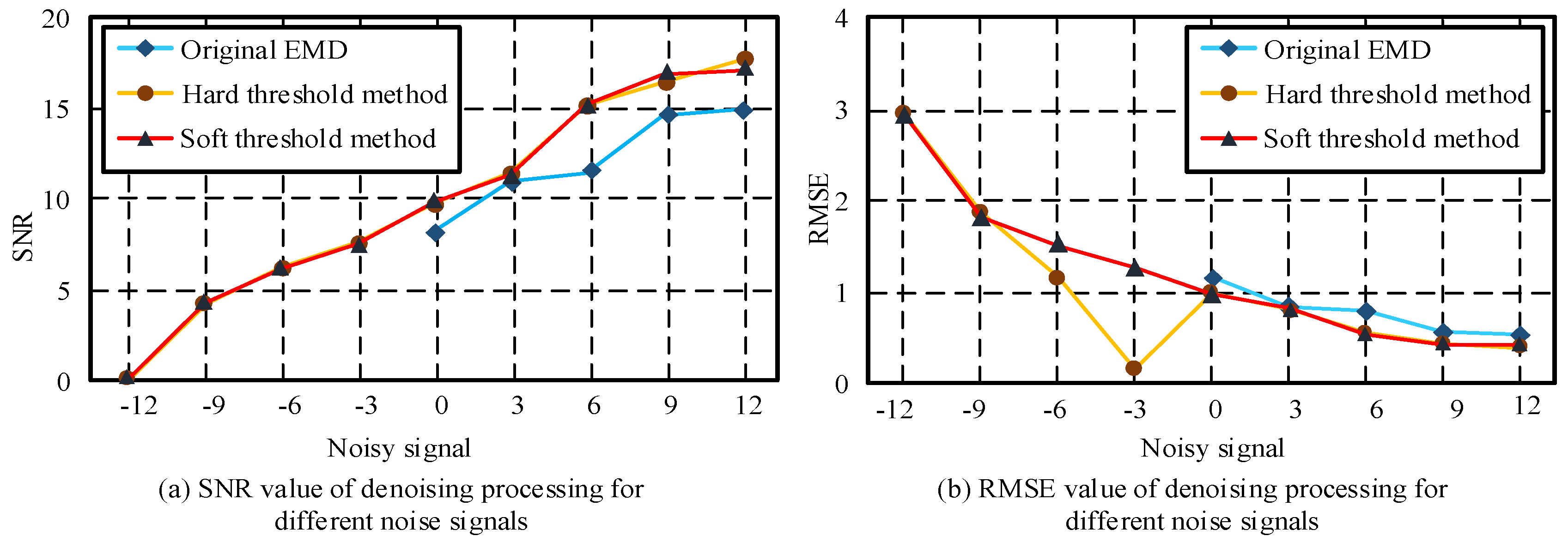
4.1. Vibration Signal Denoising Processing

The model of the water turbine generator was a 50 MW ZZ-LH-5953 axial flow propeller-type water turbine generator. The testing system was a noncontact vibration testing system containing a laser Doppler vibrometer (LDV). The diameter of the fault point was 0.178 mm. The study first conducted experimental simulation analysis on the application of improved EMD in the denoising process of vibration signals of hydroelectric units. The evaluation criteria for the effectiveness of noise reduction processing were signal-to-noise ratio (SNR) and root mean square (RMSE). The evaluation standard used in the experiment was ISO 20816. The block signal was a standard test signal generated by MATLAB. The experiment mainly used the blocks as a signal without noise, with 1024 signal sampling points. A white noise signal was randomly added on the basis of pure signal, and the signal-to-noise ratio of the noise signal was $\left[-12,-9,-6,\cdots 6,9,12\right]\mathrm{dB}$. EMD was performed on each noisy signal to obtain nine-order components. According to the autocorrelation function results, the first three orders were the dominant IMFs and could be omitted. The remaining sixth-order components were superimposed and reconstructed again to obtain a denoised signal. Figure 7 shows the comparison results of different denoising methods.

In the case of a low signal-to-noise ratio, the original EMD cannot achieve noise reduction processing. In the case of a high signal-to-noise ratio, all three methods can be used for noise reduction. However, compared to the original EMD, the improved method has higher noise reduction performance. The original EMD and the improved method were used to denoise the vibration signals of the hydroelectric unit under normal operation, misalignment, imbalance, and friction conditions. Misalignment is one of the most common faults in hydraulic machinery [30]. The rotor system of hydropower units with misalignment faults operates relatively unstably, and obvious first harmonic vibration can be observed on the upper and lower frames of the hydropower units. The oscillation amplitude of the hydroelectric unit monitored near the generator guide bearing and the hydraulic turbine guide bearing will also significantly increase, leading to a decrease in the efficiency of the hydroelectric unit. There are many reasons for misalignment faults in the rotor system of hydroelectric units. The most common is that insufficient manufacturing accuracy leads to rotor bending, or low installation accuracy leads to rotor misalignment, bending, etc. The imbalance state of hydroelectric units is a random combination of static imbalance and torque imbalance, and the mass centerline of the shaft is neither parallel to nor intersecting with the rotation centerline. This can cause the vibration of water turbine generator sets and reduce the service life of instruments. The friction state refers to friction between the rotating and fixed components of a hydroelectric unit. The noise signals vary in different situations, and detailed distinctions were made in the experiment for these four situations. Figure 8 shows the signals obtained under the first four operating states of noise reduction processing.

An improved method was used to denoise the vibration signals of hydroelectric units in normal operation, misalignment, imbalance, and friction conditions. The frequency was set at 1024 Hz, and the shaft speed was set at 1200 rpm. Fifty sets of signals were collected for each operating state, each containing 2048 sampling points. Figure 9 shows the signals obtained under four operating states after noise reduction processing.

By analyzing Figure 8 and Figure 9, compared with the original signal, it can be seen that the denoised signal has significantly reduced burrs and the trend of change is easier to analyze and judge. In the experiment, the signal capability of noise in each state before and after noise reduction was calculated separately. The comparison results showed that after denoising, the signal energy in normal operation, misalignment, balance, and friction conditions decreased by 3%, 7%, 12%, and 15%, respectively. This indicates that the improved EMD in this study can effectively achieve signal denoising, laying a foundation for subsequent fault diagnosis.

4.2. Fault Signal Feature Extraction and Diagnosis

The denoised signal was further subjected to EMD, and 10 characteristic parameters of each order component were calculated. Each group of signals was decomposed into five orders, resulting in a total of 50 characteristic parameter values. According to the calculation formula in Section 3.2, the comprehensive detection index of the feature parameters in Figure 10 can be calculated.

The peak skewness coefficient ($f_3$), valley skewness coefficient ($f_4$), and kurtosis coefficient ($f_5$) have the highest mean detection index values. The detection index values of the second- and third-order components of the three parameters have a larger mean. For this study, it was determined to use the $f_3$, $f_4$, and $f_5$ parameters of the second- and third-order components as the evaluation criteria for subsequent fault signal diagnosis. This study contains a total of six feature parameters, which determines the number of neurons in the BPNN input layer to be six. Here, 0, 1, 2, and 3 are used to represent the normal state, misalignment state, imbalance state, and collision state of the hydroelectric unit operation. The identification and diagnosis results of different states are shown in Figure 11 (partially displayed).

The average recognition rate for each different state was calculated to be 90.6%. In the experiment, the accuracy of diagnosis is judged based on whether there is a difference between the actual state and the detected vibration signal. The “average accuracy of fault diagnosis” is the average value after multiple measurements. The average accuracy of recognition diagnosis is 96.2%. It indicates that using BPNN combined with EMD can achieve intelligent identification of vibration fault signals in hydroelectric units.

4.3. Comparison of Signal Fault Diagnosis Methods

For the comparison of signal fault diagnosis methods for hydropower units, the MIMII public dataset [31] was used. In the comparative experiment, the sounds of fans, valves, water pumps, and sliding rails during operation were collected. Precision, recall, and their ratio F1 value, as well as the area under the subject’s working curve, were selected as performance testing indicators for the abnormal sound detection method in the study. In

Table 1. Comparison results of indicators for different methods.

Method	Fan				Water Pump
	Precision	Recall	F1	AUC	Precision	Recall	F1	AUC
Adaptive filtering algorithm [32]	0.9049	0.5672	0.6753	0.6712	0.7447	0.6773	0.6886	0.7437
BP neural network [33]	0.8926	0.1724	0.2672	0.6315	0.7722	0.2060	0.3142	0.6865
EMD + SVM [34]	0.8528	0.2152	0.3264	0.6019	0.7529	0.3662	0.4733	0.6875
This paper	0.9405	0.4172	0.5356	0.7365	0.7375	0.5162	0.5753	0.7335
Method	Slide Rail				Valve
	Precision	Recall	F1	AUC	Precision	Recall	F1	AUC
Adaptive filtering algorithm [32]	0.8487	0.7743	0.8069	0.8651	0.6671	0.2836	0.3968	0.6763
BP neural network [33]	0.6202	0.0490	0.0888	0.6376	0.3132	0.0388	0.0684	0.4825
EMD + SVM [34]	0.7365	0.1979	0.3101	0.5845	0.6151	0.1786	0.2764	0.5152
This paper	0.8947	0.9007	0.8957	0.9232	0.8763	0.6712	0.7355	0.9141

, these indicators are used to compare the performance of the methods in this study with those in the literature.

From the results in Table 1, it can be seen that this paper’s method has a high AUC value, with AUC values of 0.7365, 0.7335, 0.9232, and 0.9141 for fan, water pump, slide rail, and valve sound detection, respectively, with an average AUC value of 0.8268. This paper’s method increased the AUC value by 11.8722% compared to the method in [32], 35.6518% compared to the method in [33], and 38.4322% compared to the method in [34].

The accuracy and loss function of different methods are compared in Figure 12. In the accuracy comparison chart, the accuracy of the proposed model in this experiment is 90.1%. The accuracy in [28] is 87.2%. The accuracy in [29] is 81.7%. The accuracy in [30] is 80.0%. In the comparison diagram of the loss function, the loss function value of this paper’s method is 0.19. The loss function value in [28] is 0.27. The loss function value in [29] is 0.30. The loss function value in [30] is 0.42. From the comparison of the accuracy and loss function, it can be seen that this paper’s intelligent fault analysis model has a faster convergence speed and higher accuracy.

5. Conclusions

Extracting information based on the vibration signal characteristics of hydroelectric units can identify the operating status of hydroelectric units, thereby achieving intelligent diagnosis and recognition of hydroelectric unit faults. In response to the problem of low recognition accuracy in fault diagnosis of hydropower units at present, this study adopts an improved empirical modal component theory and the BPNN to study and analyze the denoising, feature extraction, and fault signal recognition process of hydropower unit signals. The simulation results show that the improved empirical modal components obtained in this study have the advantages of wide noise reduction surface and good noise reduction performance and can handle noise signals with different levels of interference. At the same time, the fault signal of hydroelectric units can be distinguished by three dimensionless feature parameters: peak skewness coefficient, valley skewness coefficient, and kurtosis coefficient of the second-order and third-order components of the signal. The BPNN simulation results show that the recognition rate for faults in hydroelectric units can reach 90.6%, and the recognition accuracy can reach 96.2%. The method proposed in this experiment has a high AUC value, with AUC values of 0.7365, 0.7335, 0.9232, and 0.9141 for fan, water pump, slide rail, and valve sound detection, respectively, with an average AUC value of 0.8268. This paper’s method increased the AUC value by 11.8722% compared to the method in [18], 35.6518% compared to the method in [19], and 38.4322% compared to the method in [20]. At the same time, the accuracy rate of the model proposed in this experiment is 90.1%, and the loss function value is 0.27, both higher than those of the methods in the literature. Although this study has achieved intelligent recognition of vibration fault signals in hydroelectric units and improved the recognition rate and accuracy of fault signals, simplifying the fault signal recognition process and expanding the scope of fault monitoring are the main directions that require continuous efforts in research.

References

1. Fan, Q.X.; Deng, Z.Y.; Lin, P.; Li, G.; Fu, J.L.; He, W. Coordinated deformation control technologies for the high sidewall—Bottom transfixion zone of large underground hydro-powerhouses. J. Zhejiang Univ. Sci. A 2022, 23, 543–563. [Google Scholar] [CrossRef]
2. Pandey, M.; Winkler, D.; Vereide, K.; Sharma, R.; Lie, B. Mechanistic model of an air cushion surge tank for hydro power plants. Energies 2022, 15, 2824. [Google Scholar] [CrossRef]
3. Ilak, P.; Kuzle, I.; Lin, H.; Akovic, J.; Rajsl, A.I. Market power of coordinated hydro-wind joint bidding: Croatian power system case study. J. Mod. Power Syst. Clean Energy 2022, 10, 531–541. [Google Scholar] [CrossRef]
4. Xu, Y.C.; Xia, H.T.; Fang, S.C.; Lu, M. Research on APSO-WNN and its Application in Vibration Fault Diagnosis of Hydroelectric Generating Units. J. Chin. Soc. Mech. Eng. Ser. C Trans. Chin. Soc. Mech. Eng. 2021, 42, 163–172. [Google Scholar]
5. Dao, F.; Zeng, Y.; Zou, Y.; Li, X.; Qian, J. Acoustic vibration approach for detecting faults in hydroelectric units: A review. Energies 2021, 14, 7840. [Google Scholar] [CrossRef]
6. Rong, J.; Ge, H. April. Hydroelectric generating unit vibration fault diagnosis via BP neural network based on particle swarm optimization. In Proceedings of the 2009 International Conference on Sustainable Power Generation and Supply, Nanjing, China, 6–7 April 2009; pp. 1–4. [Google Scholar]
7. Min, H.G.; Fang, Y.K.; Wu, X.; Lei, X.P.; Chen, S.X.; Teixeira, R.; Zhu, B.; Zhao, X.M.; Xu, Z.G. A fault diagnosis framework for autonomous vehicles with sensor Self-Diagnosis. Expert Syst. Appl. 2023, 224, 120002. [Google Scholar] [CrossRef]
8. Xu, S.Q.; Huang, W.Z.; Huang, D.R.; Chen, H.T.; Chai, Y.; Ma, M.Y.; Zheng, W.X. A reduced-order observer-based method for simultaneous diagnosis of open-switch and current sensor faults of a grid-tied NPC inverter. IEEE Trans. Power Electron. 2023, 38, 9019–9032. [Google Scholar] [CrossRef]
9. Chen, H.; Xiong, Y.; Li, S.; Song, Z.; Hu, Z.; Liu, F. Multi-sensor data driven with PARAFAC-IPSO-PNN for identification of mechanical nonstationary multi-fault mode. Machines 2022, 10, 155. [Google Scholar] [CrossRef]
10. Cheng, C.; Wang, J.; Zhou, Z.; Teng, W.; Sun, Z.; Zhang, B. A BRB-based effective fault diagnosis model for high-speed trains running gear systems. IEEE Trans. Intell. Transp. Syst. 2022, 23, 110–121. [Google Scholar] [CrossRef]
11. Chen, H.X.; Liu, M.M.; Chen, Y.T.; Li, S.Y.; Miao, Y.Z. Nonlinear lamb wave for structural incipient defect detection with sequential probabilistic ratio test. Secur. Commun. Netw. 2022, 2022, 9851533. [Google Scholar] [CrossRef]
12. Xiong, J.; Li, C.; Wang, C.D.; Cen, J.; Wang, Q.; Wang, S. Application of convolutional neural network and data preprocessing by mutual dimensionless and similar gram matrix in fault diagnosis. IEEE Trans. Ind. Inform. 2022, 18, 1061–1071. [Google Scholar] [CrossRef]
13. Hichri, A.; Hajji, M.; Mansouri, M.; Abodayeh, K.; Bouzrara, K.; Nounou, H. Genetic-algorithm-based neural network for fault detection and diagnosis: Application to grid-connected photovoltaic systems. Sustainability 2022, 14, 10518. [Google Scholar] [CrossRef]
14. Khr, A.; Smm, B.; Ma, B. Lung cancer diagnosis based on chan-vese active contour and polynomial neural network. Procedia Comput. Sci. 2021, 194, 22–31. [Google Scholar]
15. Li, H.T.; Yuan, S. Corrosion prediction of marine engineering materials based on genetic algorithm and BP neural network. Mar. Sci. 2021, 44, 33–38. [Google Scholar]
16. Yan, J.; Pan, Z.; Tan, J.; Tian, H. Assessment of water quality by firefly algorithm based on BP neural network model. SouthtoNorth Water Transf. Water Sci. Technol. 2020, 1, 104–110. [Google Scholar]
17. Chi, C.; Pan, Z.; Zhao, X.; Zhang, Y. Power converter fault classification method based on multi-feature selection algorithm. J. Northwestern Polytech. Univ. 2022, 40, 645–650. [Google Scholar] [CrossRef]
18. Shi, Y.; Zhou, J.; Huang, J.; Xu, Y.; Liu, B. A Vibration Fault Identification Framework for Shafting Systems of Hydropower Units: Nonlinear Modeling, Signal Processing, and Holographic Identification. Sensors 2022, 22, 4266. [Google Scholar] [CrossRef]
19. Zhang, J.; Cheng, Z. Prediction of Surface Subsidence of Deep Foundation Pit Based on Wavelet Analysis. Processes 2023, 11, 107. [Google Scholar] [CrossRef]
20. Trybek, P.; Sobotnicka, E.; Wawrzkiewicz-Jałowiecka, A.; Machura, Ł.; Feige, D.; Sobotnicki, A.; Richter-Laskowska, M. A New method of identifying characteristic points in the impedance cardiography signal based on empirical mode decomposition. Sensors 2023, 23, 675. [Google Scholar] [CrossRef]
21. Xu, F.H.; Wang, Z.; Liu, J.; Ning, Q.; Yu, Y. Acoustic logging information extraction and fractural volcanic formation characteristics based on empirical mode decomposition. Geophys. Prospect. Pet. 2022, 57, 936–943. [Google Scholar]
22. Pei, S.; Yin, X.; Li, K. Full-time domain matching pursuit and empirical mode decomposition based sparse fixed-point seismic inversion. J. Geophys. Eng. 2022, 19, 255–268. [Google Scholar] [CrossRef]
23. Ho, R.; Hung, K. EEG analysis and classification based on cardinal spline empirical mode decomposition and synchrony features. Med. Biol. Eng. Comput. J. Int. Fed. Med. Biol. Eng. 2022, 60, 2359–2372. [Google Scholar] [CrossRef] [PubMed]
24. Li, Z.; Jiang, W.; Zhang, S.; Sun, Y.; Zhang, S. A hydraulic pump fault diagnosis method based on the modified ensemble empirical mode decomposition and wavelet kernel extreme learning machine methods. Sensors 2021, 21, 2599. [Google Scholar] [CrossRef]
25. Toma, R.N.; Kim, C.H.; Kim, J.M. Bearing fault classification using ensemble empirical mode decomposition and convolutional neural network. Electronics 2021, 10, 1248. [Google Scholar] [CrossRef]
26. Liu, Z.; Zhou, J.; Zou, M.; Zhang, Y.; Zhan, L. A new method for intelligent fault diagnosis of hydroelectric generating unit. In Proceedings of the 2007 IEEE International Conference on Control and Automation, Guangzhou, China, 17–20 October 2007; pp. 1638–1642. [Google Scholar]
27. Jana, D.; Nagarajaiah, S.; Yang, Y.; Li, S. Real-time cable tension estimation from acceleration measurements using wireless sensors with packet data losses: Analytics with compressive sensing and sparse component analysis. J. Civ. Struct. Health Monit. 2021, 12, 797–815. [Google Scholar] [CrossRef]
28. Jana, D.; Patil, J.; Herkal, S.; Nagarajaiah, S.; Duenas-Osorio, L. CNN and Convolutional Autoencoder (CAE) based real-time sensor fault detection, localization, and correction. Mech. Syst. Signal Process. 2022, 169, 108723. [Google Scholar] [CrossRef]
29. Liao, H.C.; Liao, H.C.; Gao, Y.; Gao, Y.; Wang, Q.G.; Dan, W. Development of viscosity model for aluminum alloys using BP neural network. Trans. Nonferrous Met. Soc. China 2021, 31, 2978–2985. [Google Scholar] [CrossRef]
30. Kumar, P.; Tiwari, R. A review: Multiplicative faults and model-based condition monitoring strategies for fault diagnosis in rotary machines. J. Braz. Soc. Mech. Sci. Eng. 2023, 45, 282. [Google Scholar] [CrossRef]
31. Zabin, M.; Choi, H.J.; Uddin, J. Hybrid deep transfer learning architecture for industrial fault diagnosis using Hilbert transform and DCNN–LSTM. J. Supercomput. 2023, 79, 5181–5200. [Google Scholar] [CrossRef]
32. Wu, Y.; Zhang, Z.; Li, Y.; Sun, Q. Open-circuit fault diagnosis of six-phase permanent magnet synchronous motor drive system based on empirical mode decomposition energy entropy. IEEE Access 2021, 9, 91137–91147. [Google Scholar] [CrossRef]
33. Wei, M.; Hu, X.; Yuan, H. Residual displacement estimation of the bilinear SDOF systems under the near-fault ground motions using the BP neural network. Adv. Struct. Eng. 2022, 25, 552–571. [Google Scholar] [CrossRef]
34. Abou-Abbas, L.; Noordt, S.V.; Desjardins, J.A.; Cichonski, M.; Elsabbagh, M. Use of empirical mode decomposition in erp analysis to classify familial risk and diagnostic outcomes for autism spectrum disorder. Brain Sci. 2021, 11, 409. [Google Scholar] [CrossRef] [PubMed]
Figure 1. EMD process.
Processes 11 02040 g001
Figure 2. Schematic diagram of the comparison between useful signals and noise signals.
Processes 11 02040 g002
Figure 3. Schematic diagram of mirror extension.
Processes 11 02040 g003
Figure 4. Schematic diagram of aggregated EMD.
Processes 11 02040 g004
Figure 5. BPNN.
Processes 11 02040 g005
Figure 6. Flowchart of the whole model.
Processes 11 02040 g006
Figure 7. SNR and RMSE values after denoising using different methods.
Processes 11 02040 g007
Figure 8. Vibration signals of hydroelectric units in different operating states before noise reduction treatment.
Processes 11 02040 g008
Figure 9. Vibration signals of hydroelectric units under different operating states after noise reduction treatment.
Processes 11 02040 g009
Figure 10. Comprehensive detection index of feature parameters.
Processes 11 02040 g010
Figure 11. Neural network discriminant result graph.
Processes 11 02040 g011
Figure 12. Accuracy and loss function variation of different methods [28,29,30].
Processes 11 02040 g012