Research on Coupling Adsorption Experiments for Wall–Climbing Robots in Coal Mine Shafts

Abstract

Based on the composite shaft lining structure, the research on the electromagnetic and negative pressure coupling adsorption technology of wall–climbing robots is of great significance to improve the level of safety monitoring during the construction and service of coal mine shafts. On the basis of theoretical research and computational data, the numerical simulation and simulation experiments of the coupled adsorption system of a wall–climbing robot are conducted in this research. In the ANSA software environment, of experimental models and experimental environments of electromagnetic and negative pressure adsorption devices are constructed to investigate, parameters such as air flow and the law behavior of fan pressure under different system conditions, including negative pressure and varying fan speeds. The intensity distribution of the magnetic flux inside the electromagnetic circuit under different working conditions and the law of change in the direction of movement are explored. Furthermore, the power consumption and power increment of the electromagnetic and negative pressure adsorption system under the same adsorption force output are compared and analyzed. Based on the experimental results, a series of conclusions are verified; firstly the negative pressure of the system should be formed under certain basic specific fundamental conditions; secondly, the main velocity of the negative pressure adsorption system and the full pressure of the fan are determined by the internal and external pressure difference and the fan speed, respectively; lastly, the adsorption efficiency of electromagnetic adsorption is significantly higher than that of negative pressure adsorption. These research findings are expected to introduce a new technical means approach for the safety monitoring of vertical shafts and shafts in coal mines, thereby demonstrating the theoretical significance and practical value of the application and development of an underground multi–scenario robot automation system in coal mines.

1. Introduction

As the primary channel for transporting finished coal products, personnel, equipment, and other important materials, the safety of coal mine shafts is related to the safe production of the entire coal mine, which is deemed as the top–priority component of the coal mine safety system [1,2]. In the past few years, intelligent mining inspection robots, which integrate coal mine safety monitoring and robotics, have been widely applied in the field of the underground safety inspection of coal mines [3,4]. Using the wall climbing method, the intelligent monitoring robot completes the work tasks; therefore, the working space of the robot is expanded. Moreover, due to the limited working space in vertical shafts, it is difficult to conduct safety monitoring, and this technical issue is overcome [5,6] accordingly. During the construction phase of the shaft, and under the premise that the production equipment, power supply cables, and communication methods are uncertain and unstable, resource consumption is minimized, while the monitoring function is maximized. During the service period of the well shaft, by replacing manual daily safety inspections, the effectiveness and timeliness of monitoring data are improved, and the purpose of saving costs without affecting the normal production of coal mines is achieved, which is of great value for its practical application.

The key technologies of wall–climbing robots revolve around their adsorption capacity and motor capabilities. In view of how to solve the hindering effect of one’s own gravity during wall climbing, a variety of methods are tried by researchers at home and abroad, namely, negative pressure adsorption [7,8], bionics adsorption [9,10], climbing adsorption [11,12] and electromagnetic adsorption technology [13,14]. Those technologies have their own merits and demerits; consequently, it is essential to select according to the actual situation and specific needs. Combined with the structural characteristics of the composite well shaft lining and the gas properties in the working environment, the analysis indicates that the permanent magnet adsorption uses high–power magnets to form a stable magnetic field. There is no need for a power supply and control system, merely the structural design and mechanical properties of the robot body should be taken into account, and there is no danger of slipping even when the system is suddenly powered down [15,16].

However, the biggest defect of permanent magnet adsorption is that it is impossible to adjust the adsorption force dynamically. The adsorption force generated at any moment remains unchanged. To ensure reliable adsorption, the adsorption force generated must be greater than the maximum adsorption force required at all times during the robot’s crawling process. Excessive adsorption force increases the pressure and friction of the drive wheel on the wall. The drive system has to deliver more energy to ensure the normal movement of the robot, causing excessive energy consumption and affecting the flexibility of movement. Due to the use of the magnetic force of the magnetic field generated by the electromagnetic equipment on the ferromagnetic material as the adsorption source, the electromagnetic adsorption is not affected by the smoothness of the lining, bringing it better lining surface adaptability. The electromagnetic adsorption force can be adjusted by voltage [17,18]; however, due to the limitations of the shaft lining structure, it is difficult to achieve a fully reliable adsorption guarantee in areas where the reinforcement bar spacing is too wide or the concrete protective layer is too thick. Based on the principles of fluid mechanics and pneumatic aerothermodynamics, a negative pressure mechanism is used to create the pressure difference between the air in the cavity and the external atmosphere; thus, the negative pressure adsorption force is generated. Getting rid of the limitations of lining structure and material, the mechanism of the negative pressure–generating system of the negative pressure adsorption method is relatively simple, which can provide a stable adsorption guarantee [19,20]. Meanwhile, in areas where the shaft lining is too rough or in ravines or protrusions, the inevitable hazard of losing negative pressure due to excessive air leakage from the sealing mechanism may occur occasionally.

The previous research on the application of wall–climbing robots in the industrial field was normally limited to merely a single scenario. It was either electromagnetic adsorption on a planar guide magnet or negative pressure adsorption on a smooth surface, which made it more demanding on the adsorption conditions of the vertical lining. The lack of in–depth research on complex environmental applications or coupled adsorption technologies made it difficult for wall–climbing robots to be widely used in industrial production and civil life. In the practical application of wall–climbing robot technology in the safety monitoring of coal mine shafts, due to the composite shaft lining structure and rough surface commonly used in the coal mine shaft’s lining, it was difficult to provide safe and stable adsorption pressure for the wall–climbing robot with a single adsorption method. As a result, based on the structural characteristics of reinforced concrete on the inner lining of the well shaft, the electromagnetic adsorption device and the negative pressure adsorption device that meet the actual needs are designed to produce electromagnetic adsorption and negative pressure adsorption to achieve complementary effects, which are consistent with the lining adsorption requirements of wall–climbing robots under the well shaft environment.

Taking the maximum negative pressure required by the system under independent negative pressure adsorption as the actual working condition point, through this research, the basic data and boundary values of the experimental entry conditions are set, the structural parameters and outlet and inlet angles of the centrifugal fan are calculated, and the pressure distribution, fluid flow, velocity component, and direction of movement at different stages of fluid movement are analyzed. The changes in the electromagnetic parameters of the electromagnetic channel of the electromagnetic unit and the reinforcement bar in the lining under changes in reinforcement bar model, posture angle, and coil current are explored. According to the experimental results, the formation mechanism of electromagnetic adsorption and negative pressure adsorption have been verified. Numerical analysis has revealed the feasibility and advanced nature of coupled adsorption technology. Moreover, based on the comparative analysis results of power loss under the same operating conditions, the law of change of system power with output adsorption force in the coupled adsorption mechanism and the general principle of electromagnetic and negative pressure adsorption power distribution in system’s operation are derived. In the simulation experiment of this paper, multiple inspection surfaces were established, and the investigation and analysis of the overall experimental process was highlighted, thereby avoiding the excessive singularity and one–sided situation in previous experimental research. Through the comparative analysis of the calculation results and the experimental results, the persuasiveness of the experimental conclusions was enhanced. Adopting the coupled adsorption method, the intelligent safety monitoring wall–climbing robot system can not only be applied for safety monitoring during the construction and production of coal mine shafts, but it can also be widely used in other non–ferrous metal mines, as well as in the local safety monitoring of civil engineering facilities such as railways and subway tunnels.

2. Admission Conditions for Negative Pressure Adsorption Experiment

(1)

Basic data of negative pressure adsorption experiment

For the digital simulation experiment of the negative pressure adsorption mechanism of the wall–climbing robot, in the preparation stage of the experiment, a variety of the entry conditions of the experiment should be defined—namely, the components and structural dimensions of the negative pressure adsorption device, the environmental parameters and fluid pneumatic parameters of the working conditions, the blade structure of the centrifugal fan, and the outlet and inlet angles. Consequently, the theoretical basis and data support for the establishment of simulation models and pre–calculation processing can be provided.

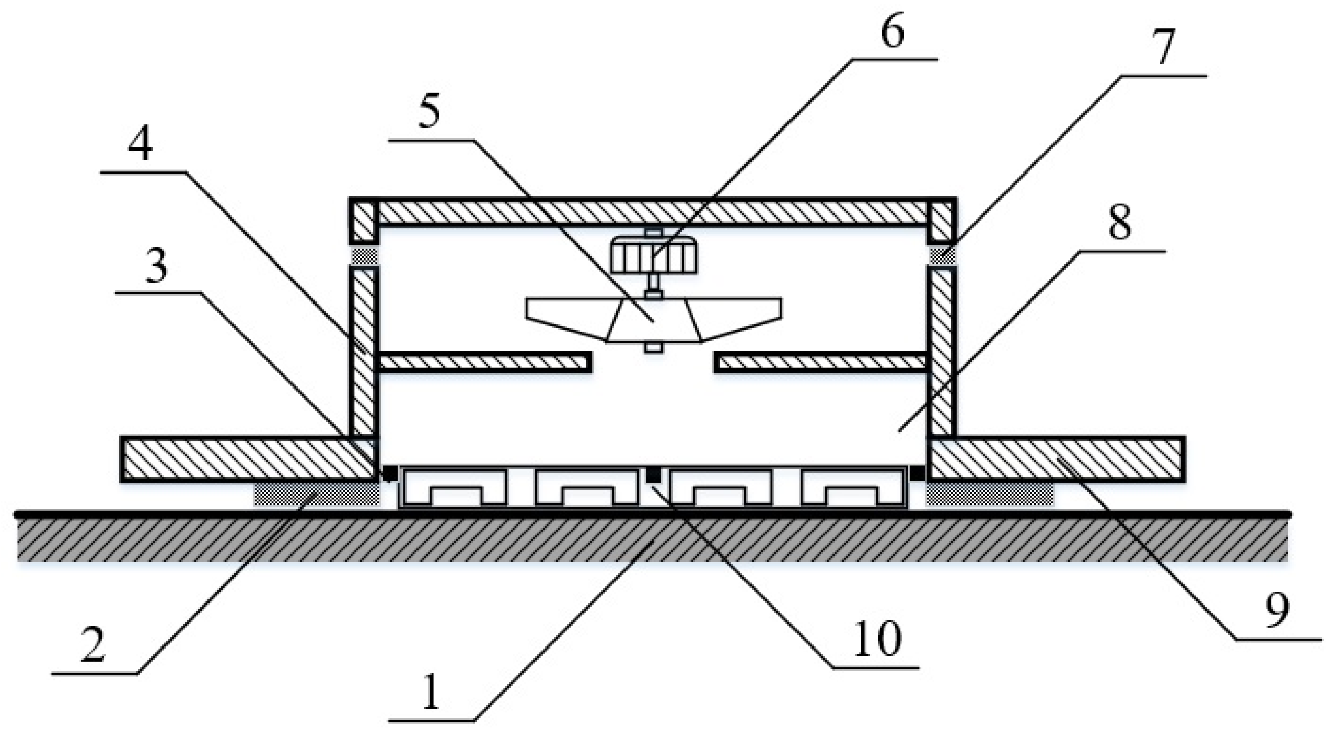
The designed length of the wall–climbing robot chassis is 0.8 m, and the width is 0.6 m. According to Figure 1, the coupling adsorption mechanism adopts an integrated design. The electromagnetic adsorption device is fixed to the lower part of the robot chassis and is nested and installed at the air inlet of the negative pressure adsorption mechanism. The diameter of the center ring of the electromagnetic array is 0.3 m, and the longitudinal diameter extends <0.05 m upward and downward. The structural conditions of the electromagnetic array determine that the shape of the negative pressure chamber is cylindrical, with an overall height of 0.2 m and an inlet radius of 0.2 m. A high–speed motor and a centrifugal fan are installed in the upper part of the negative pressure chamber, and a sealing device is connected to the lower part. The sealing device adopts a circular structure. Since the diameter of the outer ring of the sealing device shall not exceed the structural limit of the width of the robot chassis, the length of the sealing device is set to 0.1 m.

Calculated according to a design mass of the body and load of 30 Kg, without considering the electromagnetic adsorption force and under the premise of ensuring the safe adsorption of the wall–climbing robot, the negative pressure adsorption force required in the vertical motionless state is 327 N, and the negative pressure adsorption force required in the vertical motion is 393 N.

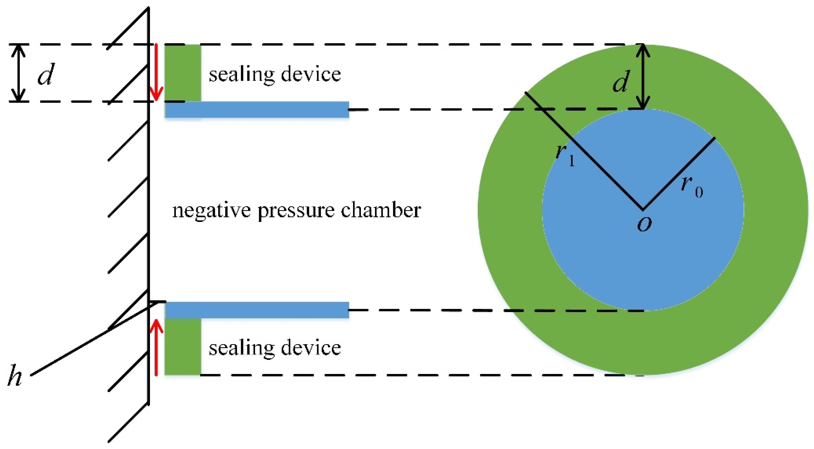
As illustrated in Figure 2, r₁ is the sum of the inlet radius of the vacuum cavity and the length of the sealing device. The negative pressure chamber and the sealing device have a pressure difference with the external atmosphere simultaneously, and they are subject to the normal thrust from the atmosphere. The equation of the action area of the negative pressure adsorption force is as follows:

$$S=\pi {(r_0+\frac{d}{2})}^2$$

(1)

Among which:

S—The action area of the negative pressure adsorption force;

r₀—Inlet radius of the negative pressure chamber, r₀ = 0.2 m;

d—Length of the sealing device, d = 0.1 m.

By calculating S = 0.1963 m², from the pressure formula, the minimum safe negative pressure in the two motion states of the robot is 1666 Pa and 2002 Pa, respectively. In the state of vertical motion, the output negative pressure of the wall–climbing robot is the highest negative pressure required by the system. At this time, the motion state of the air flow is used as the calculation standard for working conditions. Substituting the working condition point pressure difference Δp = 2002 Pa into the internal and external pressure difference formula of the sealing device,

$$\Delta p=\frac{\mu v^2}{d}+\frac{\rho v^3}{25}-2\rho v^2$$

(2)

Among which:

v—The main velocity of the air flow in the fluid channel (m/s);

ρ—The air density. At standard atmospheric pressure and at 20 °C, ρ = 1.205 kg/m³;

μ—The aerodynamic viscosity. At standard atmospheric pressure and at 20 °C, μ = 17.9 × 10⁻⁶ Pa·s.

The main velocity of the air flow in the fluid channel v = 61.11 m/s is calculated. Under the premise that the main velocity is fixed, the height of the fluid channel of the sealing device is

$$h=10\sqrt{\frac{\mu d}{\rho v}}$$

(3)

The channel height h = 0.0016 m corresponding to the critical pressure difference is calculated. According to the empirical formula, the flow rate of air flow under working conditions is

$$q_v=\frac{l{h}^3}{12\mu d}\Delta p$$

(4)

Among which:

h—Fluid channel height;

l—Length of the middle line of the sealing device, l = 2π (r₀ + d/2) = 1.5708 m.

Substitute the data and calculate q_v = 0.5548 m³. Based on the specific analysis of the structure of the experimental model of the negative pressure adsorption device and the fluid pneumatic parameters of the highest negative pressure operating condition point, the basic data and boundary values of the negative pressure adsorption experiment are obtained, as shown in

Table 1. Admission conditions for negative pressure adsorption experiment.

Admission Conditions	Value
Robot chassis dimension	0.8 × 0.6 (m)
Standard air pressure (environmental parameters)	1.01325 × 105 (Pa)
Air density (environmental parameters)	1.205 (kg/m3)
Gas temperature (environmental parameters)	20 °C
Maximum adsorption force of the system	393 (N)
Maximum negative pressure of the system	2002 (Pa)
Radius of negative pressure chamber	0.2 (m)
Cross–sectional area of negative pressure chamber	0.1257 (m2)
Negative pressure chamber length	0.2 (m)
Average flow rate of negative pressure chamber	<40.76 (m/s)
Reynolds number of fluid in negative pressure chamber	<103.85
Air flow	<0.6 (m3/s)
Sealing device length	0.1 (m)
Sealing device height	<0.0016 (m)
Main flow rate of Leakage channel	<61.11 (m/s)

.

(2)

Calculation of structural parameters of centrifugal fan

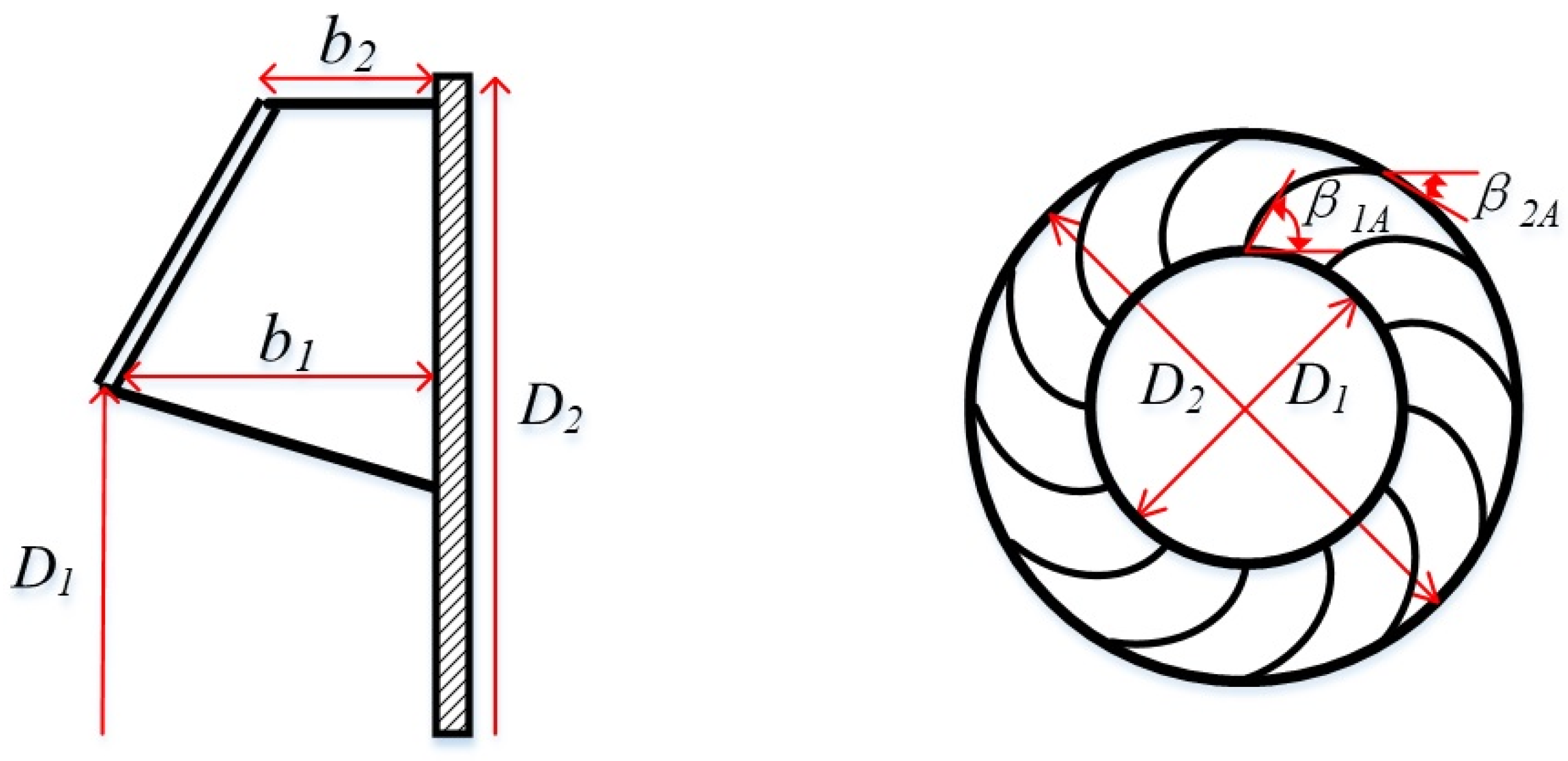
As the most important component of the robot’s negative pressure adsorption mechanism, the centrifugal fan is the negative pressure–generating device in the negative pressure chamber. The efficiency of the negative pressure adsorption device directly depends on the performance of the centrifugal fan. Through analysis of the entry conditions of the negative pressure adsorption experiment, and based on empirical formulas and parameter standards, the geometric dimensions of the fan impeller are calculated, including impeller inlet diameter D₁, impeller outlet diameter D₂, blade inlet width b₁, blade outlet width b₂, blade inlet mounting angle β_1A, blade outlet mounting angle β_2A, blade number Z, etc. [21,22], as illustrated in Figure 3.

The impeller of the centrifugal fan adopts a tapered front disc structure, and the blade profile adopts a backward–leaning design. There is no front axial impeller in front to adjust the air flow. There is no chassis at the rear, and the air flowing out of the air outlet directly merges with the atmosphere and is then discharged from the air outlet. In this working state, the full pressure of the centrifugal fan is equal to the static pressure at the inlet of the fan:

$$p_t=p_{s1}$$

(5)

Among which:

p_t—Centrifugal fan full pressure;

p_s1—Static pressure at the inlet of the fan, namely the negative pressure in the negative pressure chamber.

Drawing on the design experience of ventilation devices, the outlet angle β_2A of the impeller of the backward–leaning centrifugal fan has a greater influence on the dimension and performance of the fan. The recommended range of literature is between 30° and 50° [23]. To obtain higher full–pressure efficiency, β_2A = 30° is selected, the corresponding full pressure coefficient ψ = 0.8417, and the entrainment velocity v_2e of the air flow at the outlet of the centrifugal fan is

$$v_{2e}=\sqrt{\frac{2p_t}{\rho \psi }}$$

(6)

Among which:

ψ—the full pressure coefficient of the air flow.

Substitute the data and calculate, v_2e = 62.83 m/s. The outlet diameter D₂ of the fan impeller is not only positively related to the entrainment velocity of the fluid outlet, but also directly related to the fan speed n. The calculation equation is as follows:

$$D_2=\frac{60v_{2e}}{\pi n}$$

(7)

Among which:

n—The fan speed (r/min).

Under the conditions of structural space constraints, the value of the fan speed is adjusted several times for verification, and it is determined that the fan speed n = 4000 r/min and the outlet diameter D₂ = 0.31 m are convenient for calculation. Here, D₂ is set to 0.3 m.

To calculate the inlet diameter D₁ of the fan impeller, the flow coefficient φ of the air flow should be calculated first:

$$\phi =\frac{4q_v}{\pi D_2^2{v}_{2e}}$$

(8)

$$D_1=\left[(0.715\sim 1.01)k{D}_2\frac{{\phi }^{\frac{1}{2}}}{{\psi }^{\frac{1}{4}}}\right]$$

(9)

Among which:

φ—The flow coefficient of the air flow;

k—The scale factor for the smaller fan impeller of D₁, k = 1.5;

Substitute the data and calculate, φ = 0.1249, D₁ = 0.1235~0.1744 m. The inlet diameter D₁ is limited by the structural space as well, and the ratio to the outlet diameter D₂ should be set within a reasonable range. Synchronously, the flow coefficient φ and the full pressure coefficient ψ of the air flow also have a certain adjustment effect on the value of the inlet diameter D₁. To simplify the calculation, here, D₁ is set to 0.15 m.

Blade inlet width b₁ refers to the projection of the inlet edge curve of the fan impeller on the meridian surface. The value depends on the fluid flow through the centrifugal fan:

$$b_1=\frac{D_{{}_1}^2}{4D_{1c}\xi \mu }$$

(10)

Among which:

D_1c—Average value of inlet diameter (m);

ξ—Inlet area proportional coefficient, ξ = 0.7;

μ—Airflow filling coefficient before inlet. For tapered front plate, μ = 0.83~0.91.

Substitute the data and calculate, b₁ = 0.0595 m, which is in line with the system space requirements. To simplify the calculation, here, b₁ is set to 0.06 m. The value of the blade outlet width b₂ depends on D_1c, D₂ and b₁. The simplified empirical equation is

$$b_2=\frac{b_1}{k}\frac{D_{1c}}{D_2}$$

(11)

Among which:

k—Outlet outflow velocity coefficient, k = v*_2n/v_2n.

The variable k is a metric coefficient, and it represents the change in speed before and after the air flows out of the centrifugal fan. Variable v_2n represents the normal velocity of the corresponding vector diameter when the fluid reaches the edge of the blade and has not yet flowed out. Variable v*_2n represents the normal velocity of the corresponding vector diameter when the fluid has just flowed out of the fan blade.

Due to the difficulty of measuring and calculating the itemized speed of the air flow and according to the recommendations of the relevant literature, when the specific speed of the centrifugal fan is between 35 and 70, k = 0.7. Substitute the data and calculate, b₂ = 0.042 m. For convenience of calculation, b₂ is set to 0.04 m here.

Based on the principle of minimizing the relative speed of the inlet [24], the relevant literature calculates that the optimal solution of the inlet angle of the backward fan is 35.26°. Variable β_1A is set to 35° here.

In theory, the increase in the number of impeller blades is conducive to increasing the impeller pressure and reducing the influence of relative eddy currents on the air flow. Meanwhile, increasing the blades narrows the impeller fluid, increases friction loss, and reduces the total fan pressure. Therefore, it is essential to calculate the optimal number of blades for centrifugal fans:

$$Z=\tau \pi (\frac{D_2+D_1}{D_2-D_1})\sin (\frac{{\beta }_{1A}+{\beta }_{2A}}{2})$$

(12)

Among which:

τ—Cascade density, τ = 0.5 + 1.7β_2A;

Substitute the data and calculate, τ = 1.35, Z = 11.5314. For the convenience of marking, here, Z is set to 12.

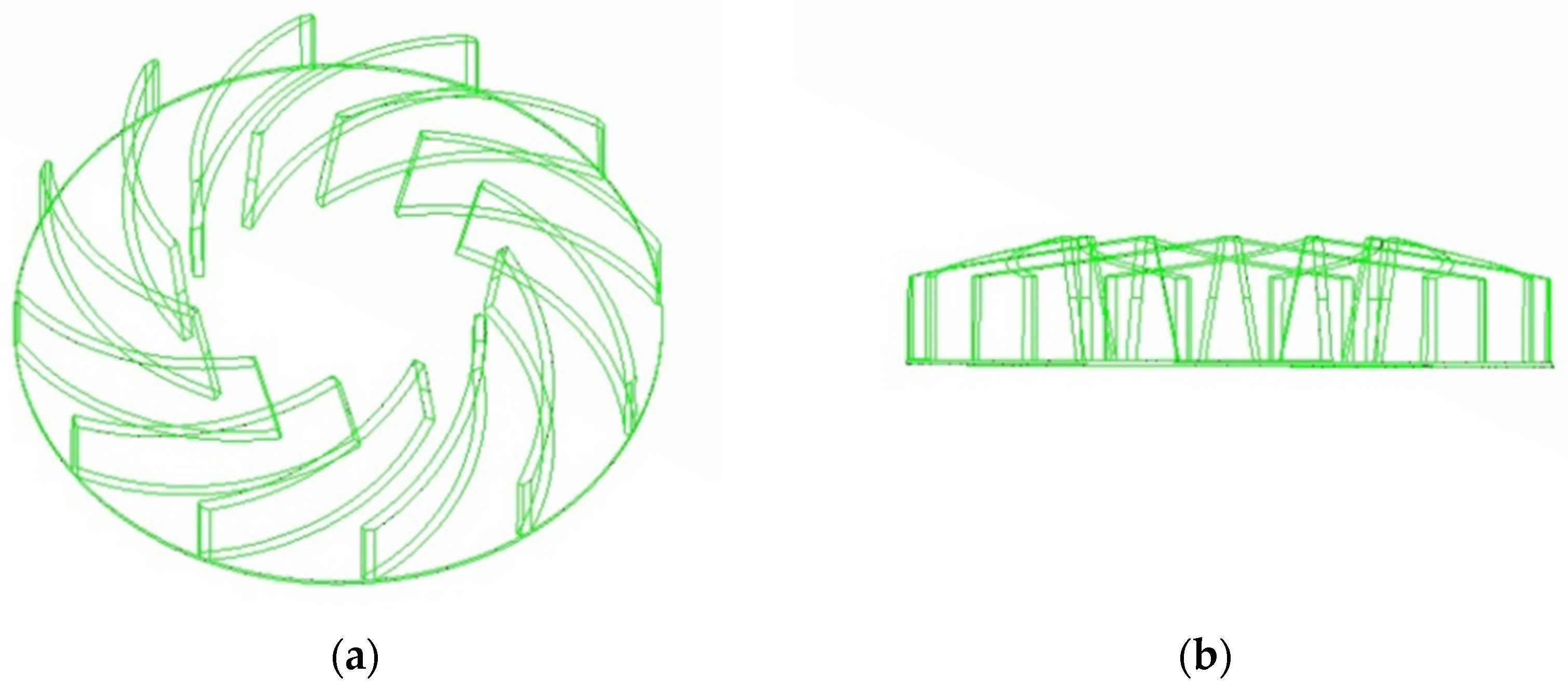
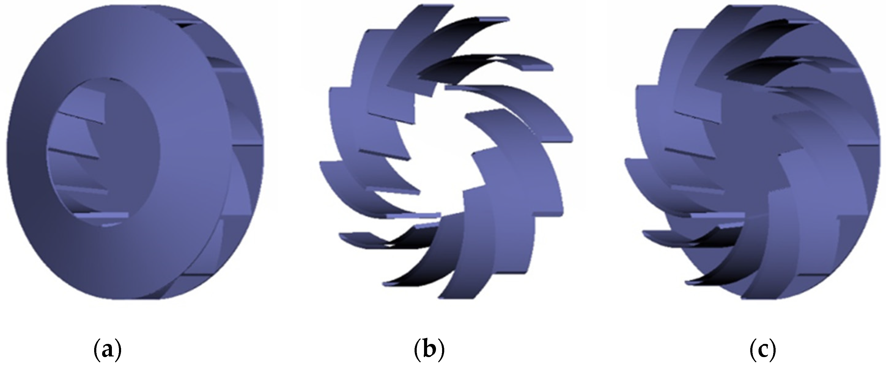
In the above, the structural parameters such as the geometry, installation angle, and number of blades of the centrifugal fan impeller are calculated. According to the structural calculation results, the impeller structure of the centrifugal fan is generated, as shown in Figure 4.

The calculation results of the structural parameters of the centrifugal fan are summarized in

Table 2. Centrifugal fan impeller structure parameters.

Geometric Parameter	Value
Impeller inlet diameter (average value)	0.149 (m)
Impeller inlet diameter	0.15 (m)
Impeller outlet diameter	0.3 (m)
Blade inlet width	0.06 (m)
Blade outlet width	0.04 (m)
Blade inlet mounting angle	35o
Blade outlet mounting angle	30o
Cascade density	1.35
Number of blades	12
Blade thickness	0.005 (m)
Specific speed	57.35
Fan speed	4000 r/min
low coefficient	0.1249
Full pressure coefficient	0.8417
Inlet area proportional coefficient	0.7
Airflow filling Coefficient before inlet	0.9
Outlet outflow velocity coefficient	0.7
Circulation coefficient	0.8643
Theoretical fan full pressure	2712 (Pa)
Calculated full fan pressure Actual fan full pressure	2350 (Pa) 2074 (Pa)

.

3. Negative Pressure Chamber Control Volume Fluid Field Experiment

Following the requirements of the experimental purpose, the negative pressure chamber control volume experiment aims to investigate the variations in the pressure distribution, fluid flow, and fluid velocity of the air flow in the sealing device and the negative pressure chamber during the continuous change in the negative pressure of the system in the negative pressure chamber. According to the experimental design, sub–experiments are carried out according to the pressure difference between the internal and external pressure of the negative pressure device. The design differential pressure, denoted as Δp, is set to 500 Pa, 1000 Pa, 1500 Pa, and 2000 Pa, respectively. The structure model of the negative pressure chamber control volume is shown in Figure 5.

(1)

Analysis of experimental results of fluid channel inspection surface

The intermediate height value of the fluid channel of the sealing device is selected to establish the inspection surface. Parallel to the surface of the sealing device and the shaft lining, the inspection surface is located between the two, and its purpose is to investigate the movement state of the air flow in the fluid channel of the sealing device before entering the negative pressure chamber.

As shown in Figure 6, the legend view of the Δp = 2000 sub–experiment is used as a reference. In each sub–experiment, the color of the edge of the outer ring of the sealing device is the same, indicating that the gas pressure is not much different from the atmospheric pressure outside the channel in the initial stage of the air flow entering the fluid channel. With the continuous flow of air flow in the channel, the gas pressure gradually increases, reaching the maximum value at the inner edge of the fluid channel, which is numerically equal to the average negative pressure in the negative pressure chamber—namely, the set value of the negative pressure of the system. After the air flow enters the negative pressure chamber, the suction effect of the centrifugal fan on the rear side of the negative pressure chamber changes the direction of movement of the air flow from the horizontal movement to the vertical movement, resulting in a decrease in the horizontal gas pressure. In the pressure cloud diagram, it is manifested as the pressure of the annular area near the center of the circle at the inner edge of the channel is less than the pressure of the annular area near the circumference at the inner edge of the channel.

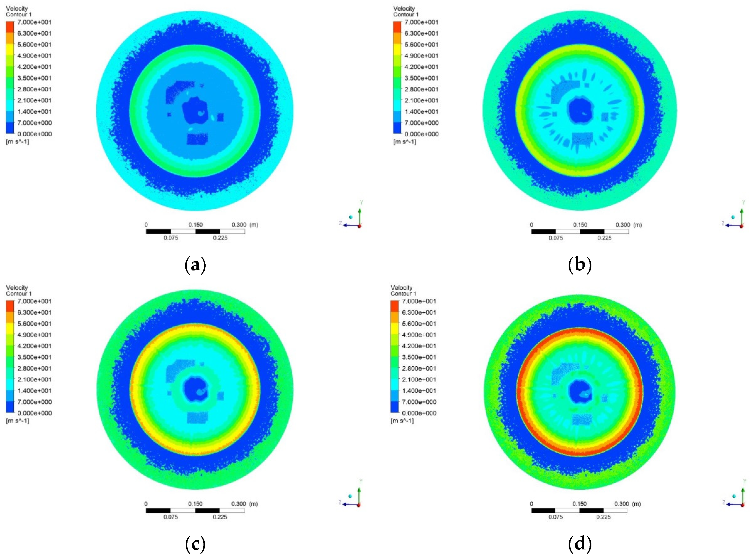
The legend range view is 0 m/s~70 m/s in Figure 7. Based on the figure, since the air flow pressure on the inside of the channel is directly affected by the change in the pressure of the negative pressure chamber, the fluid velocity on both sides of the channel in the fluid channel is greater than the fluid velocity in the middle of the channel, and the fluid velocity on the inside of the channel is greater than the fluid velocity on the outside of the channel. The pressure of the air flow on the outside of the channel is directly affected by the atmospheric pressure, and the gas pressure decreases faster during the fluid movement. However, compared with the air flow on both sides of the channel, the air flow in the middle of the channel has a pressure buffer at a certain distance, due to which the gas pressure does not change much, resulting in a lower fluid velocity. From the figure, it is also found that the inlet speed and outlet speed of the air flow in the fluid channel are directly affected by the negative pressure of the system. The greater the pressure difference between the inside and outside of the adsorption device, the greater the inlet speed and outlet speed of the air flow in the channel.

(2)

Analysis of the experimental results of the inspection surface of the negative pressure chamber

The intermediate value of the length of the negative pressure chamber is selected to establish the inspection surface. Parallel to the cross–section of the sealing device and the front plate of the centrifugal fan, the inspection surface is located between the two, mainly to investigate the horizontal movement state of the air flow after entering the negative pressure chamber.

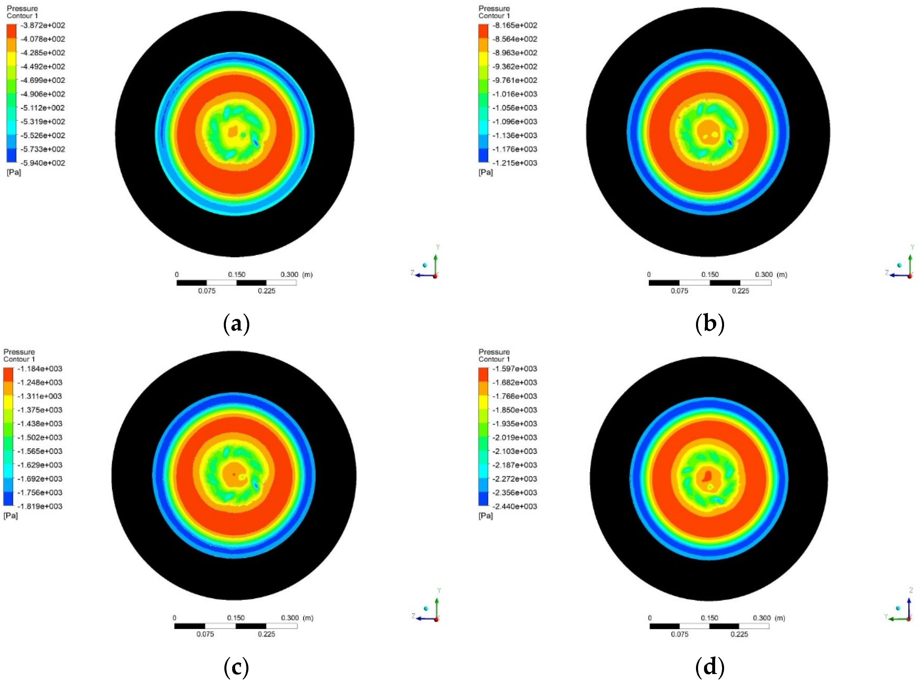
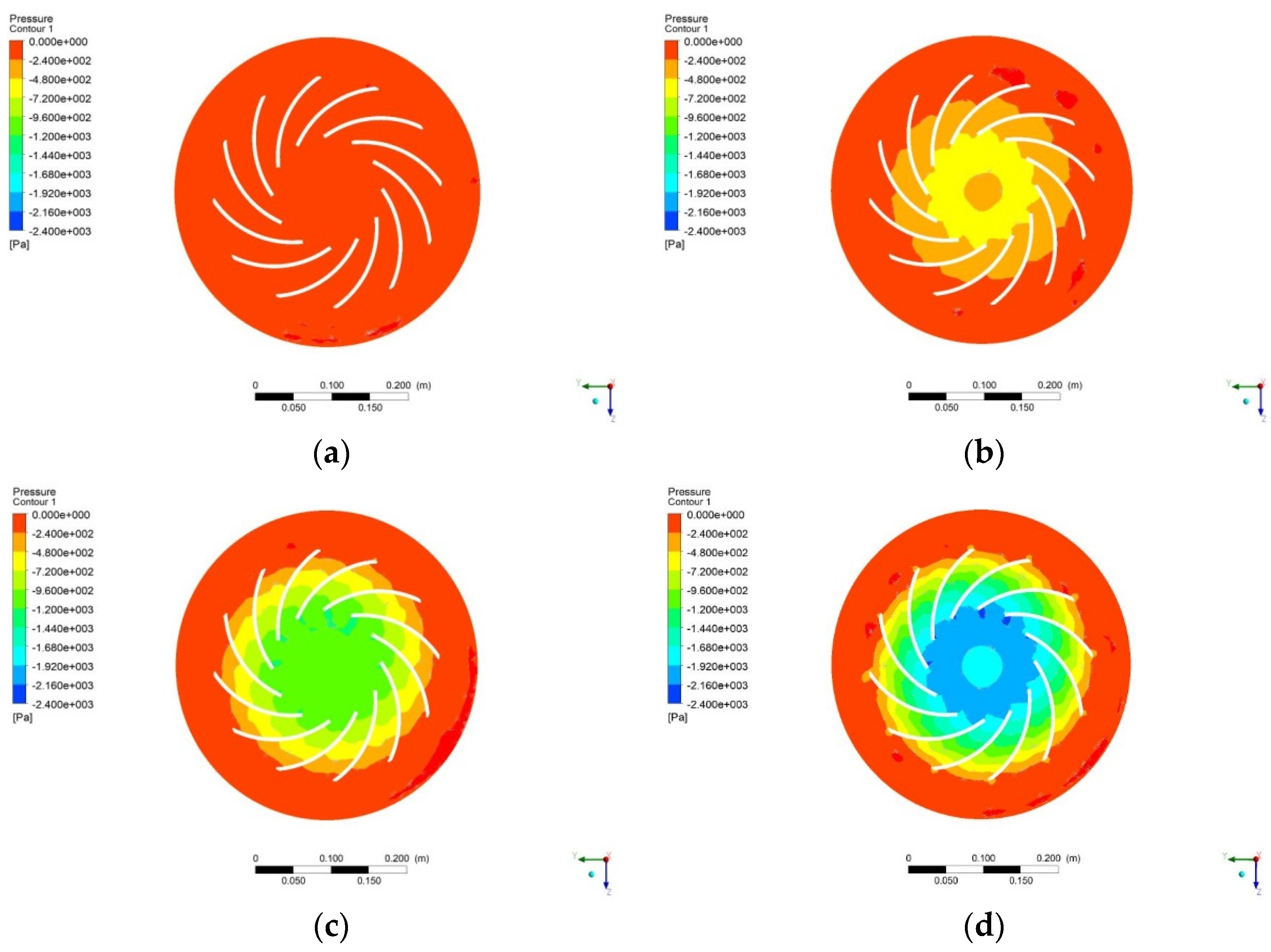
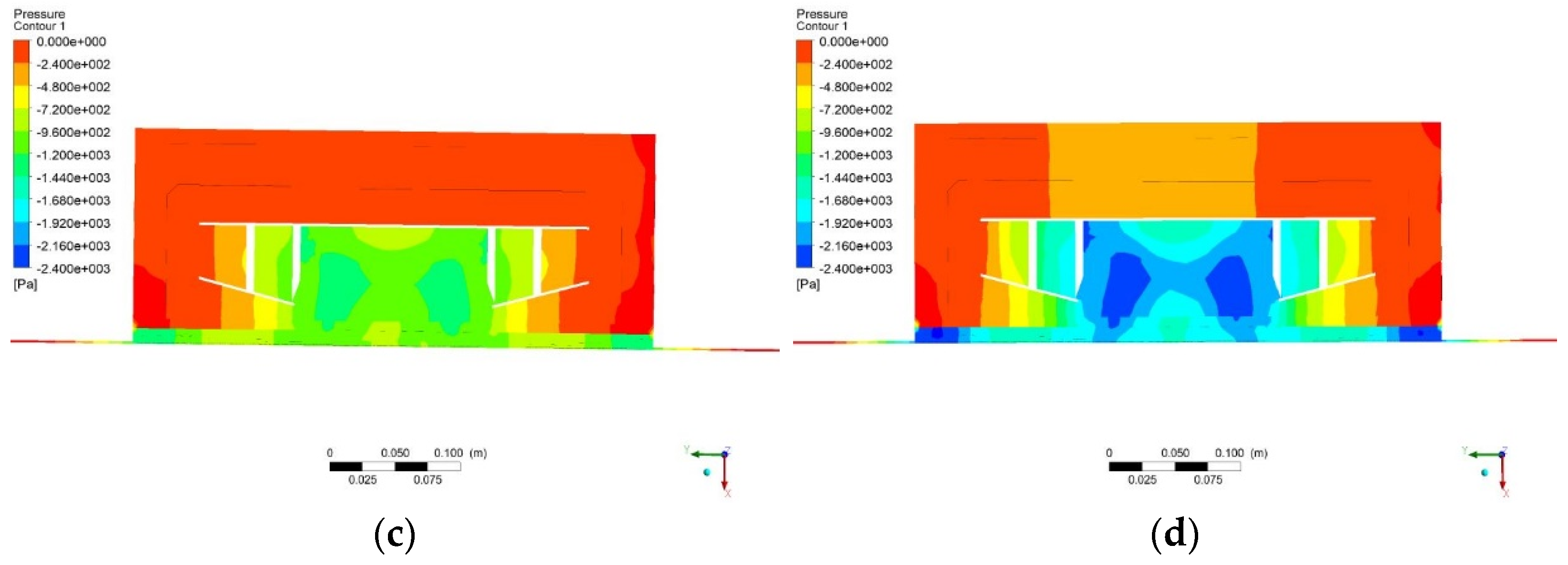
In Figure 8, at Δp = 500, the pressure range is −594 Pa~−387 Pa; at Δp = 1000, the pressure range is −1215 Pa~−817 Pa; at Δp = 1500, the pressure range is −1819 Pa~−1184 Pa; and at Δp = 2000, the pressure range is 2440 Pa~−1597 Pa. Observing the pressure distribution in the figure, it is found that in the transverse extension area of the negative pressure chamber, the pressure of the air flowing into the negative pressure chamber from the fluid channel is relatively high, so accordingly, the gas pressure in this area is relatively high. Subsequently, during the movement of the air flow to the center of the negative pressure chamber, the direction of fluid movement gradually changes from horizontal to vertical due to the influence of the suction force of the centrifugal fan, thereby decreasing the air pressure on the transverse surface of the negative pressure chamber gradually. In the central area of the negative pressure chamber, the suction power of the centrifugal fan dominates the direction of movement of the air flow. The vertical speed of the air flow increases rapidly, causing a certain increase in the gas pressure in this area.

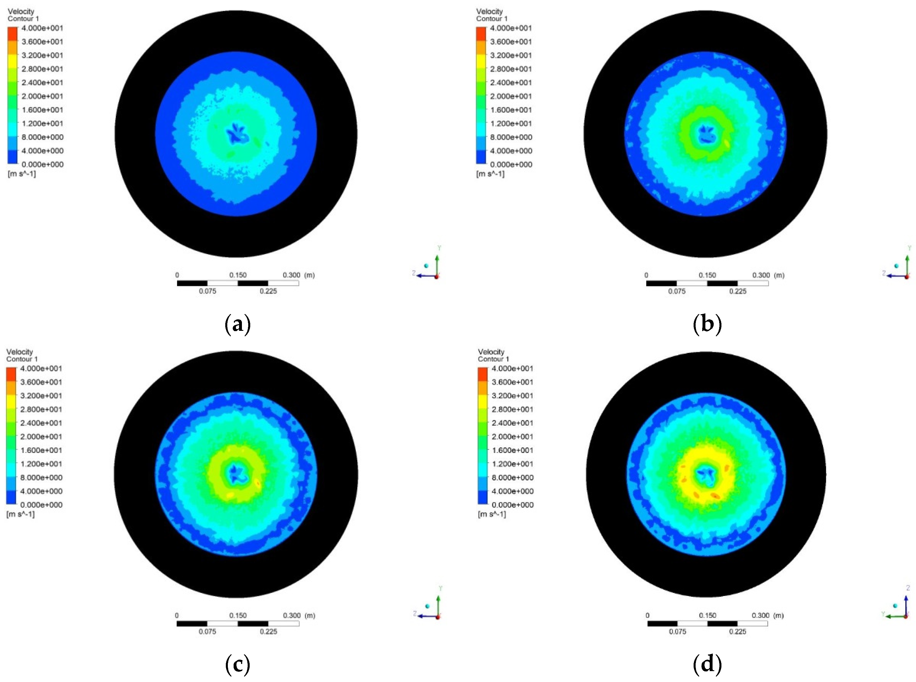
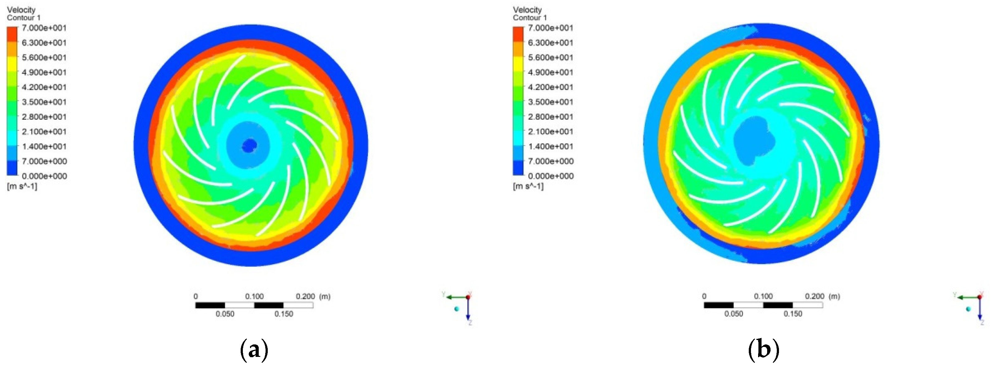
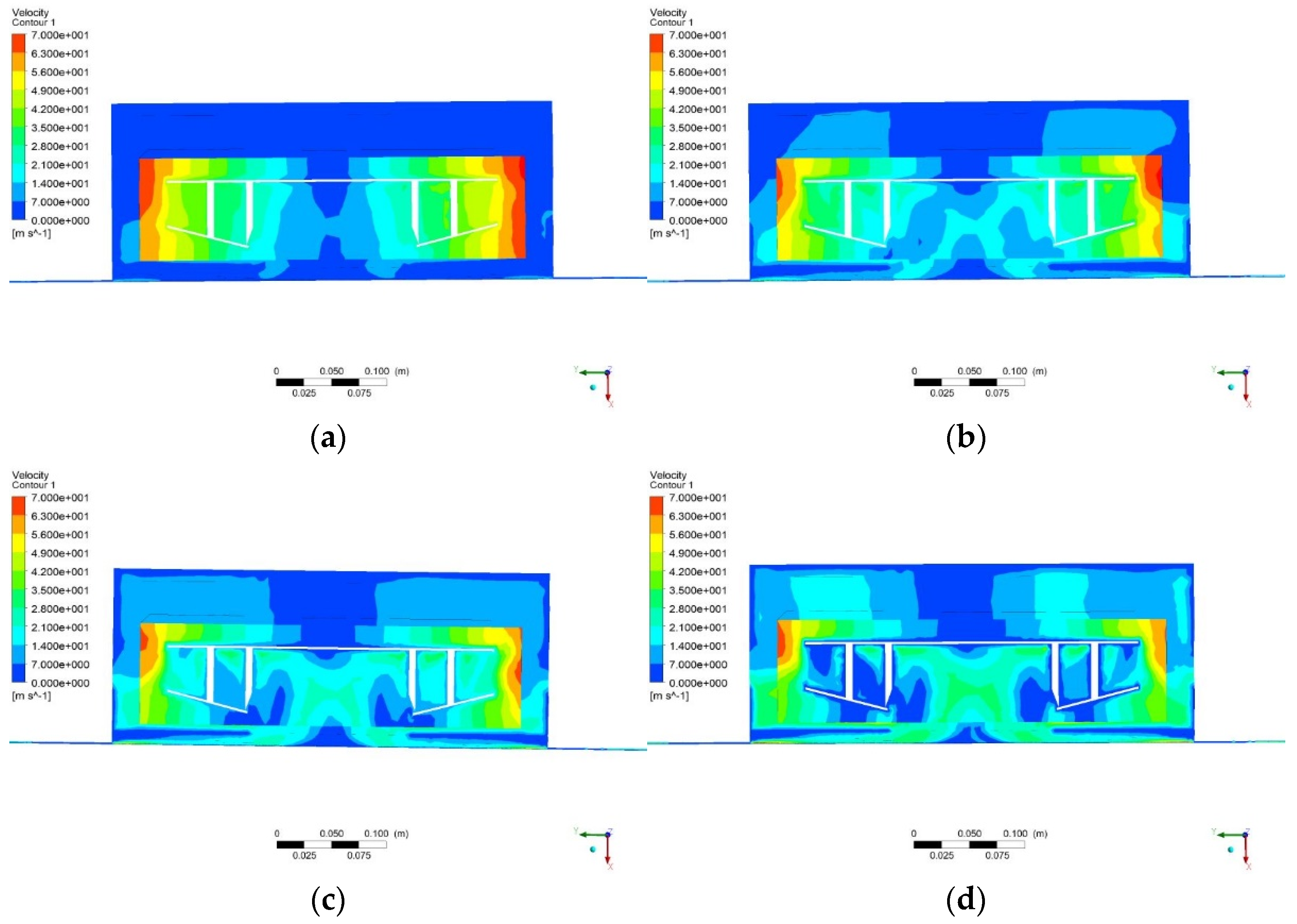
The legend range of legend view is 0 m/s~40 m/s in Figure 9. At the working condition points of Δp = 500 and Δp = 1000, after the air flow enters the negative pressure chamber through the fluid channel, its transverse velocity is basically reduced to near 0 m/s. At the working condition points of Δp = 1500 and Δp = 2000, under the same circumstances, the air flow can maintain a transverse inertial speed of 4 m/s~8 m/s, and then it drops to about 0 m/s, indicating that in the fluid channel of the sealing device, the direction of movement of the air flow and the main velocity depend on the internal and external pressure difference of the negative pressure adsorption mechanism. The greater the internal and external pressure difference, the greater the velocity of the fluid entering the negative pressure chamber. After the air flow enters the negative pressure chamber, the average pressure of the gas in the negative pressure chamber is the same as the pressure of the incoming gas, causing the incoming gas to lose differential pressure power, and the fluid velocity drops rapidly. Inside the negative pressure chamber, the direction of movement of the air flow and the main velocity depend on the speed of the centrifugal fan. In the negative pressure chamber, the air flow that has slowed to 0 m/s in the transverse direction is turned by the suction force of the centrifugal fan to the inlet of the centrifugal fan. The faster the speed of the centrifugal fan, the faster the vertical speed of the air flow entering the inlet of the centrifugal fan and thus the higher the negative pressure in the negative pressure chamber.

(3)

Numerical analysis of experimental data

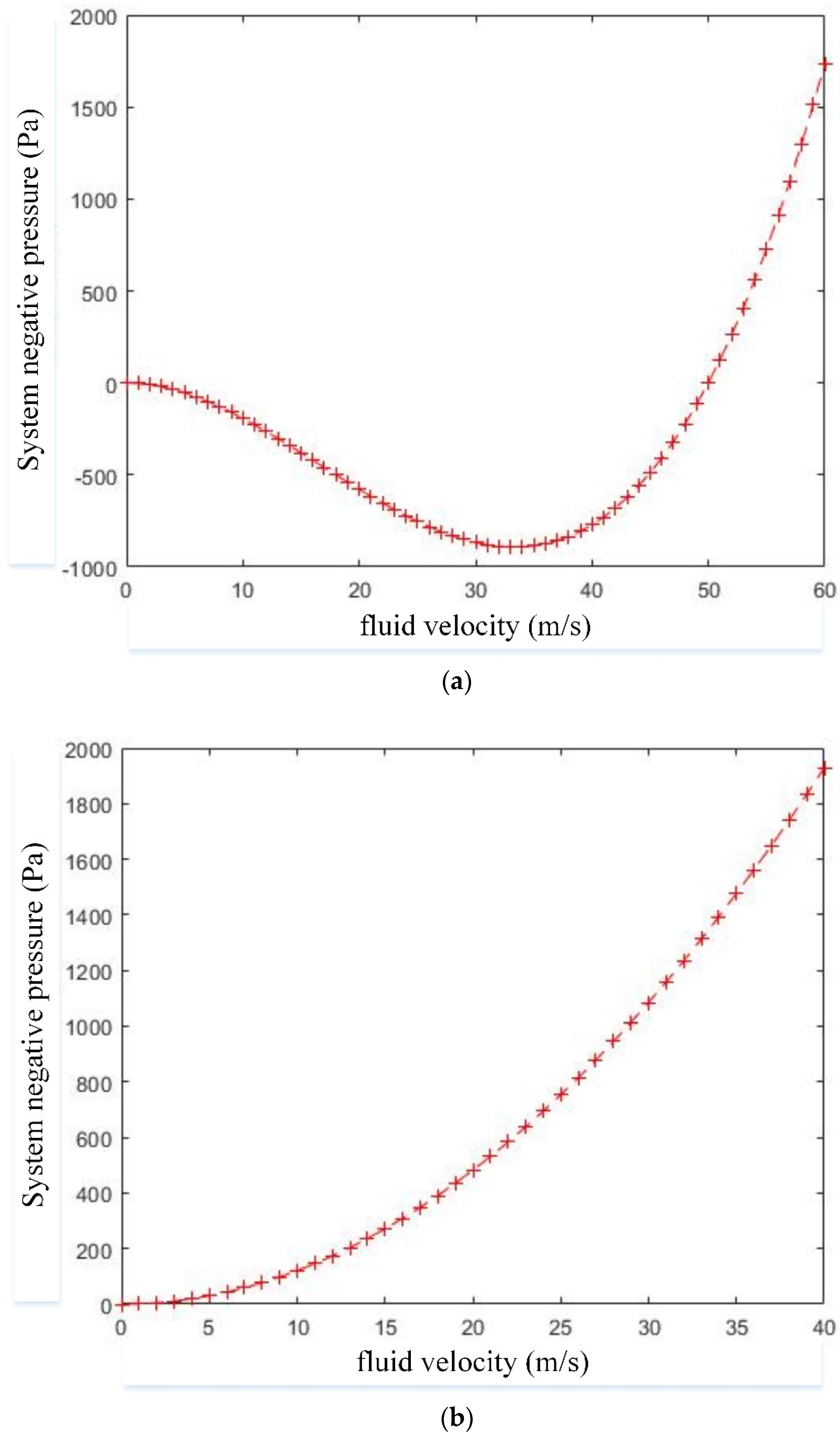
The corresponding Figure 9a of the internal and external pressure difference of the sealing device and the air velocity of the fluid channel is shown in Figure 10a. It has been observed that in the range of the fluid velocity <50 m³/s interval, the internal and external pressure difference of the sealing device is numerically negative; therefore, the system’s negative pressure value in this interval does not have any practical significance. In the fluid velocity range of 50~60 m³/s, the pressure difference between the inside and the outside of the sealing device is increased from 0 to 1735 Pa. The corresponding curve of the negative pressure in the negative pressure chamber and the air velocity in the chamber is shown in Figure 10b. The movement process of the air flow in the negative pressure chamber is relatively simple, and the movement stroke is relatively short. In the fluid velocity range of 0~40 m³/s, the pressure difference between the inside and the outside of the sealing device is increased from 0 to 1928 Pa. On the basis of the comprehensive analysis of the corresponding curve representing the negative pressure of the system and the sealing device and the flow rate of the air flow in the negative pressure chamber, the calculated value conforms to the expected result of the negative pressure system. In the process of pressure boost, the curve is smooth, and the negative pressure parameters do not fluctuate up and down, which is convenient for reducing the difficulty of controlling the negative pressure adjustment of the mechanism in the later stage. The experimental numerical calculation results can be found in Appendix A

Table A1. Simulation values of air flow parameters of sealing device and negative pressure chamber.

Negative Pressure Chamber			Sealing Device
System Negative Pressure (Pa)	Adsorption Pressure (N)	Fluid Velocity (m3/s)	Fluid Flow (m3)	Fluid Velocity (m3/s)	Device Height (mm)
100	19.64	9.1098	0.0366	50.7998	1.7104
200	39.27	12.8831	0.0715	51.5569	1.6974
300	58.90	15.7786	0.1051	52.2736	1.6858
400	78.54	18.2195	0.1374	52.9552	1.6748
500	98.17	20.3700	0.1686	53.6058	1.6646
600	117.81	22.3142	0.1989	54.2288	1.6551
700	137.45	24.1021	0.2283	54.8271	1.6460
800	157.08	25.7663	0.2569	55.4031	1.6375
900	176.71	27.3293	0.2847	55.9588	1.6293
1000	196.35	28.8076	0.3118	56.4959	1.6215
1100	215.98	30.2136	0.3383	57.0161	1.6141
1200	235.62	31.5571	0.3642	57.5205	1.6070
1300	255.25	32.8457	0.3895	58.0105	1.6002
1400	274.89	34.0856	0.4143	58.4869	1.5936
1500	294.52	35.2819	0.4388	58.9508	1.5874
1600	314.16	36.4390	0.4627	59.4030	1.5814
1700	333.79	37.5605	0.4863	59.8441	1.5756
1800	353.43	38.6494	0.5093	60.2749	1.5699
1900	373.06	39.7085	0.5320	60.6959	1.5644
2000	392.70	40.7400	0.5543	61.1078	1.5591

.

4. Centrifugal Fan Control Volume Fluid Field Experiment

According to the requirements of the experimental purpose, the purpose of the centrifugal fan control volume experiment is to investigate the ability of the centrifugal fan to adjust the static pressure of the inlet and outlet by adjusting the motor speed and the changes in the important pneumatic parameters of the air flow inside the control volume during fan speed changes. Experimental design and sub–experiments are carried out according to the speed of the centrifugal fan. The design speed n is 1000 r/min, 2000 r/min, 3000 r/min, and 4000 r/min, respectively. The structure model of the centrifugal fan control volume is shown in Figure 11.

(1)

Analysis of the experimental results of the horizontal inspection surface of the centrifugal fan

The intermediate value of the length of the centrifugal fan is selected to establish the inspection surface. Parallel to the front plate of the fan and the rear plate of the fan, the inspection surface is located in the middle of the longitudinal length of the impeller, which mainly investigates the horizontal movement state of the air flow after entering the centrifugal fan.

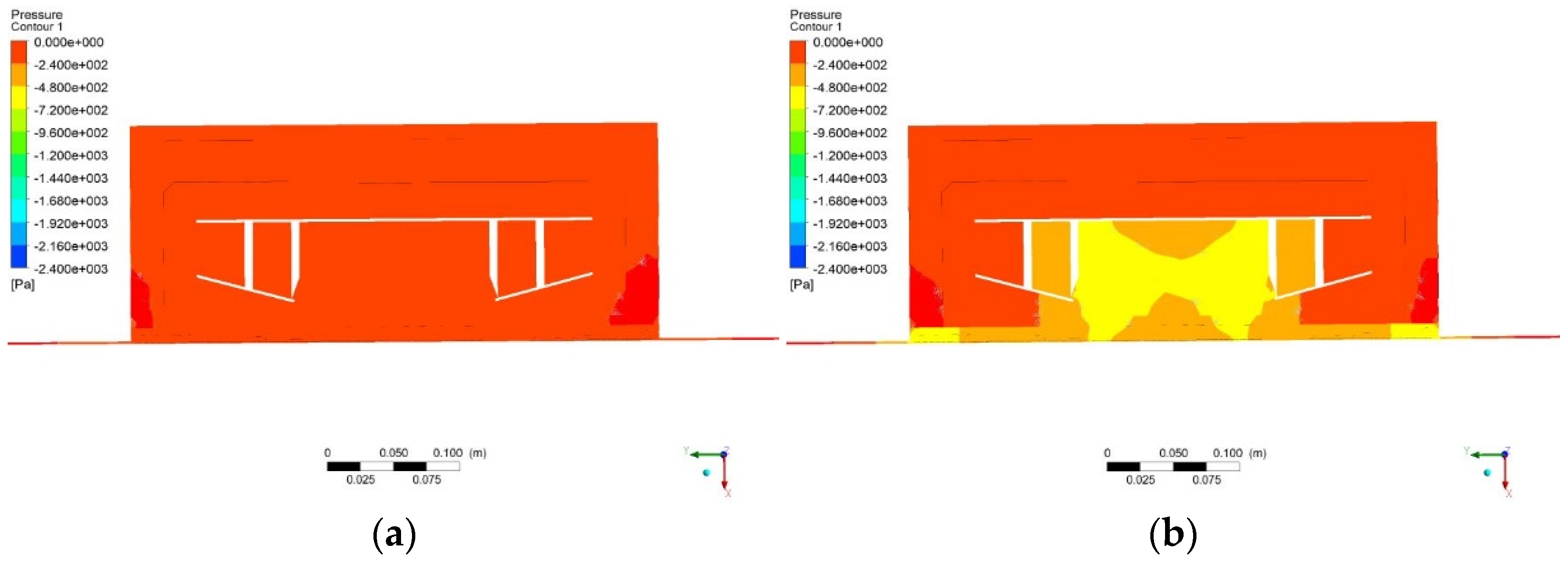
The legend range view is −2400 Pa~0 Pa in Figure 11. The inlet static pressure corresponding to the fan speed of each sub–experiment is as follows: at n = 1000 r/min, P_s1 = 125 Pa; at n = 2000 r/min, P_s1 = 500 Pa; at n = 3000 r/min, P_s1 = 1126 Pa; and at n = 4000 r/min, P_s1 = 2002 Pa. It can be observed from the figure that when the centrifugal fan speed is low, the inlet static pressure formed by the fan rotation is small, resulting in a small overall pressure gradient, and the pressure distribution shown in the pressure cloud diagram is not obvious. As the fan speed increases, both the static pressure at the fan inlet and the overall pressure gradient continue to increase, making the fluid pressure distribution depicted in the pressure cloud map more prominent. As shown in Figure 12d, the fluid pressure value at the inlet of the fan is the largest. Subsequently, due to the change in the direction of movement of the air flow between the fan blades, the fluid pressure decreases gradually until it is thrown out by the blades and merges with the external atmosphere at the air outlet, thereby, the fluid pressure returning to the standard atmospheric pressure.

The legend range of legend view is 0 m/s~70 m/s in Figure 12. At speed n = 1000 r/min, as shown in Figure 13a, the fan speed is low, and the overall speed gradient is distributed in a ring, gradually increasing from the center of the fan to the radial direction until the maximum value is reached at the outlet of the fan. At n = 2000 r/min, as displayed in Figure 13b, as the fan speed increases, the fluid velocity distribution has a more obvious velocity separation phenomenon, and the fluid velocity close to the front blade is gradually smaller than the fluid velocity close to the rear blade. At n = 3000 r/min, as illustrated in Figure 13c, due to the continuous increase in fan speed, the circular distribution trend of the overall speed gradient can no longer be observed from the speed cloud map, and the speed separation phenomenon of the air flow in the middle of the blade is more obvious. At n = 4000 r/min, as shown in Figure 13d, since the fan speed reaches the maximum value of the operating condition point, in the area close to the front blade, a large low–speed area is formed along the direction of the fluid movement, and the fluid speed is significantly smaller than the fluid speed in the area close to the rear blade.

(2)

Analysis of the experimental results of the longitudinal inspection surface of the centrifugal fan

The tangential direction of the diameter of the centrifugal fan is selected to establish the inspection surface. Perpendicular to the horizontal inspection surface of the centrifugal fan, the inspection surface is in the cross–sectional diameter of the negative pressure chamber, which is designed to investigate the longitudinal movement state of the air flow after entering the centrifugal fan.

In Figure 14, legend view is set to −2400 Pa~0 Pa. In each sub–experiment, the gas pressure at the edge of the negative pressure chamber and at the inlet of the centrifugal fan is large, which is numerically close to the negative pressure of the system at the working condition point. The air pressure in the fluid transition area and the front–end area of the fan is small, which is mainly due to the small design length of the negative pressure chamber. After passing through the fluid channel, the air flow with higher pressure enters the negative pressure chamber; because there is no longitudinal flow interval, it can only flow horizontally according to the inertial speed. Throughout this process, the inertial velocity of the air flow is consumed continuously, and the horizontal flow velocity decreases, causing the gas pressure to decrease. At the inlet of the centrifugal fan, and under the action of the suction force of the centrifugal fan, the movement speed of the air flow accelerates and the gas pressure increases. At the front end of the centrifugal fan, a certain eddy current formed by the air flow in this area causes the speed of the air flow here to decrease. Therefore, the gas pressure is lower than the gas pressure at the inlet of the centrifugal fan.

The legend range view is 0 m/s~70 m/s in Figure 15. According to the figure, on the side of the negative pressure chamber of the front plate of the centrifugal fan, the speed of the air flow has basically approached 0 m/s. The greater the differential pressure, the thinner the zeroing velocity layer. Meanwhile, the thicker the transition speed layer, the greater the negative pressure demand of the system and the higher the speed of the centrifugal fan adjustment, which in turn produces greater suction power to make the air flow at a higher speed. It is observed that the fluid velocity rises slowly in the middle channel of the blade and rises faster after flowing out of the fan, suggesting that the air flow is affected by the blade profile during the movement of the blade channel. The direction of fluid movement is not in a straight line; it is in a curved line in accordance with the blade profile. The development of fluid velocity is limited by the separation of velocity during movement.

(3)

Numerical analysis of experimental data

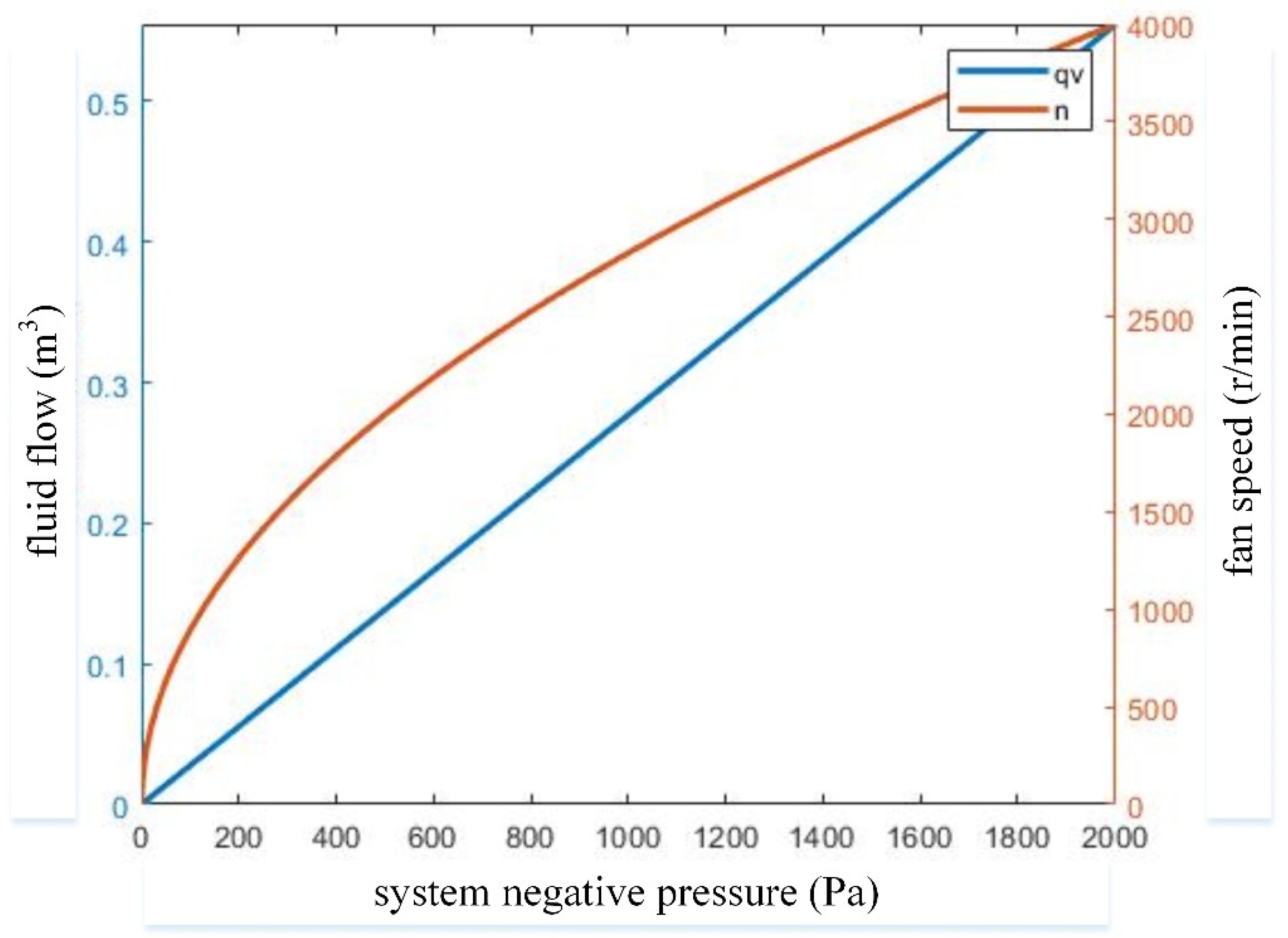
The curve corresponding to the negative pressure of the system between the flow rate of the air flow and the fan speed during the movement of the centrifugal fan control volume is shown in Figure 16. From the curve in the figure, it can be seen that the three pneumatic parameters of the air flow are positive linear relationship hips, and their respective numerical boundaries are consistent with the simulation results. Under the premise of determining the values of other parameters, the height of the fluid channel has a very subtle impact on the negative pressure and gas flow of the system, and the size of the fluid flow is mainly determined by the negative pressure required by the system. At the same time, in the initial stage of the system’s negative pressure and gas flow increase, the fan speed increases faster. When the immediate speed reaches 1/2 of the boundary speed, that is, after 2000 r/min, the speed curve flattens, and the slope of the curve gradually decreases. At this time, the negative pressure value of the system is 500 Pa, and the gas flow rate is 0.1387 m³, which are all at 1/4 of the boundary of their respective values, indicating the initial stage of the start of the centrifugal fan. The negative pressure adsorption mechanism has to output more power to increase the fan speed, making the system loss increase. In the process of speeding up the fan from the intermediate speed to the boundary speed, the year–on–year increase in the negative pressure and gas flow of the system is large, and a better operating efficiency is obtained by the negative pressure adsorption mechanism. The experimental numerical calculation results can be found in Appendix A 

Table A2. Simulation values of fluid velocity components of centrifugal fans.

Fan Speed (r/min)	Inlet Velocity Component (m/s)			Outlet Velocity Component (m/s)
	v1	v1e	v1r	v2	v2e	v2r
100	0.0397	0.0567	0.0693	0.9069	1.5708	1.8138
200	0.1040	0.1485	0.1813	1.8138	3.1416	3.6276
300	0.1928	0.2753	0.3361	2.7207	4.7124	5.4414
400	0.3061	0.4371	0.5336	3.6276	6.2832	7.2552
500	0.4439	0.6340	0.7739	4.5345	7.8540	9.0690
600	0.6063	0.8659	1.0570	5.4414	9.4248	10.8828
700	0.7932	1.1328	1.3829	6.3483	10.9956	12.6966
800	1.0046	1.4347	1.7515	7.2552	12.5664	14.5104
900	1.2406	1.7717	2.1629	8.1621	14.1372	16.3242
1000	1.5011	2.1437	2.6170	9.0690	15.7080	18.1380
1100	1.7861	2.5508	3.1139	9.9759	17.2788	19.9518
1200	2.0956	2.9929	3.6536	10.8828	18.8496	21.7656
1300	2.4297	3.4700	4.2361	11.7897	20.4204	23.5794
1400	2.7883	3.9822	4.8613	12.6966	21.9911	25.3932
1500	3.1715	4.5293	5.5293	13.6035	23.5619	27.2070
1600	3.5791	5.1116	6.2401	14.5104	25.1327	29.0208
1700	4.0114	5.7288	6.9936	15.4173	26.7035	30.8346
1800	4.4681	6.3811	7.7899	16.3242	28.2743	32.6484
1900	4.9493	7.0684	8.6289	17.2311	29.8451	34.4622
2000	5.4551	7.7907	9.5107	18.1380	31.4159	36.2760
2100	5.9855	8.5481	10.4353	19.0449	32.9867	38.0898
2200	6.5403	9.3405	11.4027	19.9518	34.5575	39.9036
2300	7.1197	10.1680	12.4128	20.8587	36.1283	41.7174
2400	7.7236	11.0305	13.4657	21.7656	37.6991	43.5312
2500	8.3521	11.9280	14.5614	22.6725	39.2699	45.3450
2600	9.0050	12.8605	15.6998	23.5794	40.8407	47.1588
2700	9.6825	13.8281	16.8810	24.4863	42.4115	48.9726
2800	10.3846	14.8307	18.1050	25.3932	43.9823	50.7864
2900	11.1111	15.8684	19.3717	26.3001	45.5531	52.6002
3000	11.8622	16.9410	20.6812	27.2070	47.1239	54.4140
3100	12.6379	18.0487	22.0334	28.1139	48.6947	56.2278
3200	13.4380	19.1915	23.4285	29.0208	50.2655	58.0416
3300	14.2627	20.3692	24.8663	29.9277	51.8363	59.8554
3400	15.1119	21.5821	26.3468	30.8346	53.4071	61.6692
3500	15.9857	22.8299	27.8702	31.7415	54.9779	63.4830
3600	16.8839	24.1128	29.4362	32.6484	56.5487	65.2968
3700	17.8067	25.4307	31.0451	33.5553	58.1195	67.1106
3800	18.7541	26.7836	32.6967	34.4622	59.6903	68.9244
3900	19.7259	28.1716	34.3911	35.3691	61.2611	70.7382
4000	20.7223	29.5946	36.1283	36.2760	62.8319	72.5520

.

5. Electromagnetic Field Experiment of Electromagnetic Adsorption Device

The purpose of the electromagnetic field experiment is to investigate the changes in electromagnetic suction and magnetic field parameters under different adsorption conditions between the electromagnetic unit and the reinforcement bar of the shaft lining during the movement of the wall–climbing robot. In the sub–experiment, the model of the reinforcement bar model and the corresponding angle to the electromagnetic unit and the input current of the wire coil are adjusted in turn, and the changes in electromagnetic adsorption force, magnetic flux density, magnetic field strength, adsorption area and electric field strength are analyzed. The experimental model of the electromagnetic adsorption device is illustrated in Figure 17.

In Figure 17, the winding coil is modeled as a whole. The current module is designed to guide the current input direction. The material properties of the unit iron core and reinforcement bar model are defined as steel–like materials. The relative permeability is set to 43,372 and 8000, respectively, and the conductivity is set to 2 MS/m; the material properties of the winding coil are selected as copper. The default relative permeability in the component library is set to 0.999991, and the conductivity is set to 58 MS/m. The material attribute of the gap filling is set to vacuum air, the relative permeability is set to 1, and the conductivity is set to 0 MS/m. In the sub–experiments where current changes are excluded, the excitation current value is set to 1950 (N × I).

The intermediate value of the side width of the electromagnetic unit and the intermediate value of the end face width are selected to establish two inspection surfaces perpendicular to each other in the horizontal and vertical directions. The intensity distribution and direction of movement of the magnetic flux inside the model under different states of electromagnetic adsorption between the electromagnetic unit and the reinforcement bar in the wall, as well as the change in electromagnetic adsorption force with the experimental variables, are analyzed.

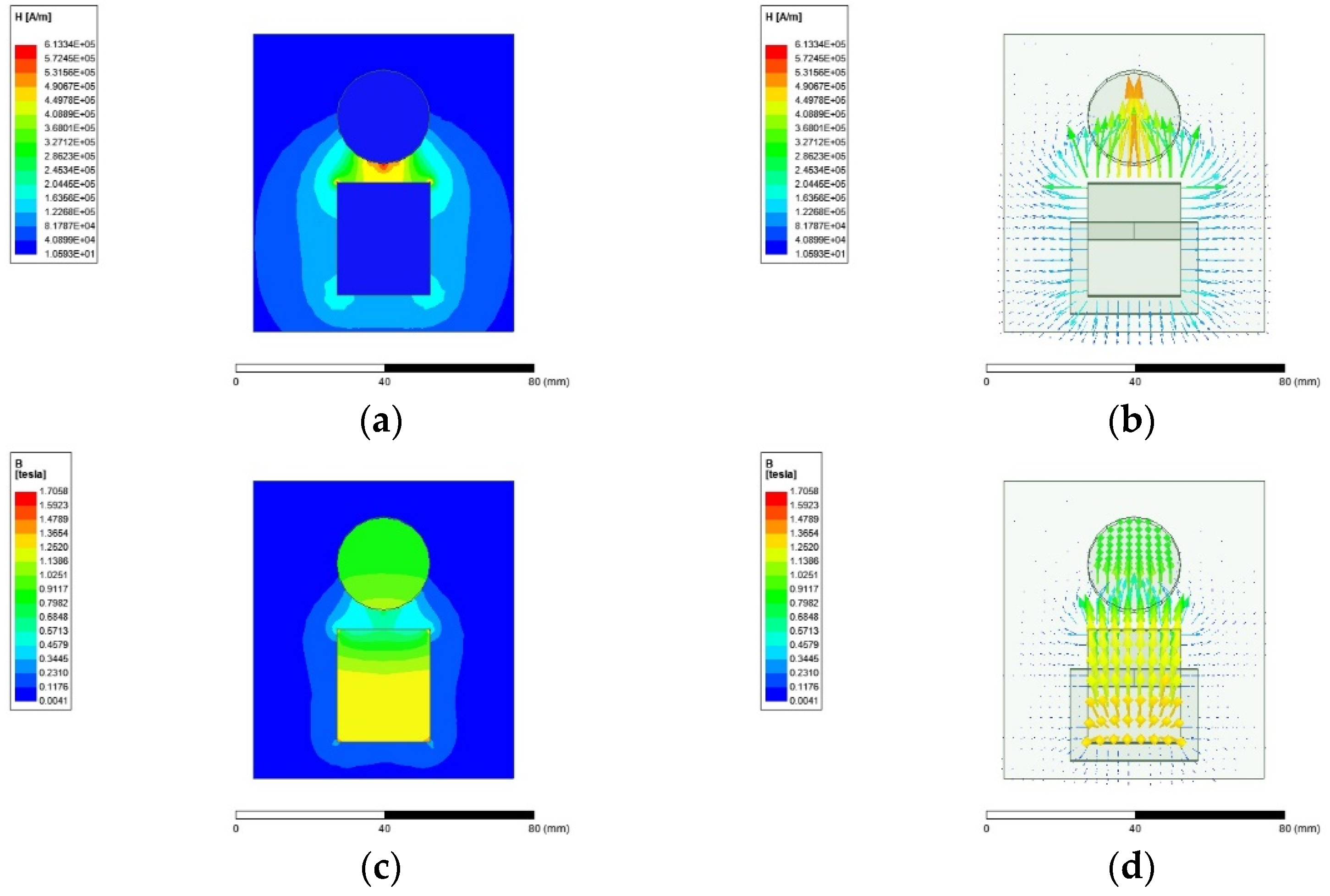
In typical fixed–value state investigation experiments, the purpose of the experiment is to investigate the real–time state of the electromagnetic field at the time of the effective adsorption of the model. Experimental conditions: the radius of the reinforcement bar is 12.5 mm; the gap distance is 5 cm; the number of turns of the coil is 195; the rotation angle is 0°; and the input current is 10 A. After the experiment, according to the experimental results, the intensity distribution and motion vector of the magnetic field strength and magnetic flux density of different inspection surfaces are generated as illustrated in Figure 18 and Figure 19.

The experimental model is equivalent to an annular closed magnetic core with an air gap. The relative permeability of the iron core of the electromagnetic unit and the reinforcement bars in the borehole wall is very large. Therefore, the magnetic field strength is mainly concentrated in the air gap, and the storage capacity inside the iron core and the reinforcement bars is extremely small, as shown in Figure 18a. The direction of magnetic flux movement is circular. The magnetic field strength in the vertical direction at the air gap is the greatest, and the edge magnetic flux at the inner and outer corners of the end of the unit has a strong magnetic field strength, as shown in Figure 18b. The magnetic flux is the same everywhere in the electromagnetic circuit, and the magnetic flux density is proportional to the area of the magnetic circuit channel. At the yoke of the iron core, the magnetic flux is relatively concentrated, and the channel area is smallest. Thus, the magnetic flux density here is the largest. At the air gap, due to the divergence of the edge magnetic flux, the magnetic flux density here is the smallest, as exhibited in Figure 18c. The vector direction of the magnetic flux density is consistent with the magnetic field strength, but the intensity distribution is the opposite, as shown in Figure 18d.

The electromagnetic intensity and magnetic flux density diagram of the longitudinal investigation surface of the experiment are shown in Figure 19. It can be observed that the magnetic field intensity distribution and motion vector direction of the magnetic flux in the longitudinal direction of the model are consistent with the experimental results of the transverse inspection surface. In the meantime, the value of the magnetic field strength in the midline of the width of the side of the unit reaches the maximum. Subsequently, it gradually decreases to both sides, and the direction of the magnetic flux vector also shows a clear trend of movement from both sides to the center. The electromagnetic intensity is mainly concentrated in the normal direction of the end of the unit, and it is negligible in the tangent direction.

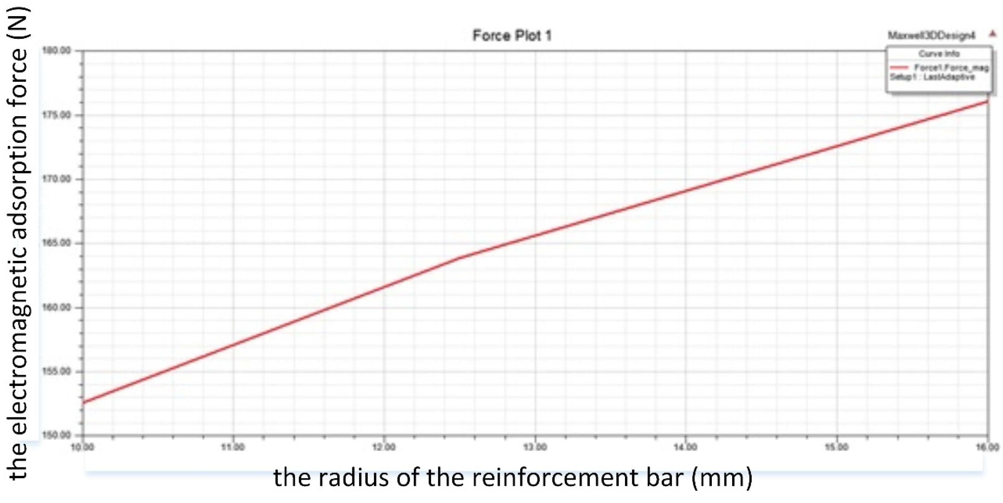
The purpose of the investigation experiment of the law of interval variables is to investigate the law of change of the electromagnetic adsorption force generated by the model within the limit range of different variables. The sub–experimental conditions are as follows: 1. the radius of the reinforcement bar is from 0 to 16 mm; 2. the rotation angle is from 0° to 30°; and 3. the input current is from 0 to 10 A. In the sub–experiment, in addition to the experimental variables, the general values of other experimental parameters are selected. After the experiment, based on the experimental results, the numerical corresponding curve is generated, as shown in Figure 20, Figure 21 and Figure 22. Among them, increasing the radius of the reinforcement bar and increasing the input current are conducive to increasing the magnetic flux in the electromagnetic circuit and increasing the electromagnetic adsorption force. Increasing the rotation angle is equivalent to reducing the effective adsorption area of the electromagnetic unit and the reinforcement bar in the lining, so that the electromagnetic adsorption force is reduced. In the corresponding curve of the value, the value of the electromagnetic adsorption force changes linearly within the expected range with the change of the experimental variable, and it is concluded that the simulation experiment results are consistent with the calculation results of the formula.

6. Efficiency Analysis of Coupling Adsorption Mechanism

The theoretical basis and mechanism of electromagnetic adsorption are distinct from those of negative pressure adsorption. The power loss generated in the adsorption production process is different. For the study of the law of the change of system power with the output adsorption force in the coupled adsorption mechanism, the power calculation results of the two adsorption methods should be summarized, and the overall power of the electromagnetic adsorption device and the negative pressure adsorption device under the same adsorption force requirements should be compared and analyzed.

(1)

Calculation of loss and power of centrifugal fan

The loss of air flow in the negative pressure adsorption device mainly occurs in the centrifugal fan stage, which specifically includes leakage loss, flow loss, and mechanical loss. Among them, leakage loss reduces system flow, flow loss reduces fan static pressure, and mechanical loss increases power consumption. Among the above three losses, the first two consume system power indirectly by reducing the operating efficiency of the fan, while the latter rely on the system to directly increase the output power to offset the loss [25,26,27,28].

Normally, leakage loss refers to the loss of gas flow leaked by the gap between the inner wall baffle of the negative pressure chamber and the front cover of the centrifugal fan. Under actual working conditions (P_t = 2002 Pa), the leakage loss Δq_v of the centrifugal fan is as below:

$$\Delta q_v=2\pi D_{1}a\delta \sqrt{\frac{p_t}{3\rho }}$$

(13)

Among which:

Δq_v—The loss of gas flow (m³);

δ—Clearance distance, δ = 2 mm;

a—Clearance edge shrinkage coefficient, a = 07.

Substitute the data and calculate, Δq_v = 0.0311 m³. Then, the theoretical flow rate of the centrifugal fan is

$$q_l=q_v+\Delta q_v$$

(14)

Substituting the working conditions gas flow rate q_v = 0.5548 m³ calculated by Equation (4) into Equation (14), q_l = 0.5859 m³ can be obtained.

Mainly, the flow loss includes the axial and radial conversion pressure loss caused by the change in the direction of fluid movement, the pressure loss of the blade channel generated by the air flow between the adjacent blades of the impeller, and the outlet diffuser pressure loss caused by the deceleration of the fluid caused by the increase in the fan outlet fluid channel [29,30,31,32].

The air flow axis and radial conversion pressure loss Δp₁ is as below:

$$\Delta p_1={\zeta }_1\rho \frac{v_1^2}{2}$$

(15)

Among which:

v₁—Absolute velocity of airflow at blade inlet (m/s);

ζ₁—Loss coefficient, ζ₁ = 0.15.

The absolute velocity of airflow at blade inlet v₁ is equal to the normal velocity of the vector diameter v_1n:

$$v_1=v_{1n}=\frac{q_l}{\pi D_1{b}_1}$$

(16)

Substitute the data and calculate, v₁ = 20.7223 m/s, Δp₁ = 38.8048 Pa.

The pressure loss of the air flow blade channel, Δp₂, is

$$\Delta p_2={\zeta }_2\rho \frac{v_{1r}^2}{2}$$

(17)

Among which:

v_1r—Relative velocity of airflow at blade inlet (m/s);

ζ₂—Loss coefficient, ζ₂ = 0.15.

Based on the fluid inlet velocity triangle, the relative velocity of airflow at blade inlet v_1r is

$$v_{1r}=\frac{v_1}{\sin ({\beta }_{1A})}$$

(18)

Substitute the data and calculate, v_1r = 36.1283 m/s, Δp₂ = 117.9624 Pa.

The diffuser pressure loss at the air fluid outlet Δp₃ is

$$\Delta p_3={\zeta }_3\rho \frac{v_2^{,}{}^2}{2}$$

(19)

Among which:

v₂—Absolute velocity of airflow at blade outlet (m/s):

ζ₃—Loss coefficient, ζ₃ = 0.15.

Substitute the data and calculate, v₂ = 36.2760 m/s, Δp₃ = 118.9287 Pa.

Under actual working conditions, the total flow loss of the centrifugal fan is

$$\Delta p_h=\Delta p_1+\Delta p_2+\Delta p_3$$

(20)

Substituting the calculation result of (15), (17) and (19) into Equation (20), Δp_h = 275.6995 Pa can be obtained.

Mechanical loss, also known as roulette wheel friction loss, is characterized by a certain flow and pressure loss. However, it only causes power loss, does not reduce the full pressure of the fan, and has no effect on the theoretical flow rate. Under actual working conditions, the mechanical loss of the centrifugal fan is

$$\Delta q_r=\rho D_2^2{v}_{2e}^3\frac{B_d}{{10}^6}$$

(21)

Among which:

v_2e—Entrainment velocity of blade outlet flow (m/s);

B_d—Strouhal coefficient, B_d = 0.81.

Substitute the data and calculate, v₂ = 62.8319 m/s, Δq_r = 3.4679 × 10⁻⁴. Through the calculation results, it is found that the mechanical loss value of the centrifugal fan is extremely small under the negative pressure condition of the system with the largest system demand.

In the centrifugal fan stage, after all the itemized analysis of possible energy loss and based on the centrifugal fan power calculation formula, the effective power of the centrifugal fan is as follows:

$$P_e=P_t{q}_v$$

(22)

Substitute the data and calculate, P_e = 1110.7 W; the internal power of the centrifugal fan is

$$P_{in}=\left(P_t+\Delta P_h\right)(q_v+\Delta q_v)+\Delta P_r$$

(23)

Substitute the data and calculate, P_in = 1334.5 W. When the centrifugal fan is directly connected to the drive motor, the mechanical efficiency of the fan is ƞ_m = 1. Numerically, the internal power of the centrifugal fan is equal to the shaft power—that is, the input power of the centrifugal fan [33,34,35,36].

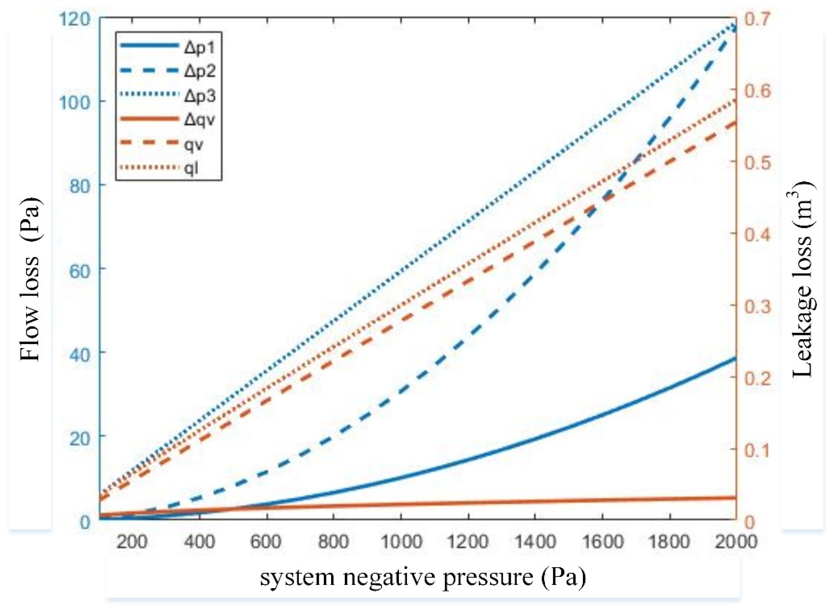
The corresponding curve of the negative pressure and flow loss and leakage loss of the centrifugal fan system is illustrated in Figure 23. The impact of fan mechanical loss on system power is too small to be excluded in the figure. According to the figure, in the pressure flow loss part, the loss coefficients of the three losses are the same. The degree of loss is principally dominated by the itemized velocity of the fluid entering the inspection channel, as well as the leakage loss and the inlet angle. Among them, the outlet diffuser pressure loss directly depends on the negative pressure of the system; the shaft, radial conversion loss, and blade channel loss are indirectly determined by the negative pressure of the system; and the total amount of pressure loss increases with the increase in the negative pressure of the system. In the flow leakage loss process, as the negative pressure of the system increases, the fluid leakage flow rate increases little by little, but it is always maintained at a low level without causing much impact on the system’s power. The difference between the theoretical flow rate of the fan and the actual flow rate is proportional to the leakage flow rate. To sum up, it is verified that the negative pressure of the system is the major factor that determines the total power loss of the centrifugal fan. Under the condition of high negative pressure demand, the negative pressure adsorption system should put out more compensation power. The experimental numerical calculation results can be found in Appendix A 

Table A3. Centrifugal fan loss and power table.

System Negative Pressure Pt (Pa)	Flow Loss (Pa)			Leakage Loss Δqv (m3)	Mechanical Loss Δqr (W)	Effective Power Pe (W)	Input Power Pin (W)
	Δp1	Δp2	Δp3
100	0.1358	0.4127	5.9404	0.0069	1.73 × 10−5	2.7715	3.6903
200	0.4812	1.4627	11.8807	0.0098	3.46 × 10−5	11.0858	13.9507
300	1.0238	3.1119	17.8211	0.0120	5.19 × 10−5	24.9431	30.6387
400	1.7590	5.3466	23.7614	0.0139	6.92 × 10−5	44.3434	53.7455
500	2.6842	8.1589	29.7018	0.0155	8.66 × 10−5	69.2865	83.2931
600	3.7977	11.5436	35.6422	0.0170	1.03 × 10−4	99.7725	119.3166
700	5.0983	15.4967	41.5825	0.0184	1.21 × 10−4	135.8015	161.8585
800	6.5848	20.0152	47.5229	0.0196	1.38 × 10−4	177.3734	210.9656
900	8.2565	25.0966	53.4632	0.0208	1.55 × 10−4	224.4882	266.6879
1000	10.1128	30.7389	59.4036	0.0219	1.73 × 10−4	277.1459	329.0771
1100	12.1531	36.9405	65.3439	0.0230	1.90 × 10−4	335.3466	398.1865
1200	14.3768	43.6999	71.2843	0.0240	2.07 × 10−4	399.0902	474.0706
1300	16.7837	51.0158	77.2247	0.0250	2.25 × 10−4	468.3766	556.7845
1400	19.3732	58.8871	83.1650	0.0260	2.42 × 10−4	543.2061	646.3844
1500	22.1452	67.3127	89.1054	0.0269	2.59 × 10−4	623.5784	742.9265
1600	25.0992	76.2918	95.0457	0.0278	2.77 × 10−4	709.4936	846.4680
1700	28.2351	85.8236	100.9861	0.0286	2.94 × 10−4	800.9518	957.0659
1800	31.5525	95.9073	106.9265	0.0294	3.11 × 10−4	897.9529	1074.7781
1900	35.0513	106.5422	112.8668	0.0302	3.29 × 10−4	1000.4969	1199.6621
2000	38.7312	117.7277	118.8072	0.0310	3.46 × 10−4	1108.5838	1331.7762

.

(2)

Comparative analysis of adsorption force and power

The corresponding curves of the various power parameters in the process of generating electromagnetic adsorption force by the single electromagnetic unit in the electromagnetic array are displayed in Figure 24. From Figure 24a, the electromagnetic adsorption force of the unit increases with the increase in the magnetic flux of the channel. It is verified that under the premise of certain structural parameters, material parameters, and the number of turns of the wire, the electromagnetic adsorption system enhances the electromagnetic adsorption force of the unit by increasing the input current and then enhancing the magnetic flux in the magnetic circuit channel. In Figure 24b, the electromagnetic power of the unit increases with the increase in the input current, and the standard curve slope shows an increasing trend, implying that the input current is the principal factor determining the power of the electromagnetic unit. Furthermore, in the initial stage of increasing the input current of the unit, the electromagnetic adsorption force is slightly increased; the loss of electromagnetic power is relatively small. In the stage of increasing the input current of the unit from 1/3 node to the numerical boundary, the increase in electromagnetic adsorption force and electromagnetic power is faster, indicating that the power loss of the electromagnetic unit is small when it starts. The experimental numerical calculation results can be found in Appendix A 

Table A4. Electromagnetic array current and power table.

Electromagnetic Adsorption Force F (N)	2 Sets of Electromagnetic Units			4 Sets of Electromagnetic Units			Array Power P (W)
	Input Current I1 (A)	Magnetic Flux Φ1 (Wb)	Unit Power P1 (W)	Input Current I2 (A)	Magnetic Flux Φ2 (Wb)	Unit Power P2 (W)
10	1.7456	1.34 × 10−6	1.4495	1.2343	9.51 × 10−7	0.7247	2.8990
20	2.4687	1.90 × 10−6	2.8990	1.7456	1.34 × 10−6	1.4495	5.7980
30	3.0235	2.33 × 10−6	4.3485	2.1379	1.64 × 10−6	2.1742	8.6969
40	3.4912	2.69 × 10−6	5.7980	2.4687	1.90 × 10−6	2.8990	11.5959
50	3.9033	3.01 × 10−6	7.2474	2.7601	2.12 × 10−6	3.6237	14.4949
60	4.2759	3.29 × 10−6	8.6969	3.0235	2.33 × 10−6	4.3485	17.3939
70	4.6185	3.56 × 10−6	10.1464	3.2657	2.51 × 10−6	5.0732	20.2928
80	4.9373	3.81 × 10−6	11.5959	3.4912	2.69 × 10−6	5.7980	23.1918
90	5.2368	4.03 × 10−6	13.0454	3.7030	2.85 × 10−6	6.5227	26.0908
100	5.5201	4.25 × 10−6	14.4949	3.9033	3.01 × 10−6	7.2474	28.9898
110	5.7896	4.46 × 10−6	15.9444	4.0938	3.15 × 10−6	7.9722	31.8888
120	6.0470	4.66 × 10−6	17.3939	4.2759	3.29 × 10−6	8.6969	34.7877
130	6.2939	4.85 × 10−6	18.8434	4.4505	3.43 × 10−6	9.4217	37.6867
140	6.5315	5.03 × 10−6	20.2928	4.6185	3.56 × 10−6	10.1464	40.5857
150	6.7607	5.21 × 10−6	21.7423	4.7806	3.68 × 10−6	10.8712	43.4847
160	6.9825	5.3 × 10−6	23.1918	4.9373	3.80 × 10−6	11.5959	46.3836
170	7.1974	5.55 × 10−6	24.6413	5.0893	3.92 × 10−6	12.3207	49.2826
180	7.4060	5.71 × 10−6	26.0908	5.2368	4.03 × 10−6	13.0454	52.1816
190	7.6090	5.86 × 10−6	27.5403	5.3803	4.14 × 10−6	13.7701	55.0806
200	7.8066	6.01 × 10−6	28.9898	5.5201	4.25 × 10−6	14.4949	57.9796
210	7.9994	6.16 × 10−6	30.4393	5.6564	4.36 × 10−6	15.2196	60.8785
220	8.1877	6.31 × 10−6	31.8888	5.7896	4.46 × 10−6	15.9444	63.7775
230	8.3717	6.45 × 10−6	33.3382	5.9197	4.56 × 10−6	16.6691	66.6765
240	8.5517	6.59 × 10−6	34.7877	6.0470	4.66 × 10−6	17.3939	69.5755
250	8.7281	6.73 × 10−6	36.2372	6.1717	4.75 × 10−6	18.1186	72.4744
260	8.9009	6.86 × 10−6	37.6867	6.2939	4.85 × 10−6	18.8434	75.3734
270	9.0705	6.99 × 10−6	39.1362	6.4138	4.94 × 10−6	19.5681	78.2724
280	9.2369	7.12 × 10−6	40.5857	6.5315	5.03 × 10−6	20.2928	81.1714
290	9.4004	7.24 × 10−6	42.0352	6.6471	5.12 × 10−6	21.0176	84.0704
300	9.5611	7.37 × 10−6	43.4847	6.7607	5.21 × 10−6	21.7423	86.9693
310	9.7192	7.49 × 10−6	44.9342	6.8725	5.29 × 10−6	22.4671	89.8683
320	9.8747	7.61 × 10−6	46.3836	6.9825	5.38 × 10−6	23.1918	92.7673
330	10.0278	7.73 × 10−6	47.8331	7.0907	5.46 × 10−6	23.9166	95.6663
340	10.1786	7.84 × 10−6	49.2826	7.1974	5.55 × 10−6	24.6413	98.5653
350	10.3272	7.96 × 10−6	50.7321	7.3024	5.63 × 10−6	25.3661	101.4642
360	10.4737	8.07 × 10−6	52.1816	7.4060	5.71 × 10−6	26.0908	104.3632
370	10.6182	8.18 × 10−6	53.6311	7.5082	5.78 × 10−6	26.8155	107.2622
380	10.7607	8.29 × 10−6	55.0806	7.6090	5.86 × 10−6	27.5403	110.1612
390	10.9014	8.40 × 10−6	56.5301	7.7084	5.94 × 10−6	28.2650	113.0601
400	11.0402	8.51 × 10−6	57.9796	7.8066	6.01 × 10−6	28.9898	115.9591

.

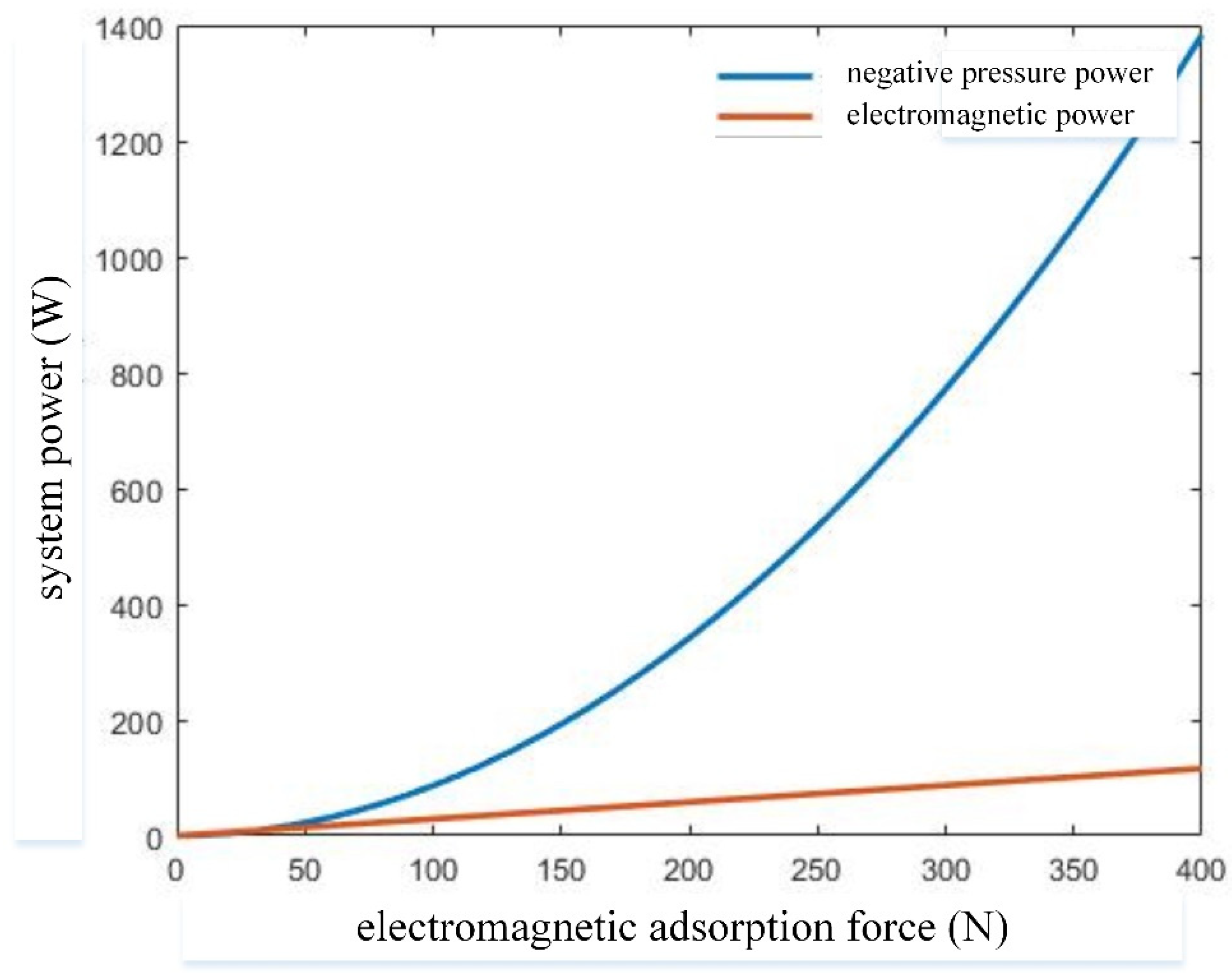
The power comparison curve of the electromagnetic adsorption device and the negative pressure adsorption device corresponding to the adsorption force output value in the coupled adsorption system is shown in Figure 25. Based on the observation of the curve in the figure, under the premise of outputting the same adsorption force, the power consumption of the negative pressure adsorption system is much larger than that of the electromagnetic adsorption system. Furthermore, within the range of the adsorption force inspection interval, the power increment of the negative pressure adsorption system is much greater than that of the electromagnetic adsorption system. Through numerical comparison and analysis, it can be inferred that to maintain the stable operation of the wall–climbing robot on the vertical shaft lining, the negative pressure adsorption method is bound to consume several times the energy and power of the electromagnetic adsorption method, and the adsorption efficiency of electromagnetic adsorption is significantly higher than that of negative pressure adsorption.

7. Conclusions

Based on high–performance simulation software, the electromagnetic and negative pressure coupling adsorption process was experimentally studied. The experimental results were consistent with the expected requirements. The experimental data are expected to provide a reference for researchers in the same field. The main research conclusions are as follows:

(1)

The main velocity and direction of movement of the air flow in the fluid channel depend on the pressure difference between the inside and the outside of the sealing device. The main velocity and direction of movement of the air flow inside the negative pressure chamber are determined by the centrifugal fan speed. Under the conditions of channel height h > 1.72 mm and fluid flow rate < 50 m³/s, it is difficult for the negative pressure adsorption system to have the basic conditions for forming a stable negative pressure.

(2)

The fluid velocity of the air flow in the radial direction of the fan is separated under the action of the fan blade. The value of each speed component shows a positive linear relationship with the fan speed, increasing with the increase in fan speed. Under different speed conditions, the circulation coefficient and flow efficiency of the fan converge to the same value, which are 0.8654 and 0.9118, respectively.

(3)

In the electromagnetic circuit, the magnetic field strength in the air gap is the highest, and the magnetic flux density of the yoke of the unit iron core is the largest. Increasing the radius of the reinforcement bar and the input current is conducive to increasing the electromagnetic adsorption force and the rotation angle, resulting in a decrease in the electromagnetic adsorption force. The input current of the unit is the principal factor that dominates the electromagnetic adsorption force and system power.

(4)

The adsorption efficiency of electromagnetic adsorption is significantly better than that of negative pressure adsorption. The power loss in the start–up phase of the negative pressure adsorption system is serious; consequently, the repeated start and stop of the negative pressure device should be avoided as much as possible in the power distribution of the coupled adsorption system. Meanwhile, the power loss in the start–up phase of the electromagnetic adsorption system is relatively slight; therefore, the repeated start and stop of the electromagnetic unit will not increase the overall power consumption of the coupled adsorption system.

In this paper, the research results of the investigation into the speed separation phenomenon of air flow during the movement of centrifugal fans and the power changes of electromagnetic and negative pressure systems during start–up and speed–up are of innovative significance. In the future, the author will continue to engage in research on wall–climbing robots in the field of coal mine safety, with the development of automatic control systems for wall–climbing robots as the main direction. Moreover, under the premise of project funds permitting, prototypes shall be made.