Article

A Methodology for Consolidation Effects of Inventory Management with Serially Dependent Random Demand

1
School of Industrial Engineering, Pontificia Universidad Católica de Valparaíso, Valparaíso 2362807, Chile
2
Eating Behavior Research Center, School of Nutrition and Dietetics, Faculty of Pharmacy, Universidad de Valparaíso, Valparaíso 2360102, Chile
3
Center of Micro-Bioinnovation, Faculty of Pharmacy, Universidad de Valparaíso, Valparaíso 2360102, Chile
4
COPPEAD, Universidade Federal de Rio de Janeiro, Rio de Janeiro 21941-918, Brazil
5
Centro de Estudios e Investigaciones Estadísticas, Escuela Superior Politécnica del Litoral, Guayaquil 090902, Ecuador
*
Author to whom correspondence should be addressed.
Processes 2023, 11(7), 2008; https://doi.org/10.3390/pr11072008
Submission received: 17 May 2023 / Revised: 20 June 2023 / Accepted: 22 June 2023 / Published: 5 July 2023

Abstract

:
Most studies of inventory consolidation effects assume time-independent random demand. In this article, we consider time-dependence by incorporating an autoregressive moving average structure to model the demand for products. With this modeling approach, we analyze the effect of consolidation on inventory costs compared to a system without consolidation. We formulate an inventory setting based on continuous-review using allocation rules for regular transshipment and centralization, which establishes temporal structures of demand. Numerical simulations demonstrate that, under time-dependence, the demand conditional variance, based on past data, is less than the marginal variance. This finding favors dedicated locations for inventory replenishment. Additionally, temporal structures reduce the costs of maintaining safety stocks through regular transshipments when such temporal patterns exist. The obtained results are illustrated with an example using real-world data. Our investigation provides information for managing supply chains in the presence of time-patterned demands that can be of interest to decision-makers in the supply chain.

1. Introduction

This section provides the introduction, state-of-the-art, contributions, objectives, and plan of the sections used in this article.

1.1. Introduction and Bibliographical Review

In the supply chain, items are typically transferred from producers to distribution centers and then sold to retailers [1]. To create an efficient network, companies aim to minimize costs while maintaining a high level of service [2]. This can be achieved by making decisions regarding the facility location, number of distribution centers serving demand, and supply frequency [3].
One common approach is to set up a supply chain where each dedicated facility serves the demand per unit of time (DPUT), resulting in an independent system (IS) [4,5]. Thus, we define an IS as a framework where each decentralized location is served exclusively by a single centralized location. However, when demand for each dedicated facility in an IS exhibits high variability, costs associated with maintaining service levels, such as holding costs, tend to increase [6]. In such cases, inventory pooling can be implemented through centralized or regular supply using transshipment.
A centralized inventory is given when all decentralized locations are served by a single centralized location, while a regular transshipment (RT) occurs when all decentralized locations are served by all centralized locations. This approach can significantly reduce demand variability at individual points and often lead to cost savings compared to an IS [6,7,8].
The study conducted in [7] examined inventory pooling defined as a setting in supply chain to group goods minimizing the system’s cost in multiple locations. In [7], it was also investigated the cost reductions associated with inventory pooling and its relationship with demand variability assuming independent and identically distributed (IID) demand. The research [7] concluded that centralization is necessary for improving system operation when demand varies significantly across different areas. In a study given in [9], centralized and decentralized supply chains with uncertain supply were compared. The centralized network leveraged risk-pooling effects by combining demand variation from numerous sites, resulting in lower inventory costs and expected total costs (TC). In [10], the authors extended the concept of consolidated safety stock ( SS c ) to multiple storage points, while in [11], it was conducted a similar analysis for consolidated cycle stock ( CS c ). Recent techniques have explored cost reduction by identifying potential consolidation facilities that combine shipments with improved service levels [12].
The selection of appropriate demand allocation rules is crucial for considering the consolidation effect [6]. The Tyagi-Das (TD) rule is one of such approaches, where an equal demand is distributed to decentralized sites from a specific centralized location [5]. When using the TD rule and assuming IID DPUTs over time, the maximum consolidation impact is determined by the lead time (LT) between sites [6]. Consolidation is most effective when the consolidated TC ( TC c ) and inventory decrease. If the mean and standard deviation (SD) of the LT are the same at both centralized locations, the demand provided to decentralized sites should also be the same. Thus, when inventories are consolidated in a single place, the maximum consolidation impact is achieved by employing distinct means/SDs for LT and DPUT [6]. Another allocation approach is the Ballou-Burnetas (BB) rule, where a portion of the demand is met by a main location and the remaining demand by other secondary locations [4]. For IID DPUTs over time, RT is a suitable choice when DPUTs in each centralized site are directly correlated. This approach balances small/large mean/SD for LT and DPUT at various centralized locations and is particularly effective when the holding cost (HC) is relatively small  [6].
Inventory pooling primarily reduces costs by decreasing the inventory level required to meet a given service level. Nonetheless, inventory centralization (IC) does not only impact HC [6]. In general, the  TC c and IS TC ( TC i ) in an inventory pooling system consist of four costs associated with SS and average inventory, including the ordering cost (OC), storage cost, and distribution cost (DC) over a given period [6,13]. For the TC c , the four cost components are: (CC1) HC multiplied by SS c ; (CC2) HC multiplied by CS c ; (CC3) consolidated DC ( DC c ); and (CC4) consolidated OC ( OC c ) [6]; also refer to Section 2.3. The total SS under inventory pooling is crucially influenced by the randomness of DPUT and the LT period [13].
To reduce the TC c , previous studies given in [6,11] used mathematical treatments of the consolidation effect by assuming random DPUT and the following: (a) all locations utilize a SS before and after consolidation, considering the uncertainty of LT demand (LTD); (b) all locations employ the same safety factor for the desired service level; (c) each location adopts a continuous-review model for lot size and reorder point in inventory control; (d) the total average demand of the system remains constant after consolidation; and (e) DPUT and LT are independent. Recent studies conducted in [14,15] extended these approaches by considering an asymmetric distribution for the DPUT and various degrees of kurtosis. These studies demonstrated that the TC c decreases under specific conditions, including the level of correlation among DPUTs at different locations, mean/SD of DPUTs and LT, safety factor for LTD, and costs associated with holding, ordering, and distribution [6].

1.2. Contribution, Objectives, and Organization of the Article

The main findings from prior research are: (a) small TC c values generated by centralized locations are linked to indirect correlations between the DPUTs and high values of DPUT SDs; (b) positive correlations between DPUTs and small values for DPUT SD are associated with the use of an IS supply; and (c) distinct SDs for the LT are managed in a better way by an RT due to the combination and balancing of the DPUTs that an RT serves. In [14,16], the authors confirmed the previous conclusions for non-Gaussian distributions. However, these works employed a continuous-review model with IID DPUT. Recent research has considered the dependence on DPUT [17]. Copulas methods have been the primary focus for modeling the joint DPUT distribution [11,18,19]. Nevertheless, it should be noted that DPUTs often exhibit time-dependence, as highlighted in [20]. In this dependence framework, an autoregressive moving average (ARMA) model can adequately describe time-dependent DPUT [21]. In this context, in [22], it was warned of a gap in the literature on inventory models between those that incorporate temporal dependence and those that do not. Also, the consideration of ARMA models makes it possible to better capture the behavior of customer demand in cases of temporal dependency. This dependency improves the accuracy of the forecasts. Thus, inventory management, which can be considered in customer relationship management (CRM) models to improve customer demand, enables us to plan seasonal marketing with product delivery on time.
One of the few works on consolidation effects in inventories under time-dependent DPUTs is attributed to [23]. These authors found the optimal SS by assuming homogeneity in the DPUT variability and considering the temporal correlation. In [24], optimal policies and approximations were proposed for inventories with temporally correlated demand in a similar setting, although not on the consolidation impact.
Given that ARMA models are commonly used to model time-dependent demand [25], its characteristic and how they can be incorporated into different allocation rules are of interest. One unique characteristic of the ARMA models is that the variance of the random variable (RV) of interest in a time-dependent framework is conditional on past data, and it is less than the marginal variance in an independent framework. Since decreasing demand variability results in cost savings under inventory pooling, this suggests that the precision of the inventory model increases when analyzing such demand time series, leading to a decrease in TC c through allocation rules. However, to the best of our knowledge, there is a gap in the literature because no studies have analyzed how the temporal dependence of demand affects the TC c of a pooled inventory for different allocation rules.
To address this gap, our investigation designs a procedure to analyze how the temporal dependence described by an ARMA model impacts the TC c of a pooled inventory for distinct allocation rules. Specifically, our study includes: (i) comparing the TC between a system with inventory pooling and IS under time-dependence; and (ii) analyzing changes in metrics of inventory TC, under the previously assumed scenarios but adding temporality.
The rest of the paper is as follows. Section 2 introduces our approach upon two pillars: (a) modeling assuming an IID DPUT and modeling DPUT based on an ARMA model for temporal dependence; and (b) the consolidation effects of inventory. In Section 3, we perform simulations to analyze how time-dependence affects TC c of inventories for distinct allocation rules. Section 4 analyzes an illustrative example with real data and guidelines on the theme are established. Section 5 discusses our investigation and states concluding remarks, limitations, and proposals to continue investigating the theme of the present study.

2. Proposed Methodology

Given the presence of correlated demand over time, we propose using the following methodology to consolidate inventories. To carry out our study, we have followed the approach given in [6] which assumed IID demands. However, to derive a consolidation effect on time-dependent demand, we relax the IID assumption by assuming an ARMA model for DPUT. Next, this section states the new approach introduced in the present investigation.

2.1. Modeling DPUT without Temporal Dependence

Suppose that an IID RV Z models the randomness of the DPUT with a normal distribution. Then, Z has a probability density function (PDF) given by
f Z ( z ) = 1 2 π σ Z 2 exp ( z μ Z ) 2 2 σ Z 2 , z R , μ Z R , σ Z > 0 ,
with μ Z and σ Z 2 denoting the statistical parameters related to the marginal mean and variance of Z, respectively. In the usual regression model, μ Z can be described by the values of r explanatory variables (also called independent variables or covariates) summarized in the ( r + 1 ) × 1 vector of values x = ( 1 , x 1 , , x r ) by means of
μ Z = E ( Z ) = x β ,
where β = ( β 0 , β 1 , , β r ) is the coefficient vector related to each element of x .
Let Z 1 and Z 2 denote IID RVs which have a cumulative distribution function (CDF) F Z 1 , Z 2 . Hence, we get a relation given by
C ( c , d ; ϱ ) = F Z 1 , Z 2 ( F Z 1 1 ( c ) , F Z 2 1 ( d ) ) , c , d [ 0 , 1 ] ,
where
ϱ = ϱ Z 1 , Z 2 = Cov ( Z 1 , Z 2 ) σ Z 1 2 σ Z 2 2 ,
with ϱ denoting a dependence parameter between Z 1 , Z 2 , and σ Z 1 2 = V ( Z 1 ) and σ Z 2 2 = V ( Z 2 ) . Hence, from the formula stated in (2) and in [16], we reach that the PDF related to C ( u , v , ϱ ) is established as
c ( F Z 2 ( z 2 ) , F Z 1 ( z 1 ) , ϱ Z 1 , Z 2 ) = 2 C F Z 2 F Z 1 ,
where denotes the corresponding partial derivatives. For more details about the use of copulas to model the correlated DPUTs in consolidated effects, see [11].

2.2. Modeling DPUT with Temporal Dependence

To describe the DPUT when it is time-dependent, we can employ an RV Z t measured at time t with t { 1 , , N } . For this purpose, we may consider the conditional normal distribution of Z t depending on a past data set H t { x 1 , , x t , z 1 , , z t 1 } by an ARMA model of p (autoregressive) and q (moving average) orders, that is, ARMA( p , q ), with  x 1 , , x t and z 1 , , z t 1 being the observed values of x and Z, respectively, at the corresponding instants of time. Through this model, the mean of Z t can be formulated as
μ Z t = E ( Z t ) = x t β + l = 1 p ϕ l ( z t l x t l β ) + m = 1 q ϑ m ( z t m μ t m ) ,
with ϕ l , ϑ m being the l-th and m-th elements of an ARMA structure, respectively, of  p , q orders, and  β is defined as in (1), but now related to r covariates depending over time, that is, x t = ( 1 , x 1 t , , x r t ) .
If we define a martingale residual as U t = Z t μ Z t for the model error and state V t = Z t x t β , from (4), we can take the expression given by
V t = h = 1 p ϕ h v t h + j = 1 q ϑ j u t j + U t .
Now, if we consider the lag operators presented as
Φ ( M ) = 1 ϕ 1 L ( 1 ) ϕ p L ( p ) ,
ϑ ( M ) = 1 + ϑ 1 M ( 1 ) + + ϑ q M ( q ) ,
then, we may rewrite the model defined in (5) as
V t = ϑ ( M ) Φ ( M ) U t = Ψ ( M ) U t ,
with
Ψ ( M ) = ϑ ( M ) Φ ( M ) = 1 + ψ 1 M ( 1 ) + ψ 2 M ( 2 ) + ,
and Φ ( M ) being an invertible function. In [26], it was proved that, for the RV Z, its marginal mean and variance are stated as
μ Z t = E ( Z t ) = E ( x t β + V t ) = E ( x t β ) + E ( V t ) = x t β , t , σ Z t 2 = V ( Z t ) = V ( V t ) = E ( V t 2 ) = Ψ ( 2 ) ( M ) V ( Z t | H t ) , t ,
where Ψ ( 2 ) ( M ) = 1 + ψ 1 2 L ( 1 ) + ψ 2 2 L ( 2 ) + , for stationary and invertible time series.
Remark 1. 
Note that Ψ ( 2 ) ( M ) 1 . Thus, the variance conditional on past data is less than the marginal variance, that is, when no temporal disposition of the data is considered. In the modeling, consider the assumption that σ Z t 2 is invariant over time.
Now, if we define an RV T as the random LT, with T being independent of Z t , then the random sum S of Z t for an item under inventory until reaching LT is expressed as S = t = 1 T Z t . We denote the PDF of S as f S , which is defined on [ 0 , ] (non-negative support), and its CDF is given by F S ( r ) = 0 r f S ( x ) d x , with its quantile function being stated as F S 1 ( x ) , for  x [ 0 , 1 ] . The conditional mean and variance of S on past data, H t namely, are defined, respectively, as
μ S t = E ( S | H t ) = μ T E ( Z t | H t ) = μ T μ Z t ,
σ S t 2 = V ( S | H t ) = σ T 2 E 2 ( Z t | H t ) + μ T V ( Z t | H t ) = σ T 2 μ Z t 2 + μ T σ Z t 2 ,
where μ T = E ( T ) and σ T 2 = V ( T ) . Note that for IID DPUTs, the expressions given in (10) and (11) reduce to
μ S = E ( S ) = E ( T ) E ( Y ) = μ T μ Y , σ S 2 = V ( S ) = V ( T ) E 2 ( Y ) + E ( T ) V ( Y ) = σ T 2 μ Y 2 + μ T σ Y 2 .
The data generated from a bivariate ARMA model conditional on past data are presented in [27]. Generalized volatile multivariate time series models by using the Cholesky decomposition were presented in [28]. With this generalization, it is possible to parameterize the variance-covariance matrix of a bivariate ARMA model for Z 1 t = μ Z 1 t + U 1 t and Z 2 t = μ Z 2 t + U 2 t , which can be related by using the regression model given by
U 2 t = β u 1 t + ε 2 t ,
where β is a coefficient to be determined, for example, with the ordinary least squares method; u 1 t is the value of the covariate U 1 t ; and ε 2 t is the model error with mean zero.
For the model defined in (12), it is possible to prove that the corresponding conditional variance over time is V ( ε 2 t | H t ) = V ( Z 2 t | H t ) ( 1 ϱ Z 2 t , Z 1 t | H t 2 ) , where ϱ Z 2 t , Z 1 t | H t is the correlation coefficient between both variables conditional on past data defined as
ϱ Z 2 t , Z 1 t | H t = Cov ( Z 1 t , Z 2 t | H t ) V ( Z 1 t | H t ) V ( Z 2 t | H t ) ,
with Cov ( Z 1 t , Z 2 t | H t ) = β ^ V ( Z 1 t | H t ) being the conditional covariance on past data obtained from the Cholesky decomposition. Based on (9), we have that
σ Z 1 t | H t 2 = V ( Z 1 t | H t ) = V ( Z 1 t ) / Ψ Z 1 t ( 2 ) ( M ) , σ Z 2 t | H t 2 = V ( Z 2 t | H t ) = V ( Z 2 t ) / Ψ Z 2 t ( 2 ) ( M ) = V ( ε 2 t ) / ( ( 1 ϱ Z 2 t , Z 1 t | H t 2 ) Ψ Z 2 t ( 2 ) ( M ) ) ,
where Ψ Z j t ( 2 ) ( M ) , for  j { 1 , 2 } , are as given in (8), whereas the expressions stated in (14) are the conditional variances on past data for Z 1 t and Z 2 t , which have a correlation coefficient given by (13). Note that Ψ Z 1 t ( 2 ) ( M ) and Ψ Z 2 t ( 2 ) ( M ) are autoregressive parametric functions ( Φ ), with moving average ( ϑ ), describing the temporal dependence of the DPUT. If there is no temporal dependence (that is, Φ = 0 and ϑ = 0 ), the variances of Z 1 t and Z 2 t are the marginal variances of each variable. Therefore, their conditional correlation on past data is ϱ Z 2 t , Z 1 t | H t = 0 based on (3).
Remark 2. 
The results given in (14), in addition to Remark 1, are fundamental for improving the precision of the estimation of conditional variances on past data and their respective correlations. Note that these variances and correlations are involved in the inventory TC for both pooled and supply IS. Thus, we should have more precision when comparing both systems if temporal dependence is considered.

2.3. Consolidation Effect

The components that form the TC c are defined as
SS c = k f = 1 m E j = 1 n ς j , f Z j t 2 V ( T f ) + V j = 1 n ς j , f Z j t E ( T f ) ,
CS c = 1 2 HC f = 1 m OC f E j = 1 n ς j , f Z j t ,
OC c = 1 2 CS c f = 1 m OC f E j = 1 n ς j , f Z j t ,
DC c = f = 1 m j = 1 n DC T f , j ς j , f Z j t ,
where OC f is the OC measured in $ per order for the centralized site/location f; HC f = HC denotes the HC (in $ per time unit); k f = k represents the safety factor; ς j , f is the part of the DPUT mean from the site j, which is decentralized, linked to the site f, which is centralized; E ( T f ) and V ( T f ) represent the LT mean and variance, respectively; and DC T f , j denotes the unit cost to move an article from site f to decentralized site j. Observe that ς j , f belongs to [ 0 , 1 ] , for all j and f from 1 to n and m, respectively, f = 1 m ς j , f = 1 , where m , n stand for the numbers of centralized/decentralized sites, respectively. Also note that Z j t is the DPUT at decentralized site j over time t { 1 , , N } ; otherwise if it is independent over time, we simply denote it by Z j .
We compare the DPUT described by an ARMA model through the conditional DPUT on past data ( H t ) versus a DPUT assuming an IID framework. From Remark 2, note that V ( j = 1 n ς j , f Z t j ) E ( T f ) given in (15) changes whether the DPUT has temporal dependence or not, altering the optimal results for each allocation rule. Then, expressions given in (15)–(18) have different functional forms according to the allocation employed for inventory pooling.
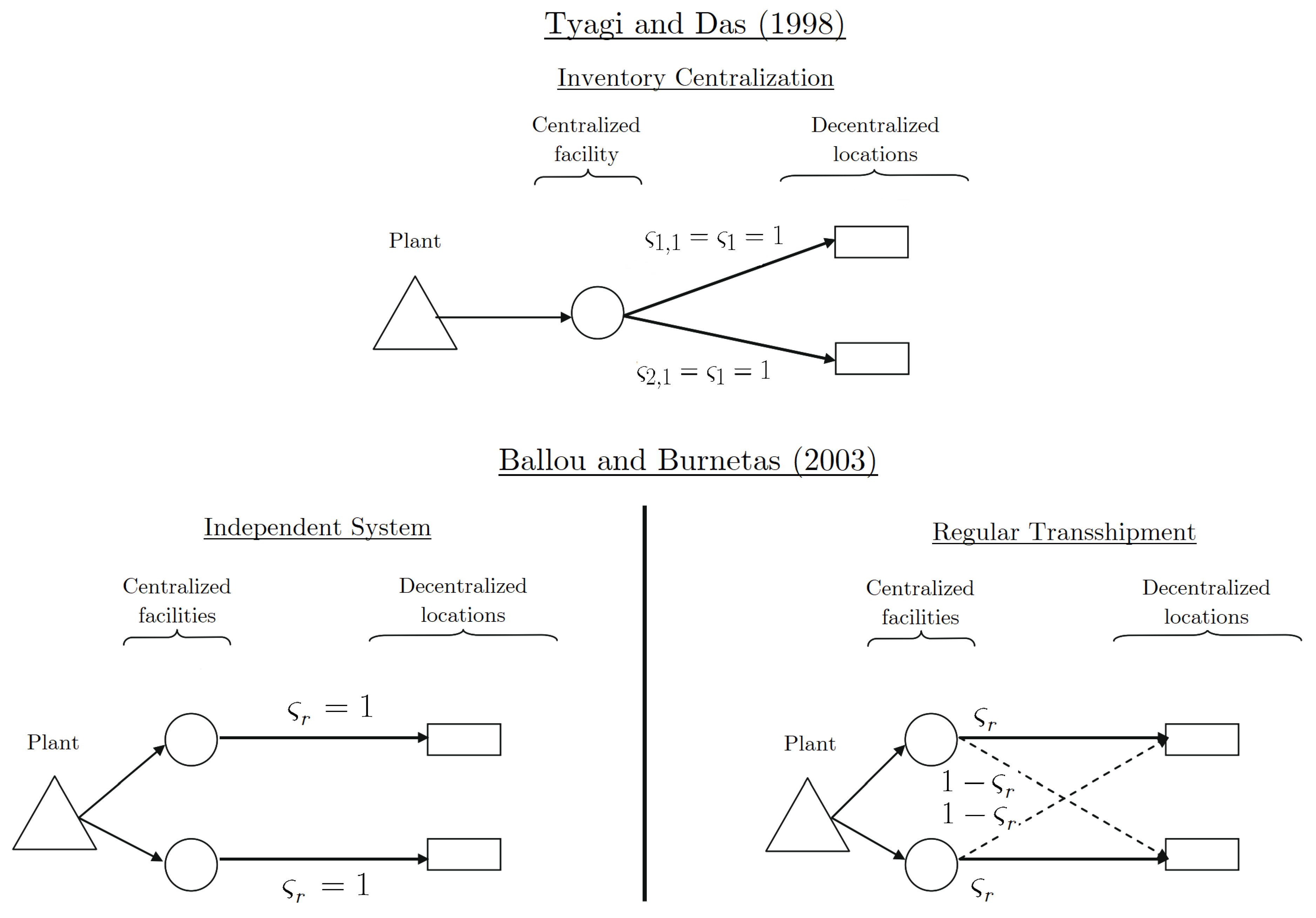
We show the case of m = n = 2 to provide a basis to compare performance. However, it may be generalized to any m and n, where m n , following the works presented in [4,5,6,11]. If  n = m = 2 , the TD rule gives ς 1 , f = ς 2 , f = ς f , for  0 ς f 1 , with  f = 1 m ς f = 1 and ς 2 = 1 ς 1 . Nonetheless, according to the BB rule, a centralized facility f provides equal demand to its main decentralized site j (that is, ς 1 , 1 = ς 2 , 2 = ς r ; ς 1 , 2 = ς 2 , 1 = 1 ς r ), where r is the site with the largest portion of the demand.
The optimal solution using the BB rule is not only different from the optimal solution obtained with the TD rule, but it also leads to different combinations of inventories [6]. Under the BB rule, if the optimal solution of ς r is zero or one, the supply chain reduces to an IS with both decentralized centers attended by a dedicated facility for each one. Nevertheless, if ς r is between zero and one, RT occurs implying that all centralized sites serve both dispersed places. Under the TD rule, if  ς 1 { 0 , 1 } , decentralized sites have a single facility serving all decentralized sites. Figure 1 exemplifies the aforementioned.
When the optimal solution of ς r is zero or one (supply IS), both sites being decentralized are attended by a facility under the BB rule. Nevertheless, if  ς 1 { 0 , 1 } , decentralized sites have a single facility employing the TD rule. Moreover, if the optimum value ς r is between zero and one, RT occurs when the BB rule is utilized. This implies that all centralized sites serve both places.
Under the TD rule, intermediate values of ς 1 yield the same pattern, but they are non-optimal solutions [11]. In what follows, we state how to compute CS c , SS c , OC c and DC c , employing both allocation rules, considering the temporal dependence of the DPUTs. However, the same expressions are valid when facing IID DPUTs, but they must be adapted to the marginal variance of the DPUTs, and, therefore, of the LTDs. Then, under the TD rule, assuming the temporal dependence of Z j t on H j t at decentralized site j, formulas defined in (15)–(18) have structures stated as
SS c = k ς 1 2 j = 1 2 μ j t 2 V ( T 1 ) + ς 1 2 V j = 1 2 Z j t | H t E ( T 1 )
+ ( 1 ς 1 ) 2 j = 1 2 μ j t 2 V ( T 2 ) + ( 1 ς 1 ) 2 V j = 1 2 Z j t | H t E ( T 2 ) ,
CS c = j = 1 2 μ j t 2 HC OC 1 ς 1 + OC 2 ( 1 ς 1 ) ,
OC c = OC 1 ς 1 ( μ 1 t + μ 2 t ) 2 CS c + OC 2 ( 1 ς 1 ) ( μ 1 t + μ 2 t ) 2 CS c ,
DC c = DC T 1 , 1 μ 1 t + DC T 1 , 2 μ 2 t ,
with μ 1 t , μ 2 t being formulated as in (4), and 
V Z 1 t + Z 2 t | H t = V ( Z 1 t | H 1 t ) + V ( Z 2 t | H 2 t ) + 2 ϱ Z 2 t , Z 1 t | H t V ( Z 1 t | H 1 t ) V ( Z 2 t | H 2 t ) .
We assume that the inventory is consolidated at site 1 to compute DC c . Under the BB rule, considering the temporal dependence of Z j t on H j t at decentralized site j, (15)–(18) take, respectively, the forms given by
SS c = k ( ( ( ς r μ 1 t + ( 1 ς r ) μ 2 t ) 2 V ( T 1 ) + ( ς r 2 V ( Z 1 t | H 1 t ) + ( 1 ς r ) 2 V ( Z 2 t | H 2 t ) . + 2 ϱ Z 2 t , Z 1 t | H t V ( Z 1 t | H 1 t ) V ( Z 2 t | H 2 t ) ς r ( 1 ς r ) ) E ( T 1 ) ) ) 1 / 2 + k ( ( ( ( 1 ς r ) μ 1 t + ς r μ 2 t ) 2 V ( T 1 ) + ( ( 1 ς r ) 2 V ( Z 1 t | H 1 t ) . + ς r 2 V ( Z 2 t | H 2 t ) 2 ϱ Z 2 t , Z 1 t | H t V ( Z 1 t | H 1 t ) V ( Z 2 t | H 2 t ) ς r ( 1 ς r ) ) E ( T 2 ) ) ) 1 / 2 ,
CS c = 1 2 HC OC 1 ( ς r μ 1 t + ( 1 ς r ) μ 2 t ) + OC 2 ( 1 ς r ) μ 1 t + ς r μ 2 t ,
OC c = OC 1 μ 1 t ς r μ 2 t ( ς r 1 ) 2 CS c + OC 2 ς r μ 2 t ( ς r 1 ) μ 1 t 2 CS c ,
DC c = ς r DC T 1 , 1 + ( 1 ς r ) DC T 2 , 1 μ 1 t + ς r DC T 2 , 2 + ( 1 ς r ) DC T 1 , 2 μ 2 t .
From (24), we must assume that the largest parts ς r of μ j t are provided with the smallest DC T 1 , 1 and DC T 2 , 2 .
In the case of decentralized site j, considering a supply IS, OC, CS, DC, and SS are expressed as  
SS j = k f = 1 m E ( T f ) V j = 1 n Z j t | H t + j = 1 n μ j t 2 V ( T f ) ,
CS j = OC j μ j t 2 HC , OC j = f = 1 m OC f μ j t 2 CS j , DC j = μ j DC T f , j .
As in the centralized case, formulas stated in (28) and (27) consider temporal dependence for the DPUTs. Nevertheless, the same expressions are valid when facing IID DPUTs, but they must be adapted to the marginal variance of the DPUTs, and therefore of the LTDs.
Thus, the objective function for a centralized system to be minimized is stated as
TC c = HC ( CS c + SS c ) + DC c + OC c ,
under the TD rule, that is, for an IC. In contrast, the objective function under a supply IS for site j is given by
TC j = HC ( CS j + SS j ) + DC j + OC j , j { 1 , 2 } ,
where the cost coefficients of a centralized system are given in (19)–(22) for the TD rule, in (24)–(26) for the BB rule, and in (29) and (30) for decentralized site j. As the objective is to determine which IC, IS or RT reduces the costs, the decision variables are related to the proportion of demand to be assigned at each site, that is, to find the optimal values of ς j , f in the TD rule, and the optimal values of ς r for the BB rule.
Following the approach given in [13], we state a consolidation effect metric associated with “the percentage reduction in aggregate SS made possible by a consolidation effect of inventory from multiple locations into one location”. This inventory metric for site j is presented as
CM j = 1 CS c + SS c CS j + SS j , j { 1 , , n } .
Figure 2 shows a flow diagram of the methodology proposed in Section 2.

3. Simulation and Analysis of Results

The new methodology stated in the current investigation is evaluated by employing simulations. In this section, we detail our computational setting and different scenarios.

3.1. Computational Setting and Simulation Framework

We use the R software to implement the proposed methodology (www.R-project.org, accessed on 29 June 2020). For the employment of the R language in inventory structures, see [14,29,30,31]. We employ the copula package of R to construct the joint distribution of the DPUTs [32]. This package provides us with the most popular copulas like Archimedian, elliptical, and Gaussian, permitting us to simulate correlated random numbers and fit a copula by goodness-of-fit methods. A generator of bivariate time series described by an ARMA model was programmed by the authors in R code and is available upon request. In addition, the generation of random numbers from bivariate ARMA models also was carried out with R codes, implemented by the authors, and available under request. We use the nloptr package of R to optimize the inventory TC of pooling models. Again, we simulate the scenario m = n = 2 , which may be generalized to other values such as m n .
The simulation considers inventory policies related to allocation and supply; modeling of the DPUT under independent and dependent cases; and optimization of costs using mathematical programming [33,34,35,36]. First, for inventory policies, we utilize three types of supply (IS/RT/IC) and two allocation rules (TD/BB). Second, the statistical models consider IID DPUTs and temporal dependence by an ARMA structure. We assume several ARMA temporal structures with bivariate normal distributions for the DPUT, whereas the IID framework is studied under marginal normal distributions. In addition, diverse simulated scenarios for mean, SDs, and correlations are considered to generate both types of DPUTs (independent and dependent) in this statistical modeling. The parameters are uniformly distributed into [ a , b ] , denoted as U [ a , b ] , which are chosen from values obtained from the literature; see, for example, Table 2 and Appendix C of [11].
Following the analysis done in [6], we contrast IC and supply IS under the TD rule based on the expressions given in (29) and (30), respectively, but assuming temporal dependence for the DPUT, which we called Case A. Moreover, the simulation examines the supply IS, IC, and RT as shown in [6], using the inventory TC defined as
TC c = HC ( CS c + SS c ) + DC c ,
under both the TD and BB rules. In this case, we consider the formula stated in (32) as the objective function to be optimized in a mathematical program and compare it to the optimization of the function defined in (30), which we name Case B.
Note that the TC c given in (29) is conformed by CC1 to CC4, whereas that the TC c stated in (32) considers CC1, CC2, and CC3. Similarly for TC j formulated in (30), under both IID DPUTs and temporal structure, the components of costs considered are the same. We consider 10,000 random scenarios for m = n = 2 minimizing the corresponding TC. Then, we obtain the optimal values of CC1 to CC4. The metrics of the simulation are detailed in Table 1.
Remark 3. 
Similar metrics are used for the IID framework, but discarding the ARMA parameters and past data. Also, σ Z 1 t , σ Z 2 t U ( 3 , 30 ) , whose values were taken from [6,11].

3.2. Simulation Study I

We examine which supply system yields the smallest costs in the 10,000 scenarios for Cases A and B, as well as independent and dependent frameworks of DPUT. The TC defined in (29) and (32) for Cases A and B, respectively, are the smallest ones under an IC. We obtain 8621 optimal scenarios recommended an IC, and 1379 scenarios with a supply IS as the best solution for Case A under an IID DPUT. Also, we attain 8628 scenarios deciding an IC as optimal supply, and 1372 scenarios with a supply IS for Case A with temporal dependence on DPUT. In Case B with IID DPUT, we reach 8912, 444, and 644 optimal values for IC, RT, and supply IS, respectively. Under temporal dependence on DPUT, the results are 8889, 697, and 414, respectively.
For the 10,000 simulations performed, we compared the number of occasions in which cost minimization was given by an IC, RT, or IS, both for the model under the assumption of an IID DPUT and for the case where it is taken into account a time-dependent DPUT. For this experiment, for each of the possible decision-making (IC, RT, IS), we applied the χ 2 test for the difference in proportions between the model considering IID DPUT and DPUT with time-dependence. The results showed a slight difference only in the case of the proportion of occasions in which the respective models opted for the choice of an IS. For this particular analysis, we detected a difference with a statistical significance of 13% (which can be considered non-significant). The above results indicate that the temporal dependence of the DPUTs reduces the TC with the supply IS according to Case B. This finding is explained by the fact that the variances of the DPUTs conditional on past data are less than for IID DPUTs, as indicated in Remarks 1 and 2.
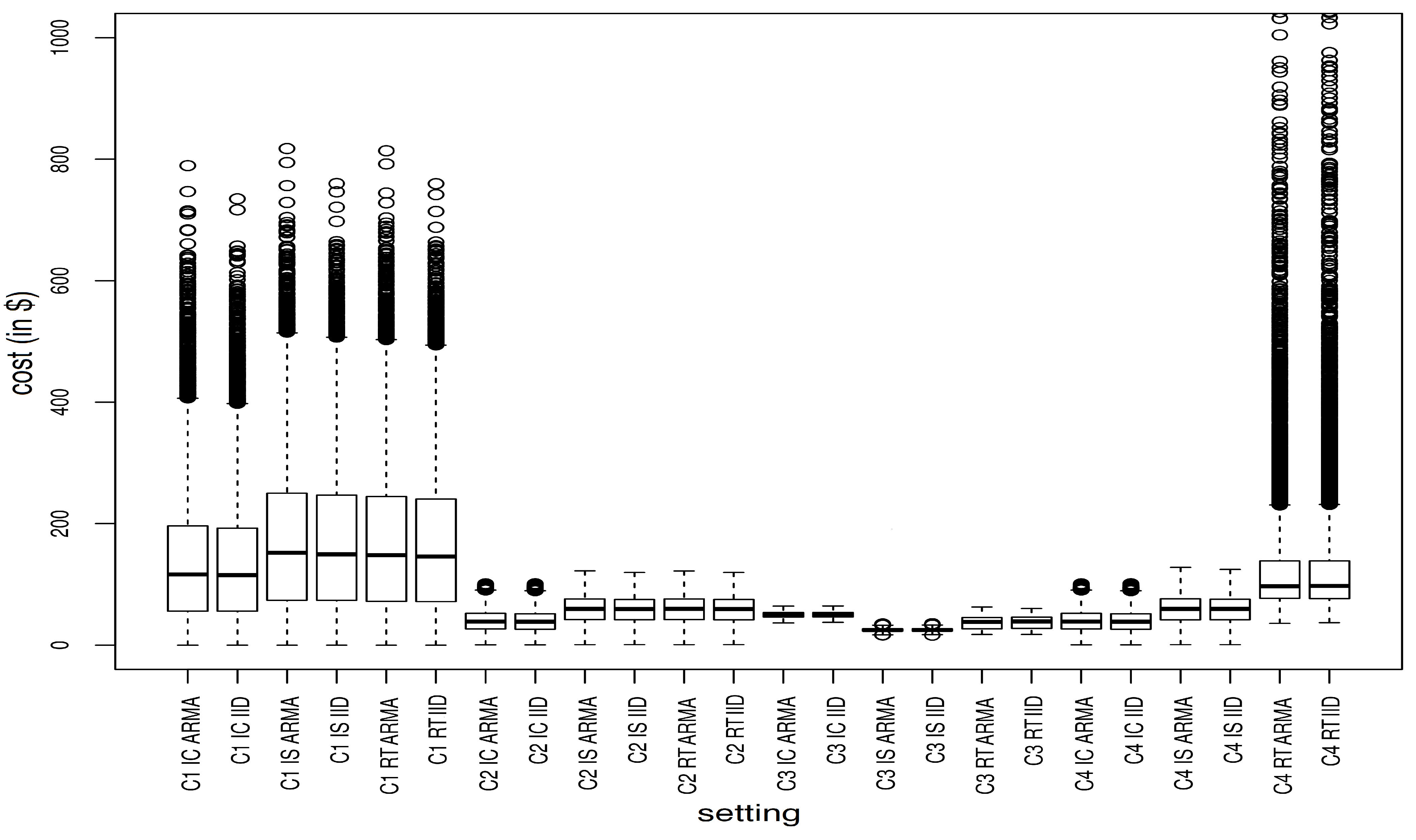
For the 10,000 scenarios under both IID and dependent frameworks, we statistically compare the parts of CC1 to CC4 of the TC for IC, RT, and supply IS. As mentioned, note that Case B analyses the four cost components CC1-CC4, while Case A only considers CC1-CC3. To graphically compare these cost components between the combinations of IC, RT or IS supply, and IID or ARMA DPUT, we show the distribution of the corresponding cost values in Figure 3. From this figure, we can see that component CC1 has the largest median cost. For the dependent framework, we analyzed the number of scenarios with CC1 as the higher cost than the other components, with 6347, 7721, and 8858 cases for RT, IC, and supply IS in Case B. We found similar results under IID DPUTs. Furthermore, the cost values of CC1-CC4 were again tested using a χ 2 statistic for differences on proportions. Significant differences were detected in favor of CC1 under IC, RT, and supply IS, for DPUTs using both with or without time-dependence frameworks. Therefore, we detected CC1 as the crucial component of the TC. Similar results were found for cases A by comparing CC1-CC3. Then, we used the Wilcoxon statistic to test the medians of the costs associated with CC1 obtained by IC, RT, and supply IS for DPUTs considering frameworks with or without time-dependence. We conclude that there are no statistically significant differences at 10% between medians for components of TC under both frameworks.
As in [14], we used the Kruskal-Wallis (KW) statistic to test medians of metrics associated with statistical parameters, costs, and safety factors regarding IC, RT, and supply IS. This test is performed if a minimal TC is attained in Cases A (IC/supply IS) and B (IC/RT/supply IS), verifying how these metrics change between DPUTs with and without temporal structure. Table 2 and Table 3 report this comparison for Cases A and B.
We observe that the medians of ϱ Z 1 , Z 2 , ϱ Z 1 t , Z 2 t | H t , σ Z 1 , σ Z 2 , σ Z 1 t | H t and σ Z 2 t | H t are related to a decrease in the TC for Case B; see Table 3. Positive correlations and low variability of the demand are linked to the supply IS, validating what was reported in [6], but now with temporal dependence for DPUTs. However, as pointed out, this dependence causes a decrease in the medians of correlations and variances of the DPUTs, when they are conditional on past data.
Table 2 and Table 3 show that it is not possible to observe significant statistical associations for medians of the ARMA parameters ( ϕ , ϑ ) in Cases A and B. As stated in Section 2, such parameters affect the correlations and conditional variances of DPUTs on past data, which are components of SS c and SS j . Table 4 reports the medians of some parameters that favor supply IS, RT, and IC for CC 1 = HC × SS . We think the temporal dependence favors lower CC 1 with RT systems concerning the TC stated under the expression stated in (32), which better balances the conditional variances of the DPUTs. Note that ϱ Z 1 t , Z 2 t | H t cannot be highly negative for obtaining a low CC 1 in IC. In addition, ϱ Z 1 t , Z 2 t | H t increases to high positive values favoring a low CC 1 in the supply IS, and slightly negative values to reach lower CC 1 in the RT. Slightly negative values of the AR parameter ϕ favor an IC, moderately positive values favor a supply IS, and values close to zero favor the RT. The MA coefficients ϑ close to zero favor an IC, moderately positive values favor a supply IS, and slightly negative values favor an RT.

3.3. Simulation Study II

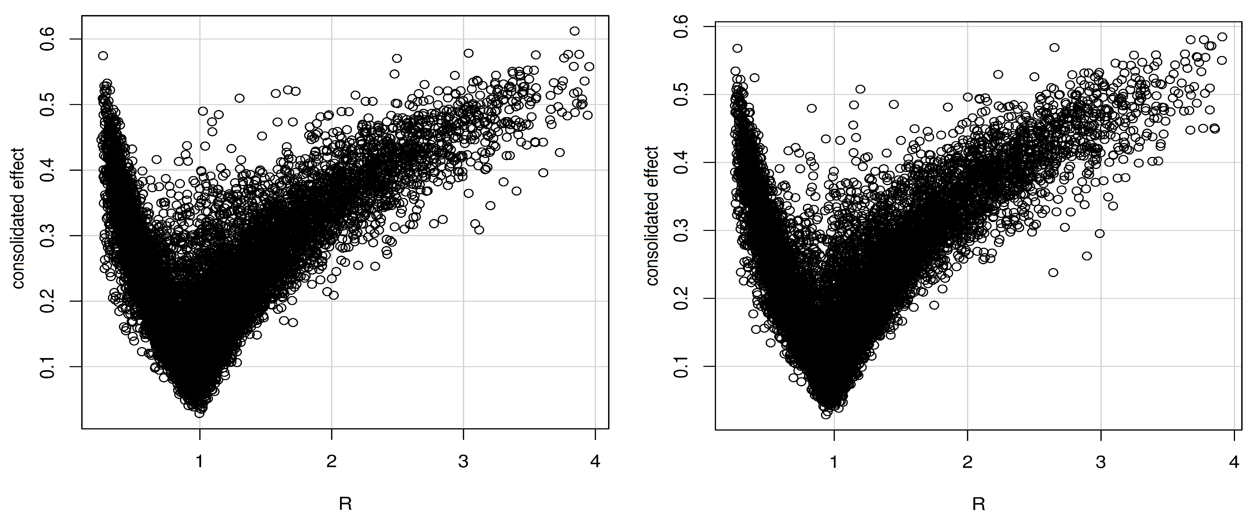
According to [6], the consolidated effect metric formulated in (31) may be a response variable modeled by a linear function of R = V ( T 2 ) / V ( T 1 ) . From the scatter-plots of Figure 4 with (left) independent and (right) dependent frameworks for the DPUTs, note that approximately linear forms are identified. Then, we consider a linear regression model to analyze the behavior of the consolidated effect metric. The estimated regression coefficients, standard errors, and t-test p-value, with temporal dependence for both R > 1 and R < 1 , related to the consolidation effect, are reported in Table 5.
Comparing the regressions obtained with R > 1 and R < 1 in Table 5, note that both coefficients of the intercept, μ 2 t , OC 2 and σ T 2 decrease and maintain their significance, while the coefficients of μ 1 t , OC 1 and σ T 1 increase keeping their significance. First, the regression coefficients of σ Z 1 t | H t and μ T 2 decrease in magnitude and significance, when R > 1 and R < 1 are compared, whereas an opposite result occurs with σ Z 2 t | H t and μ T 1 . Second, the regression coefficients of the distribution costs ( DC T 1 , 1 DC T 2 , 2 , DC T 1 , 2 , DC T 2 , 1 ), as well as the AR ( ϕ 1 , ϕ 2 ) and MA ( ϑ 1 , ϑ 2 ) coefficients, are not significant in all cases. Third, the coefficient of ϱ Z 1 t , Z 2 t | H t maintains its magnitude and significance with R > 1 and R < 1 , whereas its R-squared coefficients are similar. An analogous analysis without time-dependence can be consulted in Table 7 of [6].

4. Empirical Application and Implications

This section applies our methodology to real data and provides management implications in decision making.

4.1. Illustrative Example

To illustrate our methodology, we apply it to real data taken from kaggle.com/c/competitive-data-science-predict-future-sales (accessed on 29 June 2020).
The data correspond to sales of one of the biggest software firms in Russia named 1C Company. This data set is free to utilize for any purpose, including commercial use. We employed the total monthly sales over 24 months for the product with the highest demand in Moscow. The identifier of this product is ID 20949.
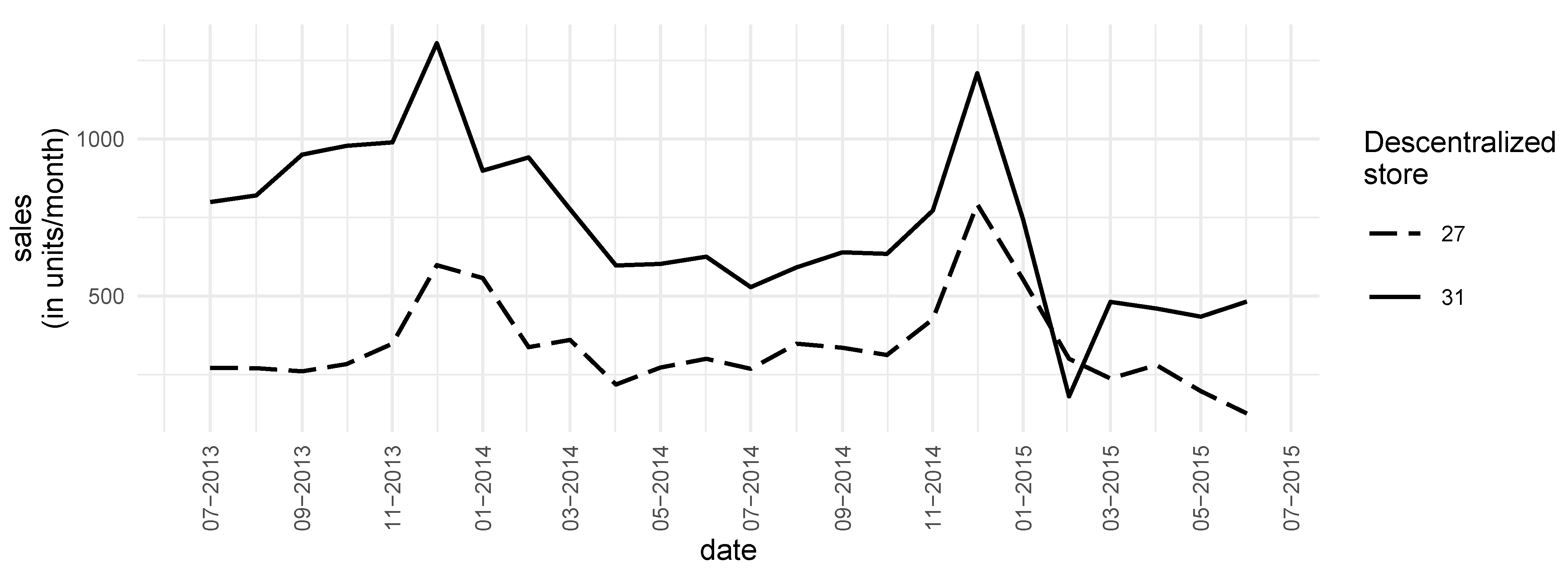
We considered the two demand points that contain sufficient history to fit an ARMA model: the demand points #27 and #31. We call these demand points the decentralized stores. The data considered are shown in Table 6 and graphically represented in Figure 5. Descriptive statistics for both demand points are detailed in Table 7. From this table, graphically supported by Figure 5, note that demand point #31 has demand mean and SD greater than stock point #27. Plots of the autocorrelation function (ACF) and partial ACF (PACF) are simple techniques to find temporal DPUT patterns. The reader is suggested to see [28] for an explanation of these graphical plots. To check the temporal dependence of sales, we used the ACF and PACF for both demand points #27 and #31. Their graphical plots are shown in Figure 6, which suggest time-dependence in both time series. Given this result, we utilized the forecast library of the R software with its auto.arima function to fit an ARMA model and estimate its order as well as its parameters. Also, we used the Akaike information criteria (AIC) to select the better model, where a less value of AIC indicates a better fit of the model. The results coincide with the recommendation provided in Figure 6, since the fitted ARMA models are AR( ϕ = 0.59 ) and MA( ϑ = 0.69 ) for demand points #27 and #31, respectively. Furthermore, the estimated SDs conditioned on past data are 118.88 and 211.12 units, respectively.
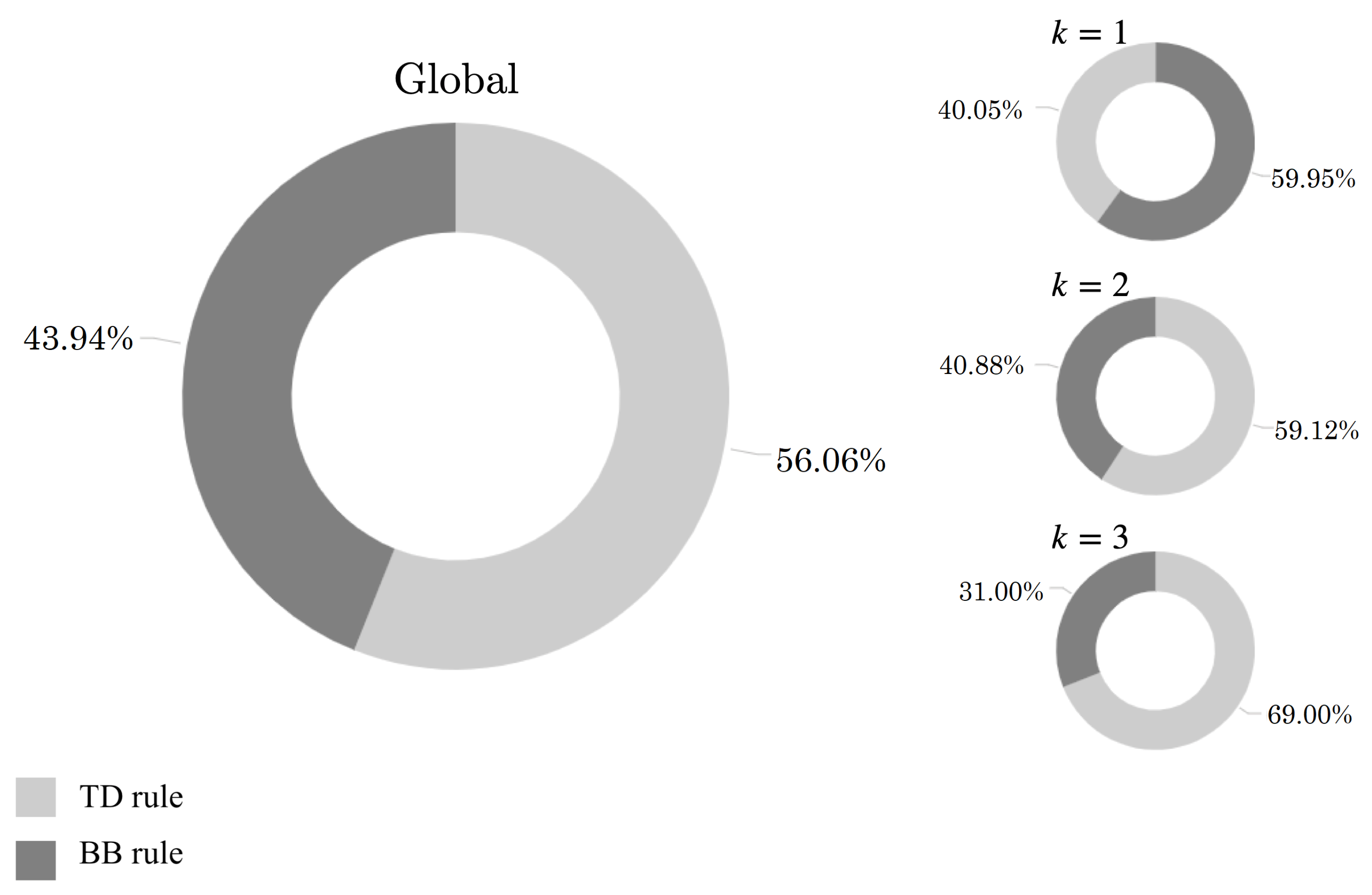
To evaluate the behavior of our model, we considered low, medium, and high values for the cost parameters of the proposed model, employing the metrics detailed in Section 3.1. Following [6], we stated the safety factor parameter: k { 1 , 2 , 3 } ; OC: OC 1 { 20 , 40 , 60 } and OC 2 { 20 , 80 , 140 } ; mean LTs: LT 1 = LT 2 { 1 , 3 , 5 } ; and SDs: S LT 1 = S LT 2 { 0.5 , 1 , 2 } . The proposed model was implemented for all possible combinations. The TCs were evaluated under the TD and BB rules and compared with TC under an IS. In this experiment, overall, 56.06% of the occasions have lower TC under the TD rule, while in 43.9% of the cases, the best decision was the BB rule. There are no lower TC under the IS. One of the most interesting findings resides in the choice of k. It is expected that, as k increases, the TC increases as well, regardless of the evaluated system. However, when k = 1 , most decisions minimizing costs were made under the BB rule. In other cases, when k { 2 , 3 } , the TD rule minimized the costs in 59.12% and 69% of the cases, respectively. These results are shown in Figure 7.
Without loss of generality, when the choice is to centralize, the inventories are consolidated in location 1. Unsurprisingly, such a choice tends to be made when OCs for that centralized location are lower, while OCs for the second centralized location are high. No significant differences were observed concerning the average LT.
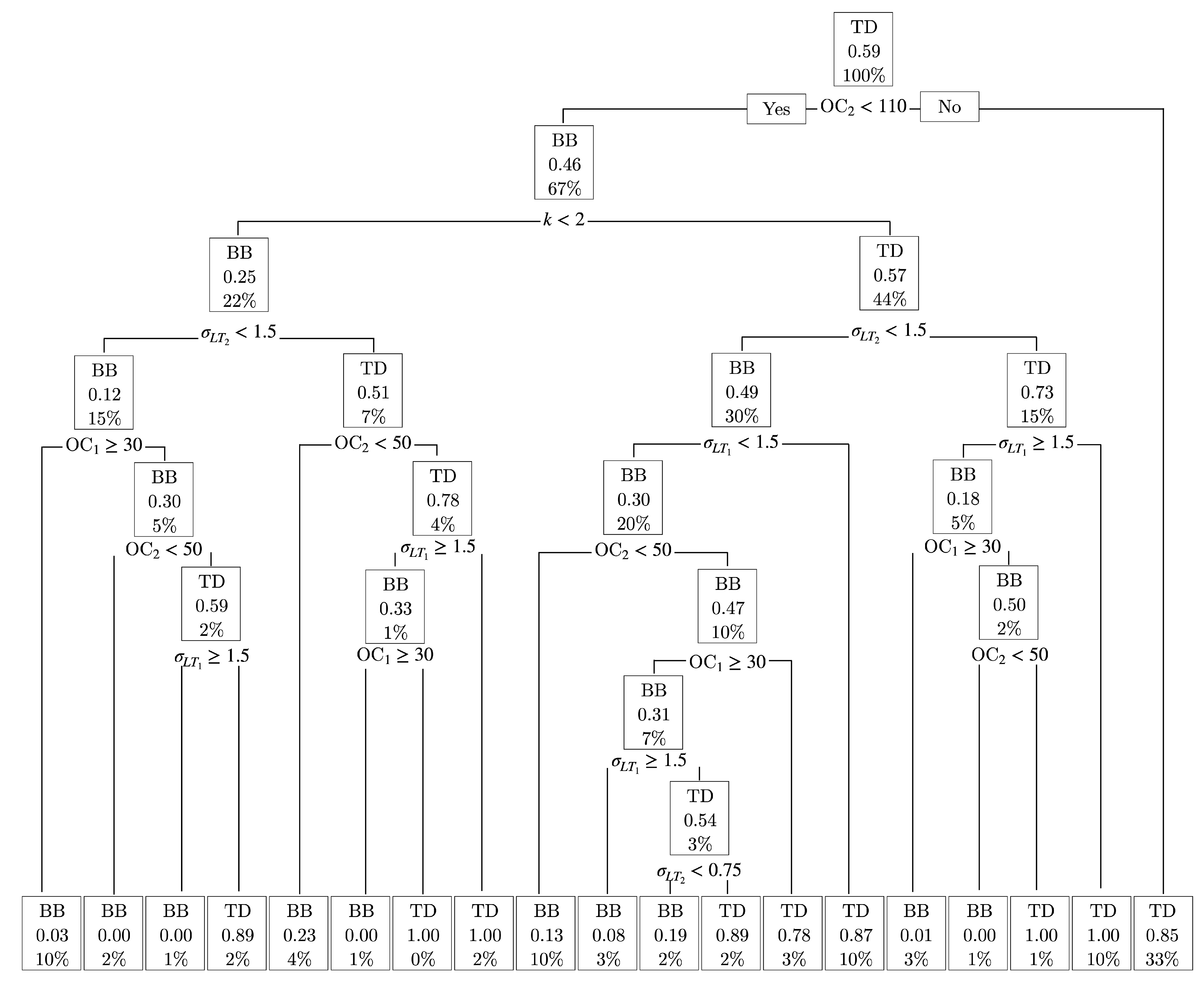
Nevertheless, it is possible to notice that, when the variability of the LT in centralized location 1 is low compared to the variability of the LT of location 2, the best decision also tends to make centralization in one location. Then, we applied a decision tree using the R software to detect deep patterns in the decision framework. Figure 8 shows the corresponding results. From this plot, we can observe that most decisions are related to LT and variability of the SS. Furthermore, we can observe a particular case when the OC 1 is high with low OC 2 . Then, the decision is to apply a centralization under the TD rule. This is expected because this allocation rule centralizes the inventories mainly in one dedicated facility. In this specific case, the solution is centralized in the facility with lower OC, that is, location 1, except for the presence of a high LT variance for facility 1 and lower LT variance for facility 2. In the case of the IID framework, the results are very similar. Note that examination of Figure 8 and Figure 9 shows that the safety factor is more critical. We can notice that there are no different patterns.

4.2. Implications in Management

Following the analysis done in [14], we explain the consequences of the obtained findings for logistics management when decision making. First, when inventory consolidation is desired, it is critical to understand the temporal patterns that DPUT data might have. We conclude from our results that these temporal patterns directly affect the metrics associated with the correlation and variance of the demand when historical data are included. These metrics directly influence component CC1 of the inventory TCs, which is the essential component in all pooled inventory and supply IS strategies; see Figure 3. Next, some of the main implications are provided:
  • When facing DPUTs with a temporal structure, the supply IS is favored as it is related to decreasing variances and correlations conditioned on past data.
  • IID DPUTs favor IC systems with an increase of the HC of CS .
  • Temporal dependence favors lower CC 1 with RT systems.
  • The metrics with a high effect on percentual consolidate effect for R > 1 are ordered as: σ T 2 > HC > k > ϱ Z 1 t , Z 2 t | H t > OC f > μ Z t > μ T > V ( Z t | H t ) .
  • The metrics with a high effect on the percentual consolidate effect for R < 1 are: σ T 2 > ϱ Z 1 t , Z 2 t | H t > OC f > μ T > μ Z t > HC > V ( Z t | H t ) > k .
As explained at the end of Section 3.2, one of our findings is that the medians of ϱ Z 1 t , Z 2 t | H t associated with IC and supply IS is less than ϱ Z 1 , Z 2 . This finding can be explained because ϱ Z 1 t , Z 2 t | H t should be regulated by the temporal structure described by the parameters ϕ and ϑ . Then, we propose regressions, for  R > 1 and R < 1 , between the response variable related to the consolidate effect and ϱ Z 1 t , Z 2 t | H t , as well as with other covariates conditional on given values of Φ = ϕ and ϑ = ϑ , to establish when this regulation is greater or less. These results are shown qualitatively for better comprehension in Table 8, in which the regulation effect of the temporal structures is given in intervals for parameters Φ and ϑ , indicating that this effect goes from more to less according to the notation + + + > + + > + > . Recall that the IC is associated with ϱ Z 1 t , Z 2 t | H t < 0 , and its regulations are considered more significant to favor the IC, while the corresponding regression coefficient is more negative.
From the analysis provided in Table 4, it is essential to highlight some differences that occur when comparing the medians of the ARMA metrics. These metrics are associated with the different supply systems that decrease CC1. There, models with pure positive AR coefficients (without considering the MA part) or positive coefficients of pure MA (without considering the AR part) would be more associated with an IS supply. This generates visible “wave” patterns, which would be related to the IS supply. In addition, coefficients of positive MA are related to upward trends of the time series, which would be associated with an IS supply as well. In the case of positive AR models, the consecutive residuals share similar values and signs, showing large areas of overestimation and underestimation.

5. Discussion, Concluding Remarks, Limitations, and Further Work

In this section, we discuss our investigation and provide conclusions, limitations, and ideas for further research.

5.1. Discussion

Our findings suggest new decision-making patterns to be considered in comparison with previous works. We model the temporal disposition of demand data, due to its effect on the variance conditional on past data. This effect suggests that the rule with the best behavior is a pooled inventory in the safety stock that was consolidated, which is obtained by multiplying with the holding cost and then by the total cost.
Specifically, given that safety stocks increase as the variance is greater, the existence of temporary structures for demand data under an ARMA model implies lower levels of safety stocks, due to the conditional demand overtime on the data is less than the marginal variances typically assumed under an approach of independent and identically distributed random variables. Regarding the total cost, we suggest selecting dedicated facilities for supply. Regular transshipment outperformed the independent supply system statistically for the component associated with the safety stock that was consolidated, which is multiplied by the holding cost.
We detect that when the demand per unit of time of different decentralized sites has low variance and positive correlation among them, an independent system is usually the best option to consider in the supply chain. This result is consistent with the conclusions given in [6] for an independent and identically distributed random demand, but now studied in a time-dependent framework.

5.2. Conclusions

In this study, we have analyzed the effect of consolidation on inventory costs compared to a system without consolidation. We have formulated an inventory structure based on continuous-review using allocation rules for regular transshipment and centralization, which has established temporal structures of demand. Our methodology proposed in this work was implemented in R language developed by the authors, which is available to the readers upon request. This allowed us to conduct simulations employing synthetic data with and without autoregressive moving average structures and to prove our model under a real-world data scenario. Numerical simulations have demonstrated that, under time-dependence, the conditional demand variance, based on past data, is less than the marginal variance. Our finding favors dedicated locations for inventory replenishment. In addition, temporal structures have reduced the costs of maintaining safety stocks through regular transshipments when such temporal patterns exist. These results have been also illustrated in an example employing real-world data.
In summary, in the previous research [11,14,16,17,18,19,21] to our study, such as was warned in [22], there was a gap on inventory models under consolidation effects between those that incorporate temporal dependence and those that do not. In this context, one of the few works on consolidation effects in inventory models is [23], while in [24], optimal policies were proposed for inventories with temporally correlated demand in a similar setting, although not on the consolidation impact. In the present study, we have covered such a gap. Our investigation has provided essential information for managing supply chains in the presence of time-patterned demands. These findings are of interest to decision-makers in the supply chain.

5.3. Limitations and Future Research

Although this work considers a critical aspect, such as the time-dependence on the demand, one of its limitations is the assumption of a Gaussian distribution, which is usually violated in practice. To address this problem, this work may be expandable to more general models, for example, to the largely known generalized linear modeling. This type of model is widely flexible, permitting functional forms that may be linear and non-linear [37]. Furthermore, probability distributions different from the Gaussian or normal model can be considered this kind of statistical model assumed for the demand, enabling other shapes of the demand statistical distribution to be assumed [31]. Moreover, multivariate distributions may also be considered [38]. It is essential to state these new statistical methods when studying a cost reduction through the use of locations for facilities of consolidation, which combine diverse shipments enhancing the service level [12]. These ideas are being explored by the authors and their findings will be documented in new publications. Other directions and applications on our proposal are presented in [39,40,41,42,43].

Author Contributions

Conceptualization: M.H., V.L., F.R., P.W. and X.C. Data curation: M.H., V.L. and F.R. Formal analysis: M.H., V.L. and F.R. Investigation, M.H., V.L., F.R., P.W. and X.C. Methodology: M.H., V.L., F.R., P.W. and X.C. Writing—original draft: M.H., F.R., P.W. and X.C. Writing—review and editing: V.L. All authors have read and agreed to the published version of the manuscript.

Funding

This research was partially funded by FONDECYT, project grants number 1200525 (V.L. and M.H.) and 11190004 (F.R.) from the National Agency for Research and Development (ANID) of the Chilean government under the Ministry of Science, Technology, Knowledge and Innovation.

Institutional Review Board Statement

Not applicable.

Informed Consent Statement

Not applicable.

Data Availability Statement

The data and codes used in this study are available under request.

Acknowledgments

The authors would like to thank the Editors and four reviewers for their constructive comments which led to improvement in the presentation of the manuscript.

Conflicts of Interest

The authors declare no conflict of interest.

References

  1. Chopra, S. Designing the distribution network in a supply chain. Transp. Res. Part Logist. Transp. Rev. 2003, 39, 123–140. [Google Scholar] [CrossRef]
  2. Farahani, R.Z.; Elahipanah, M. A genetic algorithm to optimize the total cost and service level for just-in-time distribution in a supply chain. Int. J. Prod. Econ. 2008, 111, 229–243. [Google Scholar] [CrossRef]
  3. Laporte, G.; Nickel, S.; Saldanha-da-Gama, F. Location Science; Springer: Berlin, Germany, 2019. [Google Scholar]
  4. Ballou, R.H.; Burnetas, A. Planning multiple location inventories. J. Bus. Logist. 2003, 24, 65–89. [Google Scholar] [CrossRef]
  5. Tyagi, R.; Das, C. Extension of the square root law for safety stock to demands with unequal variances. J. Bus. Logist. 1998, 19, 197–203. [Google Scholar]
  6. Wanke, P. Consolidation effects and inventory portfolios. Transp. Res. Part Logist. Transp. Rev. 2009, 45, 107–124. [Google Scholar] [CrossRef]
  7. Berman, O.; Krass, D.; Tajbakhsh, M. On the benefits of risk pooling in inventory management. Prod. Oper. Manag. 2011, 20, 57–71. [Google Scholar] [CrossRef]
  8. Evers, P.T. The impact of transshipments on safety stock requirements. J. Bus. Logist. 1996, 17, 109–127. [Google Scholar]
  9. Schmitt, A.J.; Sun, S.A.; Snyder, L.V.; Shen, Z.M. Centralization versus decentralization: Risk pooling, risk diversification, supply chain disruptions. Omega 2015, 52, 201–212. [Google Scholar] [CrossRef]
  10. Evers, P.T.; Beier, F.J. The portfolio effect and multiple consolidation points: A critical assessment of the square root law. J. Bus. Logist. 1993, 14, 109–125. [Google Scholar]
  11. Wanke, P. Consolidation effects: Assessing the impact of tail dependence on inventory pooling using copulas. Int. J. Inventory Res. 2014, 2, 174–188. [Google Scholar] [CrossRef]
  12. Askin, R.G.; Baffo, I.; Xia, M. Multi-commodity warehouse location and distribution planning with inventory consideration. Int. J. Prod. Res. 2014, 52, 1897–1910. [Google Scholar] [CrossRef]
  13. Tallon, W.J. The impact of inventory centralization on aggregate safety stock: The variable supply lead time case. J. Bus. Logist. 1993, 14, 87–100. [Google Scholar]
  14. Rojas, F.; Leiva, V.; Huerta, M.; Martin-Barreiro, C. Lot-size models with uncertain demand considering its skewness/kurtosis and stochastic programming applied to hospital pharmacy with sensor-related COVID-19 data. Sensors 2021, 21, 5198. [Google Scholar] [CrossRef] [PubMed]
  15. Rojas, F.; Wanke, P.; Bravo, F.; Tan, Y. Inventory pooling decisions under demand scenarios in times of COVID-19. Comput. Ind. Eng. 2021, 161, 107591. [Google Scholar] [CrossRef]
  16. Corbett, C.J.; Rajaram, K. A generalization of the inventory pooling effect to nonnormal dependent demand. Manuf. Serv. Oper. Manag. 2006, 8, 351–358. [Google Scholar] [CrossRef]
  17. Derbel, M.; Hachicha, W.; Aljuaid, A.M. Sensitivity analysis of the optimal inventory-pooling strategies according to multivariate demand dependence. Symmetry 2021, 13, 328. [Google Scholar] [CrossRef]
  18. Yang, C.; Hu, Z.; Zhou, S.X. Multilocation newsvendor problem: Centralization and inventory pooling. Manag. Sci. 2021, 67, 185–200. [Google Scholar] [CrossRef]
  19. Zhi, B.; Wang, X.; Xu, F. Portfolio optimization for inventory financing: Copula-based approaches. Comput. Oper. Res. 2021, 136, 105481. [Google Scholar] [CrossRef]
  20. Calfa, B.A. Data Analytics Methods for Enterprise-Wide Optimization under Uncertainty. Doctoral Dissertation, Carnegie Mellon University, Pittsburgh, PA, USA, 2015. [Google Scholar]
  21. Box, G.E.P.; Jenkins, G.M.; Reinsel, G.C.; Ljung, G.M. Time Series Analysis: Forecasting and Control; Wiley: Hoboken, NJ, USA, 2015. [Google Scholar]
  22. Williams, W.; Peters, M.; Raiszadeh, M. Time-dependent demand in requirements planning: An exploratory assessment of the effects of serially correlated demand sequences on lot-sizing performance. J. Oper. Manag. 1985, 6, 69–85. [Google Scholar] [CrossRef]
  23. Erkip, N.; Hausman, W.; Nahmias, S. Optimal centralized ordering policies in multi-echelon inventory systems with correlated demands. Manag. Sci. 1990, 36, 381–392. [Google Scholar] [CrossRef]
  24. Dong, L.; Lee, H.L. Optimal policies and approximations for a serial multiechelon inventory system with time-correlated demand. Oper. Res. 2003, 51, 969–980. [Google Scholar] [CrossRef] [Green Version]
  25. Li, C.; Fang, X.; Yan, Z.; Huang, Y.; Liang, M. Research on gas concentration prediction based on the ARIMA-LSTM combination model. Processes 2023, 11, 174. [Google Scholar] [CrossRef]
  26. Benjamin, M.A.; Rigby, R.A.; Stasinopoulos, D.M. Generalized autoregressive moving average models. J. Am. Stat. Assoc. 2003, 98, 214–223. [Google Scholar] [CrossRef]
  27. Rojas, F.; Leiva, V.; Wanke, P.; Lillo, C.; Pascual, J. Modeling lot-size with time-dependent demand based on stochastic programming and case study of drug supply in Chile. PLoS ONE 2019, 14, e0212768. [Google Scholar] [CrossRef] [Green Version]
  28. Tsay, R.S. Analysis of Financial Time Series; Wiley: Hoboken, NJ, USA, 2002. [Google Scholar]
  29. Rojas, F.; Leiva, V.; Wanke, P.; Marchant, C. Optimization of contribution margins in food services by modeling independent component demand. Colomb. J. Stat. 2015, 38, 1–30. [Google Scholar] [CrossRef]
  30. Wanke, P.; Ewbank, H.; Leiva, V.; Rojas, F. Inventory management for new products with triangularly distributed demand and lead-time. Comput. Oper. Res. 2016, 69, 97–108. [Google Scholar] [CrossRef]
  31. Wanke, P.; Leiva, V. Exploring the potential use of the Birnbaum-Saunders distribution in inventory management. Math. Probl. Eng. 2015, 2015, 827246. [Google Scholar] [CrossRef] [Green Version]
  32. Hofert, M.; Kojadinovic, I.; Maechler, M.; Yan, J. Copula: Multivariate Dependence with Copulas. R Package Version 0.999-9. 2014. Available online: http://CRAN.R-project.org/package=copula (accessed on 29 June 2023).
  33. Alkatheri, M.; Alhameli, F.; Betancourt-Torcat, A.; Almansoori, A.; Elkamel, A. Clustering approach for the efficient solution of multiscale stochastic programming problems: Application to energy hub design and operation under uncertainty. Processes 2023, 11, 1046. [Google Scholar] [CrossRef]
  34. Hillier, F.; Lieberman, G. Introduction to Operational Research; McGraw Hill: New York, NY, USA, 2005. [Google Scholar]
  35. Shapiro, A.; Dentcheva, D.; Ruszczynski, A. Lectures on Stochastic Programming: Modeling and Theory; SIAM: Philadelphia, PA, USA, 2014; Volume 16. [Google Scholar]
  36. Kall, P.; Wallace, S.W.; Kall, P. Stochastic Programming; Springer: New York, NY, USA, 1994. [Google Scholar]
  37. Leiva, V.; Santos-Neto, M.; Cysneiros, F.J.A.; Barros, M. Birnbaum-Saunders statistical modelling: A new approach. Stat. Model. 2014, 14, 21–48. [Google Scholar] [CrossRef]
  38. Marchant, C.; Leiva, V.; Cysneiros, F.J.A. A multivariate log-linear model for Birnbaum-Saunders distributions. IEEE Trans. Reliab. 2016, 65, 816–827. [Google Scholar] [CrossRef]
  39. Bhakoo, V.; Singh, P.; Sohal, A. Collaborative management of inventory in Australian hospital supply chains: Practices and issues. Supply Chain. Manag. Int. J. 2012, 17, 217–230. [Google Scholar] [CrossRef]
  40. Delgado, E.; Cabezas, X.; Martin-Barreiro, C.; Leiva, V.; Rojas, F. An equity-based optimization model to solve the location problem for healthcare centers applied to hospital beds and COVID-19 vaccination. Mathematics 2022, 10, 1825. [Google Scholar] [CrossRef]
  41. Zepeda, E.D.; Nyaga, G.N.; Young, G.J. Supply chain risk management and hospital inventory: Effects of system affiliation. J. Oper. Manag. 2016, 44, 30–47. [Google Scholar] [CrossRef]
  42. Rojas, F.; Wanke, P.; Leiva, V.; Huerta, M.; Martin-Barreiro, C. Modeling inventory cost savings and supply chain success factors: A hybrid robust compromise multi-criteria approach. Mathematics 2022, 10, 2911. [Google Scholar] [CrossRef]
  43. Raa, B.; Aghezzaf, H. A robust dynamic planning strategy for lot-sizing problems with stochastic demands. J. Intell. Manuf. 2005, 16, 207–213. [Google Scholar] [CrossRef]
Figure 1. Linking allocation rules to inventory-pooling models. Adapted from [6].
Processes 11 02008 g001
Figure 2. Flow diagram of the proposed methodology.
Processes 11 02008 g002
Figure 3. Boxplots of the indicated cost and type of dependence.
Processes 11 02008 g003
Figure 4. Scatter-plot of consolidated effect versus R = V ( T 2 ) / V ( T 1 ) for IID (left) and serial (right) DPUTs.
Processes 11 02008 g004
Figure 5. Time series plot of data set corresponding to sales of the 1C Company.
Processes 11 02008 g005
Figure 6. ACFs (left) and PACFs (right) for demand points 27 (top) and 31 (bottom).
Processes 11 02008 g006
Figure 7. Distribution of selected allocation rules which minimize the TC by all combinations of the presented experiment.
Processes 11 02008 g007
Figure 8. Tree of decision for the empirical application under a time-dependent framework.
Processes 11 02008 g008
Figure 9. Tree of decision for the empirical application under a time IID framework.
Processes 11 02008 g009
Table 1. Type of metric of the simulation study.
Statistical ParametersCosts
μ Z 1 t , μ Z 2 t U ( 80 , 120 ) DC T 1 , 1 , DC T 2 , 2 U ( 0.20 , 0.25 )
σ Z 1 t | H t U ( 3 , 30 ) DC T 1 , 2 , DC T 2 , 1 U ( 0.25 , 0.30 )
σ Z 2 t | H t U ( 3 , 30 ) × ( 1 ϱ Z 1 t , Z 2 t | H t 2 ) 1 / 2 HC U ( 1 , 1000 )
ϱ Z 1 t , Z 2 t | H t U ( 1 , 1 ) OC 1 U ( 17 , 67 )
μ T 1 , μ T 2 U ( 1 , 5 ) OC 2 U ( 20 , 140 )
σ T 1 , σ T 2 U ( 0.5 , 2 )
ARMA parametersSafety factor
ϕ 1 , ϕ 2 , ϑ 1 , ϑ 2 U ( 1 , 1 ) k U ( 1 , 3 )
Table 2. Median and KW p-value for the mentioned model, metric, and supply, employing the TC in Case A.
IID ModelARMA Model
MetricICISKW p-ValueMetricICISKW p-Value
μ Z 1 99.61102.69<0.001 μ Z 1 t 99.58101.61<0.001
μ Z 2 100.26100.420.71 μ Z 2 t 99.9099.680.37
σ Z 1 16.4116.090.44 σ Z 1 t | H t 16.4416.310.64
σ Z 2 16.6516.560.52 σ Z 2 t | H t 11.9811.970.25
ϱ Z 1 , Z 2 −0.0140.040.04 ϱ Z 1 t , Z 2 t | H t −0.0080.0340.2381
μ T 1 2.972.920.21 μ T 1 2.992.960.61
μ T 2 3.012.890.03 μ T 2 2.982.960.75
σ T 1 1.221.33< 0.001 σ T 1 1.231.33< 0.001
σ T 2 1.261.13< 0.001 σ T 2 1.271.17< 0.001
DC T 1 , 1 0.1250.1230.02 DC T 1 , 1 0.1250.1240.33
DC T 2 , 2 0.1250.1240.86 DC T 2 , 2 0.1250.1250.47
DC T 1 , 2 0.3750.3760.13 DC T 1 , 2 0.3750.3760.34
DC T 2 , 1 0.3750.3760.02 DC T 2 , 1 0.3740.3760.011
k1.991.90< 0.001 k2.011.89< 0.001
HC 0.380.048< 0.001 HC 0.380.05< 0.001
OC 1 42.3738.51< 0.001 OC 1 42.7638.47< 0.001
OC 2 80.7572.62< 0.001 OC 2 80.8771.54< 0.001
---- ϕ 1 −0.004−0.0100.87
---- ϕ 2 −0.0001−0.00240.69
---- ϑ 1 0.0010.01910.55
---- ϑ 2 −0.0030.00050.92
Table 3. Median and KW p-value for the mentioned model, metric, and supply, employing the TC in Case B.
IID ModelARMA Model
MetricICISRTKW p-ValueMetricICISRTKW p-Value
μ Z 1 99.96100.58100.140.22 μ Z 1 t 99.9099.65100.760.78
μ Z 2 100.08101.62102.080.06 μ Z 2 t 99.55103.45101.42< 0.001
σ Z 1 16.6912.0116.61< 0.001 σ Z 1 t | H t 16.8310.7817.89< 0.001
σ Z 2 16.9712.0516.850.001 σ Z 2 t | H t 12.338.4111.91< 0.001
ϱ Z 1 , Z 2 −0.050.530.06< 0.001 ϱ Z 1 t , Z 2 t | H t −0.030.420.06< 0.001
μ T 1 2.982.812.880.034 μ T 1 3.012.742.87< 0.001
μ T 2 3.022.622.94< 0.001 μ T 2 3.012.643.03< 0.001
σ T 1 1.221.361.37< 0.001 σ T 1 1.231.411.30< 0.001
σ T 2 1.251.221.140.002 σ T 2 1.251.271.190.16
DC T 1 , 1 0.1240.1240.1230.86 DC T 1 , 1 0.1240.1230.1250.38
DC T 2 , 2 0.1240.1240.1240.99 DC T 2 , 2 0.1250.1260.1240.44
DC T 1 , 2 0.3750.3760.3760.63 DC T 1 , 2 0.3750.3740.3780.012
DC T 2 , 1 0.3750.3740.3770.11 DC T 2 , 1 0.3760.3740.3760.13
k2.001.801.88< 0.001 k2.011.801.81< 0.001
HC 0.370.070.04< 0.001 HC 0.370.070.044< 0.001
OC 1 42.0739.7742.250.035 OC 1 42.2740.7341.640.21
OC 2 80.1775.4773.080.025 OC 2 80.5573.3169.54< 0.001
----- ϕ 1 −0.0080.0030.0070.36
----- ϕ 2 −0.00028−0.00980.0240.95
----- ϑ 1 0.006−0.021−0.0320.50
----- ϑ 2 0.0017−0.02−0.0470.21
Table 4. Median and KW p-value for the mentioned metric, and supply, employing an ARMA model for DPUT based on CC1.
MetricICISRTKW p-Value
σ Z 1 t | H t 16.469.4117.01< 0.001
σ Z 2 t | H t 11.978.1713.39< 0.001
ϱ Z 1 t , Z 2 t | H t −0.0010.50−0.058< 0.001
ϕ 1 −0.007−0.060.0210.570
ϕ 2 −0.0050.210.0900.007
ϑ 1 0.0020.31−0.0240.030
ϑ 2 −0.0010.01−0.0190.680
Table 5. Indicators of the t-test for the listed covariate parameter on the consolidated effect with an ARMA model utilizing DPUT and the mentioned R.
Covariate R > 1 R < 1
EstimateStandard Errorp-ValueEstimateStandard Errorp-Value
Constant 3.256 × 10 1 1.333 × 10 2 < 0.001 1.998 × 10 1 1.423 × 10 2 < 0.001
μ Z 1 t 6.482 × 10 4 2.876 × 10 5 < 0.001 3.449 × 10 4 2.995 × 10 5 < 0.001
μ Z 2 t 4.408 × 10 4 2.878 × 10 5 < 0.001 4.365 × 10 4 2.983 × 10 5 < 0.001
σ Z 1 t | H t 3.127 × 10 4 4.209 × 10 5 < 0.001 7.747 × 10 5 4.424 × 10 5 0.080
σ Z 2 t | H t 8.543 × 10 5 4.222 × 10 5 0.0431 3.036 × 10 4 4.451 × 10 5 < 0.001
ϱ Z 1 t , Z 2 t | H t 7.013 × 10 3 5.685 × 10 4 < 0.001 6.852 × 10 3 5.915 × 10 4 < 0.001
μ T 1 6.603 × 10 4 2.842 × 10 4 < 0.001 2.576 × 10 3 3.006 × 10 4 < 0.001
μ T 1 1.570 × 10 3 2.859 × 10 4 < 0.001 1.249 × 10 3 3.034 × 10 4 < 0.001
σ T 1 3.185 × 10 1 1.267 × 10 3 < 0.001 2.091 × 10 1 1.123 × 10 3 < 0.001
σ T 2 2.009 × 10 1 1.161 × 10 3 < 0.001 2.981 × 10 1 1.284 × 10 3 < 0.001
DC T 1 , 1 4.184 × 10 2 2.341 × 10 2 < 0.001 6.839 × 10 3 2.403 × 10 2 0.776
DC T 2 , 2 6.057 × 10 3 3.189 × 10 2 0.8494 4.562 × 10 3 2.397 × 10 2 0.849
DC T 1 , 2 2.424 × 10 2 2.331 × 10 2 0.2985 4.596 × 10 4 2.425 × 10 2 0.985
DC T 2 , 1 2.810 × 10 2 2.322 × 10 2 0.2263 1.952 × 10 3 2.385 × 10 2 0.935
k 2.020 × 10 2 6.098 × 10 4 < 0.001 8.566 × 10 5 6.119 × 10 4 0.889
HC 7.082 × 10 2 1.907 × 10 3 < 0.001 2.374 × 10 3 1.831 × 10 3 0.195
OC 1 1.015 × 10 3 2.345 × 10 5 < 0.001 1.151 × 10 3 2.346 × 10 5 < 0.001
OC 2 8.449 × 10 4 9.813 × 10 6 < 0.001 6.272 × 10 4 1.054 × 10 5 < 0.001
ϕ 1 4.756 × 10 4 5.899 × 10 4 < 0.001 5.691 × 10 5 6.008 × 10 4 0.925
ϕ 2 3.858 × 10 4 5.592 × 10 4 < 0.001 2.969 × 10 4 5.989 × 10 4 0.620
ϑ 1 4.507 × 10 4 5.770 × 10 4 < 0.001 4.469 × 10 4 5.926 × 10 4 0.451
ϑ 2 2.567 × 10 4 5.945 × 10 4 < 0.001 4.247 × 10 4 5.972 × 10 4 0.477
Table 6. Data set corresponding to sales of the 1C Company for the indicated month and year.
MonthStore #27Store #31
201320142015201320142015
JanuaryN/A557552N/A899743
FebruaryN/A337300N/A941180
MarchN/A360237N/A776481
AprilN/A218280N/A597460
MayN/A272197N/A602434
JuneN/A300126N/A625482
July271268N/A799528N/A
August270348N/A820591N/A
September260335N/A950639N/A
October283312N/A978634N/A
November348426N/A989772N/A
December598792N/A13051209N/A
Where N/A is not applicable, not available, not assessed, or no answer.
Table 7. Descriptive statistics for the data set corresponding to sales of the 1C Company for the indicated store.
StoreMinimumQ1Median/Q2Q3MaximumMeanSD
#27128.00269.50300.00351.00792.00343.71147.16
#31180.00575.25691.00909.501305.00726.42258.42
Where Q1, Q2, and Q3 are the first, second, and third quartiles, respectively.
Table 8. Regulation effect of ϱ Z 1 t , Z 2 t | H t given the temporal structure values of Φ and ϑ on the consolidate effect.
R > 1 Φ [ 1.0 0.5 ] [ 0.5 , 0.0 ] [ 0.0 , 0.5 ] [ 0.5 , 1.0 ]
ϑ [ 1 , 0.5 ] ++
[ 0.5 , 0.0 ] + + +
[ 0.0 , 0.5 ] + + + + + + +
[ 0.5 , 1.0 ] + + + + + +
R < 1 Φ [ 1.0 , 0.5 ] [ 0.5 , 0.0 ] [ 0.0 , 0.5 ] [ 0.5 , 1.0 ]
ϑ [ 1.0 , 0.5 ] + + + + + + + + +
[ 0.5 , 0.0 ] + + + + + +
[ 0.0 , 0.5 ] +++
[ 0.5 , 1.0 ]
The regulation effect goes from more to less according to the notation + + + > + + > + > .
Disclaimer/Publisher’s Note: The statements, opinions and data contained in all publications are solely those of the individual author(s) and contributor(s) and not of MDPI and/or the editor(s). MDPI and/or the editor(s) disclaim responsibility for any injury to people or property resulting from any ideas, methods, instructions or products referred to in the content.