Food Production Scheduling: A Thorough Comparative Study between Optimization and Rule-Based Approaches

Abstract

This work addresses the lot-sizing and production scheduling problem of multi-stage multi-product food industrial facilities. More specifically, the production scheduling problem of the semi-continuous yogurt production process, for two large-scale Greek dairy industries, is considered. Production scheduling decisions are made using two approaches: (i) an optimization approach and (ii) a rule-based approach, which are followed by a comparative study. An MILP model is applied for the optimization of short-term production scheduling of the two industries. Then, the same problems are solved using the commercial scheduling tool SchedulePro^TM, which derives scheduling decisions using simulation-based techniques and empirical rules. It is concluded that both methods, despite having their advantages and disadvantages, are suitable for addressing complex food industrial scheduling problems. The optimization-based approach leads to better results in terms of operating cost reduction. On the other hand, the complexity of the problem and the experience of production engineers and plant operators can significantly impact the quality of the obtained solutions for the rule-based approach.

1. Introduction

Nowadays, the competition in food process industries is increasing due to small profit margins and increased customer requirements. For the food industry, which typically involves complex production processes with a large number of available equipment and shared resources, production scheduling is crucial to achieve efficient production plans and increased profitability [1]. However, the complexity of food industries, the market environment that calls for a diverse and ever-increasing product portfolio and the need for synchronization between multiple batch and continuous stages make the efficient production scheduling a rather complex challenging task. Usually, production engineers struggle to generate production schedules within a tight time frame, solely based on their experience and following simple empirical rules.

Several mathematical frameworks have been proposed over the past 30 years to address the optimal production scheduling problem [2]. The first prevalent mathematical formulations were based on generic representations such as the State–Task–Network [3]. Recently, new contributions appeared based on continuous and discrete time representation mathematical models [4]. The majority of the approaches formulate the scheduling problem as a Mixed-Integer Linear Programming (MILP) model, which is an effective and precise way of solving optimization problems of high combinatorial complexity.

MILP-based frameworks for the scheduling of food industries have been also addressed in the open literature over the past 20 years. Foulds and Wilson [5] examined the scheduling of rape seed and hay harvesting, in Australia and New Zealand, and they achieved significant improvements over traditional schedules. Simpson and Abakarov [6] addressed the optimization of thermal process scheduling in plants that produce canned food by minimizing the plant operation time. The methodology proposed was considered particularly relevant to small and medium-sized canneries which process many different products simultaneously. Xie and Li [7] developed a model for optimizing a meat-shaving and packing production line. Baldo et al. [8] studied the production lot sizing and scheduling problem in the brewery industry, which is characterized by long lead times required for the fermentation and maturation processes. They developed a Mixed-Integer Programming (MIP) model that integrates both production stages and MIP-based heuristics to solve real-world problem instances. Polon et al. [9] addressed the scheduling problem in a sausage production industry. Georgiadis et al. [10] examined the weekly production scheduling problem for a large-scale Spanish canned fish industry, using an MILP-based solution strategy that incorporates an order-based decomposition algorithm. Georgiadis et al. [11] presented an MILP model for the optimal production planning and scheduling in beer production facilities, and near-optimal results were generated. The proposed model used a mixed discrete-continuous time representation and an immediate precedence framework to minimize total production costs and was shown to be superior in terms of computational efficiency compared to other approaches.

Scheduling tools offer significant advantages to the dairy industry due to their distinctive characteristics. In order to produce dairy products using complex production recipes, flexible multi-stage facilities with multiple resources and specialized equipment are required. The dynamic nature of the environment along with the uncertain availability of raw materials, resources and product demand lead to the need for taking scheduling decisions in a systematic manner. Furthermore, the perishable nature of dairy products, which are subject to strict regulations and quality standards, introduce extra complexity to dairy processes. Although the importance of scheduling solutions in this field has long been recognized, only a few real-life applications have been reported [12]. Entrup et al. [13] studied the planning and scheduling problem in the packing stage of a yogurt production process, taking into account shelf-life issues of the products. Doganis and Sarimveis [14] presented an MILP model for optimizing the production scheduling in a single yogurt production line. The objective function aimed to minimize all major sources of cost, including changeover, inventory and labor cost. Kopanos et al. [15] focused on the production scheduling of a real-life multi-product dairy plant. They proposed a novel mathematical MILP model that introduced the concept of product families while taking into account sequence-dependent setup times and costs. By solving several scenarios, they identified production bottlenecks and suggested retrofit design options to enhance the plant’s production capacity and flexibility. Wari and Zhu [16] proposed an MILP model for the weekly production scheduling of an ice cream facility. Sel et al. [17] addressed the lot-sizing and scheduling problem in the dairy industry by proposing a mathematical model with the aim of minimizing production makespan while accounting for uncertainty in the quality decay of milk-based intermediate mixtures. Georgiadis et al. [18] developed an MILP model to solve the problem of lot-sizing and production scheduling in a real-life yogurt production facility. A rolling horizon algorithm was proposed for optimized rescheduling actions that consider new information related to order modifications. Cui et al. [19] focused on optimizing the filling time in the dairy production process by incorporating a linear programming model and one-dimensional rules.

Numerous researchers have proposed alternative methods that utilize heuristics and metaheuristic algorithms, such as rule-based scheduling [20] and genetic algorithms [21,22], to derive fast scheduling decisions. Tarantilis and Kiranoudis [23] studied the scheduling of multi-product drying operations in dehydration plants, presenting a new metaheuristic method called the backtracking adaptive threshold accepting (BATA) method. Yao and Huang [24] proposed a hybrid genetic algorithm to solve the economic lot scheduling problem. Chen et al. [25] addressed the distributed blocking flowshop scheduling problem. They proposed six constructive heuristics and an iterated greedy algorithm to minimize the makespan. Yue et al. [26] addressed the dynamic lot-sizing and scheduling problem in flexible multi-product facilities by employing a mathematical model and a constructive heuristic method to maximize profit, considering demand uncertainty and machine failure. Ghasemkhani et al. [27] solved the integrated production-inventory-routing problem by employing an MILP model and two heuristic algorithms for a real-life case study. Bagheri et al. [28] studied the production scheduling problem considering resource capacity fluctuation. They proposed a mathematical model for small and medium-sized problems and an agent-based heuristic for larger-scale problems. Kommadath et al. [29] addressed the scheduling problem in vegetable processing facilities, using metaheuristic techniques and heuristic mechanisms to identify optimal schedules with minimum total cost and makespan. Rule-based methods have been incorporated into commercial software tools in order to be easily used by production engineers. Even though mathematical optimization models undeniably lead to optimal results, sometimes the complexity of the problem under study requires high computational costs compared to rule-based or simulation-based tools which typically generate fast but non-optimal results. The time to derive a scheduling plan is highly appreciated by the industry, which desires fast decision making, easy rescheduling and what-if analysis.

While modern computational tools can be useful in supporting plant-level production decisions, there is still potential for improvement, particularly in translating academic research into practical industrial applications. Issues such as usability, interfacing and data integration need to be addressed to fully realize the potential of these tools in real-world manufacturing environments [30]. Food plants are designed to produce a variety of different products, often using similar recipes, by repeating the same production cycles multiple times [31]. Although computer-aided process design and simulation tools have been utilized in the chemical industry since the early 1960s, they usually do not adequately address the recipe-based, semi-continuous mode of operation that is typically met in the food processing industry. To accurately model these types of processes, it is necessary to use process simulators that take into account the time-dependency and sequencing of events [32]. A suitable tool for setting up and solving such scheduling problems is the recipe-based, finite capacity, scheduling tool of Intelligen, Inc., SchedulePro^TM [33]. Koulouris and Kotelida [34] studied the production scheduling for a plant that processes tomatoes into various types of paste, using SchedulePro^TM. Feasible production plans were generated under an assumed tomato supply profile. The plan was updated daily, based on real data on tomato supply, to ensure that constraints on inventory and raw material shelf-life were met. Recently, Koulouris et al. [31] presented an application of integrated process and digital twin models in food processing, focusing on process simulation and production scheduling through a large-scale brewery case study. They showed how digital technologies can be adopted in the food processing industry to ensure product quality, minimize costs, shorten lead times and guarantee timely delivery despite production dead times and uncertainties.

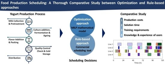
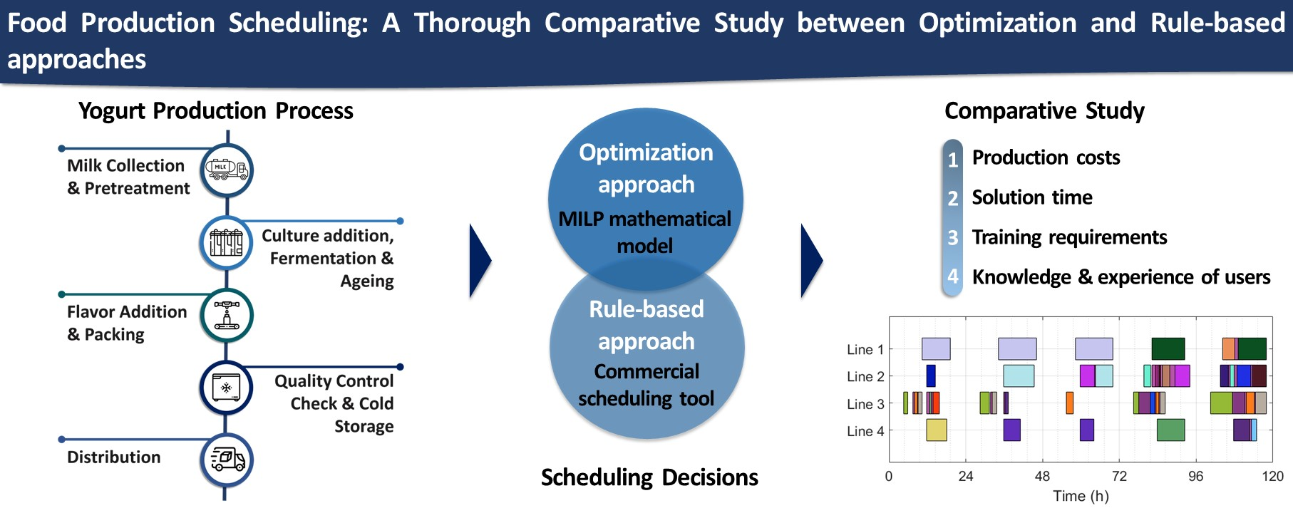
This work focuses on the production scheduling problem of multi-stage and multi-product industrial food processes and specifically on the semi-continuous yogurt production process of two large-scale Greek dairy industries. In this study, both optimization and rule-based approaches were utilized to generate production schedules for the continuous packing stage, which is identified as the bottleneck of the process. In order to solve the problem, two approaches were compared: (i) a precedence-based Mixed-Integer Linear Programming (MILP) model [18] and (ii) an interactive user-friendly commercial tool. Both approaches take into account all process-related constraints, including constraints of production stages that are not that explicitly modeled. Numerous real-life case studies were examined to assess the applicability and efficiency of the proposed solution frameworks. The main contribution of this work is to present for the first time a thorough evaluation and comparison of the applicability and performance of both optimization and rule-based approaches when applied to large real-life food scheduling problems. After a practical analysis is carried out upon real case studies, the advantages and disadvantages of the two approaches are detected, based on both qualitative and quantitative criteria, and significant insights are gained about the applicability of each method. Moreover, this research serves as a resource for practitioners in the field, providing valuable guidance for selecting the most suitable approach for scheduling problems in food industries.

This work is structured as follows: In Section 2, a detailed description of the process under consideration is provided, and the scheduling problems under study are outlined. Section 3 outlines the proposed modeling and solution strategies. Section 4 presents comparative results of the two strategies when applying to large-scale industrial cases. Finally, in Section 5, concluding remarks are drawn.

2. Problem Statement

Dairy industries are considered to be amongst the most dynamic food industries in the world. One of the most important products in the Greek dairy industry is yogurt. A plethora of yogurt types exist to satisfy the consumers’ individual needs and preferences. Yogurt products are classified into different categories based on various factors, including the type of milk used, the fat content, the production process, the flavor, the presence of probiotics and the level of sweetness [18]. Based on the milk source, yogurts can use cow’s milk, goat’s milk, sheep’s milk or other types of milk. Based on fat content, yogurts can be classified as whole, low-fat or non-fat. They can also be classified as sweetened with a specific sweetener or not and with or without added probiotics. Yogurt can also be flavored with fruit, spices or other ingredients. The aforementioned factors affect the calorie content of the product, its texture and its overall nutritional value.

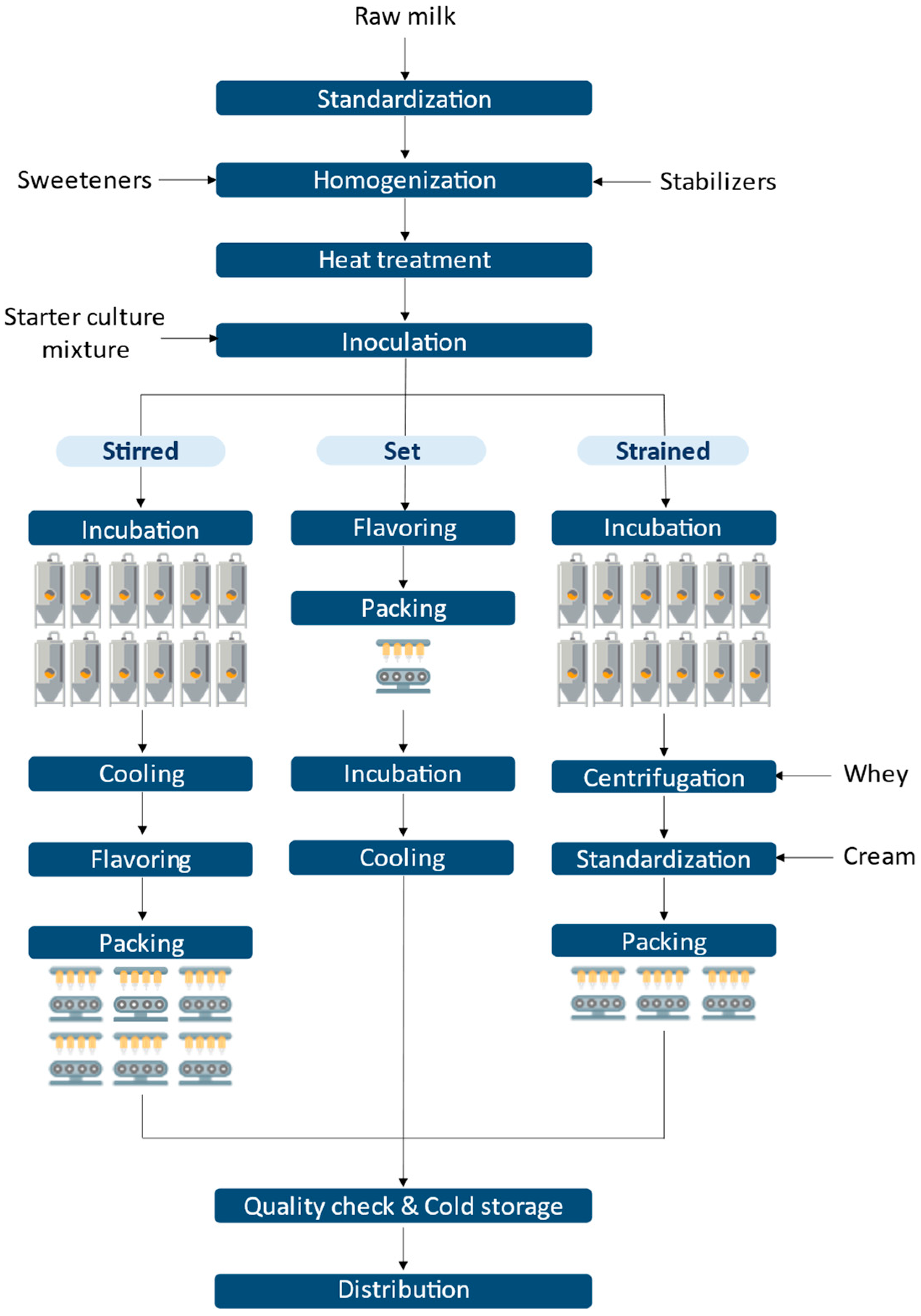
The most important classification of yogurt products is based on the production method used. There are two yogurt types based on this criterion: set and stirred yogurt. To produce set yogurt, the heated milk and culture mixture is poured into individual containers, such as plastic cups or glass jars, and it is left to ferment and form a solid, consistent product. On the other hand, to produce stirred yogurt, the milk and culture mixture is placed in a large tank and is continuously stirred for 2 to 4 h while it ferments and reaches the desired consistency. There are also some other types such as Greek yogurt, kefir and frozen yogurt.

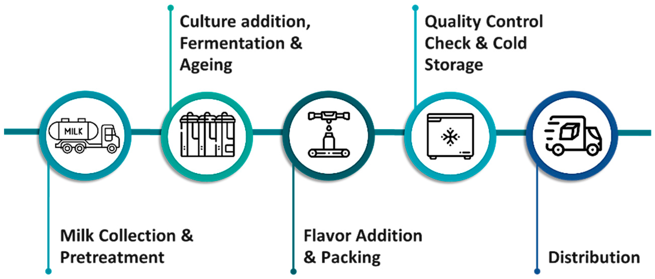
Slight modifications of the main production process are employed to produce each different type of yogurt. The main production process of yogurt products relies on the following stages:

• Milk Collection and Pretreatment
  Daily milk is collected from local farms, decontaminated and transferred to the factory. It should be noted that the composition of fresh milk in water, fat, protein, lactose and minerals varies from day to day. Once the milk reaches the factory, it is subject to a variety of processes including standardization, homogenization and heat treatment. Firstly, two types of standardization are implemented to improve the quality of the final yogurt product concerning the fat content and other non-fat-content-solids. Fat content is adjusted to meet compositional standards through the removal, mixing or addition of fat, while solids content is adjusted through the addition of milk powder, stabilizers, emulsifiers and other substances, such as sweeteners and preservatives. These adjustments are subject to specific legislative regulations. After being standardized, milk is homogenized so as to obtain a less creamy effect and to prevent clumping, leading to an improved appearance, texture and viscosity. Then, the milk is briefly heated to kill off pathogens.

• Culture Addition, Fermentation and Aging
  Lactic acid bacteria are added to the milk by mixing a pre-prepared culture of Streptococcus thermophilus and Lactobacillus bulgaricus into the milk. In some cases, other bacteria may be added to the culture to produce a specific type of yogurt. The milk and culture mixture is then placed in an incubation tank and maintained at the proper temperature for several hours. During this time, the bacteria ferment the lactose in the milk, producing lactic acid and thickening the milk into yogurt. The exact incubation time will vary depending on the temperature, the bacteria concentration, the type of yogurt being produced and the desired flavor and texture. Once the yogurt has thickened, it is cooled to 4 °C or lower to slow the growth of the bacteria and to stabilize the yogurt. The cooled yogurt is then stored for several hours. As mentioned before, set yogurt is fermented after packing, unlike other yogurt varieties.

• Flavor Addition and Packing
  Flavorings, such as syrups or fruit pieces, can be added to the yogurt after it has been thickened and cooled using a mixer. This allows a more distinct layering of flavors and a better texture. Some flavorings can also be added to the milk and culture mixture before it is incubated to integrate with the yogurt mixture. Finally, the yogurt is packed in a variety of containers, including plastic cups, glass jars, or larger containers. This is completed using parallel packing lines that can handle different types of yogurt products and packing options. During the packing process, the containers are filled with the desired yogurt, sealed and labeled with the product information required by law.

• Quality Control Check and Cold Storage
  Before reaching the consumers, the yogurt must pass a series of quality control checks to ensure that it meets quality standards, such as proper consistency, flavor and appearance. The packaged yogurt is then stored in a temperature-controlled environment, below 10 °C (usually between 2 °C and 8 °C), to maintain its quality until it is distributed to customers. This environment is typically a storage room or warehouse that is specifically designed for the storage of dairy products.

• Distribution to Customers
  The yogurt is finally transported to retail stores or distribution centers, where it is made available for sale to consumers. Customers are either directly served by the company’s refrigerated trucks, or they use their own transportation methods.

A brief schematic description of the aforementioned yogurt production process is shown in Figure 1.

The process under consideration is classified as multi-stage and multi-product, involving both batch and continuous stages.

The first problem examined concerns the production scheduling of the KRI-KRI dairy industry, which has been studied in our previous work [15]. The factory operates five to seven days a week and produces three types of yogurts (set, stirred, flavored), resulting in 93 final products that originate from 12 different recipes. Detailed information regarding the fermentation recipes is provided in

Table 1. Fermentation recipes data for the KRI-KRI facility.

Recipe	Fermentation Time (h)	Min Quantity (kg)	Cost (€)
R1	4.75	1200	545
R2	4.5	1200	540
R3	8.25	1200	565
R4	7.75	1200	555
R5	5.25	1200	525
R6	7.25	1200	565
R7	8.75	1200	625
R8	1.5	0	505
R9	1.5	0	510
R10	1.5	0	515
R11	8.75	1200	625
R12	8.75	1200	600

, and information regarding each product can be found in Table S2 of the supplementary material. Four packing lines are available, operating in parallel and sharing common resources. Each is responsible for the packing of specific products and has a minimum lot processing time of 0.5 h. It is noted that the factory does not operate on a 24 h basis but requires 3 and 2 h at the start and end of the day, respectively, for cleaning and maintenance processes. No production process takes place during these time frames. A families relative production sequence has been suggested by the company to facilitate production scheduling and reduce changeover costs.

The second problem concerns the production scheduling of the dairy industry TYRAS, which is a member of the Hellenic Dairy S.A. Group. The production steps of this plant are illustrated in Figure 2. The plant operates seven days a week and produces three main types of yogurt (strained, directly set, cohesive stirred), resulting in 176 final products derived from 16 different recipes. More information concerning the fermentation recipes is available in

Table 2. Fermentation recipes data for the TYRAS facility.

Recipe	Fermentation Time (h)	Min Quantity (kg)	Max Quantity (kg)
R1	8.50	3500	52,222
R2	7.50	3500	52,222
R3	7.50	3500	52,222
R4	6.00	3500	52,222
R5	6.50	3500	36,000
R6	1.00	3500	30,000
R7	7.50	3500	52,222
R8	8.50	3500	36,000
R9	8.50	3500	36,000
R10	13.50	3500	36,000
R11	7.50	3500	52,222
R12	1.00	3500	30,000
R13	8.50	3500	36,000
R14	8.50	3500	36,000
R15	1.00	3500	30,000
R16	1.00	3500	30,000

, and information regarding each product is available in Table S7 of the supplementary material. This plant has a more complicated packing stage including seven parallel packing lines. The plant operates on a 24 h basis; however, every packing line requires a few hours at the end of the day for cleaning and maintenance processes (see

Table 3. Packing lines data for the TYRAS facility.

Line	Setup Time (h)	Shutdown Time (h)	Available Production Time (h)
J1	0.13	1.33	22.54
J2	0.13	1.33	22.54
J3	0.13	1.50	22.37
J4	0.13	1.67	22.20
J5	0.13	1.67	22.20
J6	0.13	1.67	22.20
J7	0.13	1.67	22.20

). During this time, no packing process can be carried out on any line; however, the fermentation processes can still be performed, since they are carried out on different units.

The main production characteristics of each industrial plant are summarized in

Table 4. Main production characteristics.

	(A) KRI-KRI	(B) TYRAS
Products	93	176
Recipes	12	16
Families	23	41
Fermentation tanks	15	12
Packing lines	4	7
Scheduling horizon in days	5	7

.

The scheduling problem is focused on the continuous packing stage, as this represents the main production bottleneck in both facilities. However, previous production stages are modeled as an equivalent stage of a certain known duration, independent of the batch size, which, nevertheless, respects all the underlying operating constraints and ensures schedule feasibility throughout the whole plant.

Due to the large number of products, the problem may become quite complex to be solved using optimization techniques. For this reason, products with similar characteristics are treated as a group that is referred to as a product family, thus resulting in a simpler problem with lower computational requirement. The idea of product families leads to equivalent solutions with the ones derived by using the whole set of products. Products of a single family necessarily come from the same recipe, require the same resources, and do not necessitate changeover actions during sequential production [15]. Conversely, for the sequential production of two products belonging to different families, it is necessary to include cleaning and sterilization processes in the packing line. It is important to note that while products from the same family share many common features, they can still present differences in terms of processing rate, capacity, timing and costs.

The main scheduling challenges for the problem under consideration are associated with allocation, sequencing and timing constraints. There are numerous fermentation tanks for the preparation of yogurt, and each one can feed more than one packing line, thus providing flexibility to the production process. Intermediate storage vessels are not necessary, since the yogurt mixture can be temporarily stored in the fermentation tanks for up to 24 h. However, each packing line can only process specific final products, one at a time, thus limiting the flexibility provided by the tanks. Moreover, the packing lines must be cleaned in between the processing of two different product families; thus, a sequence-dependent changeover time is necessary (see Tables S5 and S9 of the supplementary material). Sequence independent setup times for adjusting machines’ settings also take place before the packing of each product family. The main goal is the efficient scheduling of these facilities, given a weekly product demand.

The problem under study can be formally defined as follows:

Given:

• The planning horizon of interest divided into a set of time periods.
• A set of parallel packing lines and their available production time in each period.
• A set of batch recipes with minimum preparation time and specified production capacity.
• A set of products.
• A set of product families in which all products are grouped.
• Assignment suitability constraints between packing lines, products, recipes and product families.
• All production-related parameters including production targets, production rates, minimum and maximum processing runs, cup weights, daily opening and shutdown times.
• The required sequence-dependent changeover operations whenever a new family is processed after a previous one in each processing unit, as long as the processing sequence is not forbidden.
• The required sequence-independent setup operations whenever a product is assigned to a processing unit.
• The cost coefficients associated with recipes preparation, unit operation, changeovers, inventory and external production.

Determine:

• The assignment of product families to packing lines.
• The sequencing of product families in each packing line.
• The amount of every product produced in each processing unit.
• The production run length, starting and completion time for every product family.
• The amount of every product externally produced in a cooperating plant.
• The inventory level for every product in each time period.

Thus, an objective function typically representing total production costs is optimized.

It is noted that the availability of raw materials is assumed to be constant, and limitations such as manpower or utilities are not considered. The transfer of yogurt liquid between the two stages is assumed to take place instantaneously, and the fermentation/maturation process in a tank only begins at the start of each time period. Production data are assumed to be deterministic, and the incorporation of uncertainty is beyond the scope of this work.

3. Materials and Methods

3.1. MILP Model

An MILP model was applied to efficiently address the production lot-sizing and scheduling problem for a dairy multi-stage and multi-product facility [18]. The model includes mass balance, assignment, timing and sequencing constraints. The model relies on a novel mixed discrete-continuous time representation, where the production horizon is divided in distinct time periods with the duration of a day. Detailed timing decisions and process representation within each period are modeled in a continuous manner. Scheduling decisions are made based on the concept of product families instead of single products, thus facilitating the problem solution.

A brief description of the constraints comprising the applied mathematical model and what they establish is presented below. The detailed description of the model is available in our previous works [15,18].

$${\pi }_{p,j,n}^{min}·{\overline{{\rm Y}}}_{p,j,n}\le Q_{p,j,n}\le {\pi }_{p,j,n}^{max}·{\overline{{\rm Y}}}_{p,j,n}\forall p,j\in J_P,n$$

(1)

$${{\rm Y}}_{f,j,n}\ge {\overline{{\rm Y}}}_{p,j,n}\forall f,p\in Pf,j\in J_f,n$$

(2)

$$V_{j,n}\ge Y_{f,j,n}\forall f,j\in J_f,n$$

(3)

$${\displaystyle \sum }_{f^{\prime }\ne f,f^{\prime }\in Fj}{{\rm X}}_{f^{\prime },f,j,n}\le Y_{f,j,n}\forall f,j\in J_f,n$$

(4)

$${\displaystyle \sum }_{f^{\prime }\ne f,f^{\prime }\in Fj}{{\rm X}}_{f,f^{\prime },j,n}\le Y_{f,j,n}\forall f,j\in J_f,n$$

(5)

$${\displaystyle \sum }_{f\in Fj}{\displaystyle \sum }_{f^{\prime }\ne f,f^{\prime }\in Fj}{{\rm X}}_{f,f^{\prime },j,n}+V_{j,n}={\displaystyle \sum }_{f\in Fj}{Y}_{f,j,n}\forall j,n$$

(6)

$$C_{f,j,n}+{\gamma }_{f,f^{\prime },j}.{{\rm X}}_{f,f^{\prime },j,n}\le S_{f^{\prime },j,n}+{{\rm M}}_{j,n}\left(1-{{\rm X}}_{f,f^{\prime },j,n}\right)\forall f,f^{\prime },j\in \left(J_f{\displaystyle \cap }{J}_{f^{\prime }}\right),n$$

(7)

$$T_{f,j,n}={\sum }_{p\in Pf}(\frac{Q_{p,j,n}}{{\rho }_{p,j}}+{\delta }_{p,j}·{\overline{{\rm Y}}}_{p,j,n})\forall f,j\in J_f,n$$

(8)

$$S_{f,j,n}=C_{f,j,n}-{{\rm T}}_{f,j,n}\forall f,j\in J_f,n$$

(9)

$$C_{f,j,n}\ge (a_{j,n}+{\tau }_r)·Y_{f,j,n}+T_{f,j,n}+{\displaystyle \sum }_{f^{\prime }\ne f,f^{\prime }\in Fj}{\gamma }_{f^{\prime },f,j}{{\rm X}}_{f^{\prime },f,j,n}\forall f,r\in R_{f,}j\in J_f,n$$

(10)

$$C_{f,j,n}\le ({\omega }_{j,n-}{\beta }_{j,n})·Y_{f,j,n}\forall f,j\in J_f,n$$

(11)

$${\mu }_{r,n}^{min}·Y_{r,n}^R\le {\displaystyle \sum }_{p\in P_r}{\displaystyle \sum }_{j\in J_p}{Q}_{p,j,n}\le {\mu }_{r,n}^{m\alpha x}·Y_{r,n}^R\forall r,n$$

(12)

$$Y_{r,n}^R\ge {\displaystyle \sum }_{j\in J_f}{Y}_{f,j,n}\forall r,f\in F_r,n$$

(13)

$$Q_{p,n}^{int}={\displaystyle \sum }_{j\in J_P}{Q}_{p,j,n}\forall p,n$$

(14)

$$I_{p,n}=I_{p,n-1}+Q_{p,n}^{int}+Q_{p,n}^{ext}-{\zeta }_{p,n}\forall p,n$$

(15)

$$Q_{p,n}^{ext}\le {\zeta }_{p,n}\forall p,n$$

(16)

$$\begin{array}{c}min{\displaystyle {\displaystyle \sum }_p}{\displaystyle {\displaystyle \sum }_n}{\xi }_{p,n}·I_{p,n}+{\displaystyle {\displaystyle \sum }_p}{\displaystyle {\displaystyle \sum }_{j\in J_p}}{\displaystyle {\displaystyle \sum }_n}\frac{{\theta }_{p,j,n}}{{\rho }_{p,j}}·Q_{p,j,n}+{\displaystyle {\displaystyle \sum }_r}{\displaystyle {\displaystyle \sum }_n}{\chi }_{r,n}·Y_{r,n}^R+{\displaystyle {\displaystyle \sum }_j}{\displaystyle {\displaystyle \sum }_n}{\nu }_{j,n}·V_{j,n}\\ +{\displaystyle {\displaystyle \sum }_f}{\displaystyle {\displaystyle \sum }_{f^{\prime }\ne f}}{\displaystyle {\displaystyle \sum }_{j\in (J_f{\displaystyle \cap }{J}_{f^{\prime }})}}{\displaystyle {\displaystyle \sum }_n}{\phi }_{f,f^{\prime },j,n}·{{\rm X}}_{f,f^{\prime },j,n}+{\displaystyle {\displaystyle \sum }_p}{\displaystyle {\displaystyle \sum }_n}{\psi }_{p,n}·Q_{p,n}^{ext}\end{array}$$

(17)

Products Lot-Sizing Constraints

• Constraint (1) imposes lower, ${\pi }_{p,j,n}^{min}$, and upper, ${\pi }_{p,j,n}^{max}$, bounds on the produced amount of product p in processing unit j and in time period n, $Q_{p,j,n}$, if that product is to be produced (${\overline{{\rm Y}}}_{p,j,n}$ = 1). The upper bound is either equal to the remaining demand until the end of the scheduling horizon or to the maximum amount of product that can be processed by the packing line in the current time period.

Families Allocation Constraints

• Constraint (2) ensures that if at least one product p that belongs to a specific family f is processed on unit j in time period n, then this family will be assigned to this unit in the same time period (${{\rm Y}}_{f,j,n}$ = 1).
• Constraint (3) ensures that a packing line is used in a time period ($V_{j,n}$ = 1) if at least one family is assigned to it for that particular time period.

Families Sequencing Constraints

• Constraints (4) and (5), utilizing the sequence binary variable ${{\rm X}}_{f,f^{\prime },j,n}$, establish that if a family is assigned to a specific processing unit during a time period, then this family has at most one predecessor and one successor.
• Constraint (6) imposes that the sum of the total active sequence binary variables ${{\rm X}}_{f^{\prime },f,j,n}$ and the binary variable $V_{j,n}$, which indicates whether a packing line is used, must equal the total number of active allocation variables in the packing line ${{\rm Y}}_{f,j,n}$ in each time period. For example, if three families are produced in a packing line, then there are three active allocation variables, two active sequence binary variables and an active binary line utilization variable, as shown in Figure 3.

Families Timing Constraints

• Constraint (7) states that the starting time of processing a product family f′, $S_{f^{\prime },j,n}$, after another family f in a unit j, is greater than the sum of the completion time of the first family, $C_{f,j,n}$, and the necessary changeover time between the families ${\gamma }_{f,f^{\prime },j}$. This is a big M-constraint, meaning that in case a families sequence is not selected, the starting time of family f′ must be greater than a very small number. ${{\rm M}}_{j,n}$ represents the available processing time minus the daily shutdown time for packing line j in time period n.
• Constraints (8) and (9) define a family’s processing time, $T_{f,j,n},$ as the total processing time for all products that belong to the family, which is calculated as the produced amount of products divided by their production rate, ${\rho }_{p,j}$, plus the required set up times, ${\delta }_{p,j},$ in order to process each product.
• Constraints (10) and (11) introduce lower and upper bounds in the families completion times. More specifically, the completion time of a family must be greater than the sum of the daily plant startup time, $a_{j,n}$, the minimum time for the fermentation recipe preparation, ${\tau }_r$, the family processing time and the necessary changeover time. Additionally, the completion time of a family must not exceed the available daily production horizon, ${\omega }_{j,n}$, minus the daily shutdown time of the plant, ${\beta }_{j,n}$.

Recipe Preparation Batch Stage Constraints

• Constraint (12) bounds the total produced quantity of products between the minimum produced recipe amount, ${\mu }_{r,n}^{min}$, and the maximum recipe production capacity, ${\mu }_{r,n}^{m\alpha x}$, if recipe r which produces product p is used in period n ($Y_{r,n}^R$ = 1).
• Constraint (13) guarantees that a recipe is produced in a time period if at least one family deriving from this recipe is processed in a packing line in the same time period.

Mass Balance Constraints

• Constraints (14)–(16) ensure full demand satisfaction, under the expression that the inventory of a product at the end of a time period, $I_{p,n}$, equals the previous time period inventory, $I_{p,n-1}$, plus the total internal, $Q_{p,n}^{int}$, and external production, $Q_{p,n}^{ext}$, minus the production targets of the time period, ${\zeta }_{p,n}$. The external production term demonstrates production realized to an affiliated production facility or the unsatisfied demand and in no case should exceed the current period’s demand.

Objective Function

• The objective of the mathematical model (17) is the minimization of the total production cost, which includes costs of storage, ${\xi }_{p,n}$, internal production, ${\theta }_{p,j,n}$, recipe preparation, ${\chi }_{r,n}$, packing line utilization, ${\nu }_{j,n}$, families changeovers, ${\phi }_{f,f^{\prime },j,n}$, and external production, ${\psi }_{p,n}$.

The implementation of the described MILP mathematical model is realized using the GAMS optimization tool [35].

3.2. Commercial Scheduling Tool (SchedulePro^TM)

Most of the food process industries, such as the dairy industries, are strictly structured and organized with limited flexibility. Α recipe-based approach was chosen to represent the production process of the two dairy plants. The entire process is broken down into recipes or formulas, which can be easily replicated to create consistent production. More specifically, the recipe-based, finite capacity, scheduling tool of Intelligen Inc. (Scotch Plains, NJ, USA), SchedulePro^TM [33], is deployed to set up and solve the scheduling problems. This tool is chosen because of its rich representation language, computational speed and interactive scheduling logic.

SchedulePro^TM functions as a modeling and simulation-based production planning and scheduling tool. It offers a rich representation language and an interactive scheduling logic, which enables the handling of complex scheduling problems [32,33]. It is a recipe-driven tool that generates feasible solutions satisfying major constraints but does not guarantee solution optimality. The produced feasible and acceptable schedules can be further improved interactively by the user, using intuitive interfaces that enable visualization and easy modification of the schedule [36]. This tool facilitates design, debottlenecking, capacity analysis, improvement of equipment utilization and quick rescheduling of multi-product facilities that operate in batch or semi-continuous mode. By combining the expertise and knowledge of both the user and the scheduling software, a more realistic and effective production plan can be created that meets the production objectives in a timely and efficient manner.

A typical process of describing a scheduling problem into the SchedulePro^TM software includes the following steps [33]:

• Declaration of recipes: Recipes contain information about the processing steps required to produce the final product. They consist of procedures which include operations that consume resources and produce the desired materials. Each procedure has its own equipment pool (processing units) where it can take place, while operations may also have auxiliary equipment or resources. The duration of each operation as well as its timing with respect to other tasks is declared. Whether the operation is interruptible or delayable should also be stated. This step also involves defining the standard recipe for each product to be manufactured.
• Declaration of available equipment and resources: This involves identifying the available equipment, labor, storage, utilities, etc. and the production capacity of each resource. Parallel use of equipment or resources and possible existing downtimes are also declared.
• Declaration of production campaigns: This involves creating a campaign of recipes that define the batches that need to be produced. A release or due date for each campaign can be stated.
• Schedule generation and modification: A production schedule that indicates when each batch will be produced, which resources will be used and how long each step of the process will take is automatically generated. The generated schedule can be inspected by the users through various tables and graphs, such as economic reports or the equipment occupancy chart, which helps to identify potential bottlenecks or scheduling conflicts. Moreover, resource graphs are also available to capture the consumption and inventory of resources such as materials and utilities against their availability. The generated schedule can be modified as needed to accommodate changes in production requirements, resource availability or other factors. Tracking the status of production as a function of time is possible; thus, well-informed and timely decisions can be easily made to ensure that production objectives are met.

SchedulePro^TM allows the user to insert the production process in great detail, thus creating a digital twin. The problem considered in this work is implemented in SchedulePro^TM in the following sequence.

• First, the production facility and the scheduling horizon are identified, and then, potential existing downtimes are declared. These downtimes can refer to weekends, plant setup and shutdown times, scheduled maintenance, etc.
• All products in the plant are declared in the SKUs table. Two SKU types are inserted: one containing the product families and one containing the fermentation recipes/formulas. The mapping between SKUs and types is also realized.
• The available equipment of the facility and its possible outages are added. The minimum and maximum capacity of fermentation tanks as well as which fermentation recipes they can produce are defined. For the packing lines, a setup time and a product-dependent rate is set. Moreover, a changeover matrix is inserted including the changeover time needed by each specific equipment for the sequential processing of two product families.
• Regarding the introduction of the production process, a single semi-continuous recipe is declared for all yogurt products. Note that this “recipe” refers to the production process and not to the fermentation recipes/formulas needed to prepare yogurts. This recipe consists of two procedures, one for the yogurt preparation stage and one for the packing stage. The main equipment responsible for the execution of each procedure is declared. The first procedure includes one operation, the actual fermentation process, and the second procedure is further divided into three operations: one for the product-dependent changeover, one for the machine setup time and one for the filling process. An SKU-type-specific fixed duration is set for the fermentation operation, which is scheduled as the first operation to take place. The duration of changeover operations is set based on the equipment changeover times declared with respect to the task before. This operation is scheduled to start with the end of the fermentation operation, and a flexible time shift is added regarding the equipment availability. The duration of the setup operation is set equal to the equipment’s setup time, and the operation is scheduled to start after the end of the changeover operation. Finally, the duration of the filling operation is set as rate-based, and it is equipment dependent and scalable with batch size. This operation is scheduled right after the setup operation. The operation responsible for producing the final products is defined as the filling operation.
• To fulfill the facility’s pending orders, campaign projects are created for each day of the week. A campaign can be based on an SKU order template and specifies how many batches of each product need to be produced and within which time frame. It is noted that the order in which the campaigns are inserted has a major impact on the derived schedule; therefore, extensive knowledge of the facility is required to obtain acceptable and near-optimal schedules.

The scheduling algorithm of SchedulePro^TM takes into consideration the campaign’s priority in order to achieve makespan minimization. Proper start times using the earliest available resources to avoid arising conflicts are defined. It should be emphasized that SchedulePro^TM is not an optimization tool but rather a simulation scheduling tool that allows the integrated description and management of production facilities using simple rule-based approaches. Eventually, a feasible production schedule is extracted, and after potential modifications to accommodate production requirements, it can be visualized through various reports, including tables and graphs. These reports provide important information regarding assignment, timing, equipment utilization, production costs, inventory tracking and much more, which can be used for timely and efficient decision making by the production engineers.

4. Results and Discussion

In this section, various case studies are examined to evaluate the efficiency and applicability of the proposed methods to real-life problem instances. More specifically, the production scheduling of each facility is derived given a weekly demand (see Tables S3 and S8 of the supplementary material), and a comparative study between the two methods is conducted. Additional case studies concerning the capacity expansion of specific lines are also considered. A detailed description of the case studies under consideration is provided in

Table 5. Case studies description.

Case	Details
A1	Basic scenario for KRI-KRI facility
A1.1	A1 solved using a random sequence of production orders in ScheduleProTM
A1.2	A1 solved using the given families relative sequence of production in ScheduleProTM
A1.3	A1 solved using an experience-based sequence of production orders in ScheduleProTM
A1.4	A1 solved using the MILP model
A2	Addition of an extra packing line identical to line 1 in KRI-KRI facility
A2.1	A2 solved using a random sequence of production orders in ScheduleProTM
A2.2	A2 solved using the given families relative sequence of production in ScheduleProTM
A2.3	A2 solved using an experience-based sequence of production orders in ScheduleProTM
A2.4	A2 solved using the MILP model
A3	Addition of an extra packing line identical to line 2 in KRI-KRI facility
A3.1	A3 solved using a random sequence of production orders in ScheduleProTM
A3.2	A3 solved using the given families relative sequence of production in ScheduleProTM
A3.3	A3 solved using an experience-based sequence of production orders in ScheduleProTM
A3.4	A3 solved using the MILP model
B1	Basic scenario for TYRAS facility
B1.1	B1 solved using a random sequence of production orders in ScheduleProTM
B1.2	B1 solved using an experience-based sequence of production orders in ScheduleProTM
B1.3	B1 solved using the MILP model
B2	Addition of an extra packing line identical to line 2 in TYRAS facility
B2.1	B2 solved using a random sequence of production orders in ScheduleProTM
B2.2	B2 solved using an experience-based sequence of production orders in ScheduleProTM
B2.3	B2 solved using the MILP model

.

As mentioned before, the quality of the results using SchedulePro^TM depends on the user’s knowledge of the facility and experience with the software. Therefore, case studies which cover different insertion sequencing policies of the production targets are considered. No matter the level of knowledge of the production process or experience of the plant engineers and operators, it is still impossible to reach nearly optimal results for highly combinatorial problems without employing formal optimization methods. Regarding the MILP-based optimization approach, the model is implemented in GAMS 41.5.0 and solved using CPLEX 12.0 in a PC equipped with an Intel Core i5 @2.9 GHz CPU and 16 GB of RAM.

Table 6. Families production relative sequence concerning cases of the KRI-KRI facility.

Line	Families Relative Sequence
J1	F20 →	F21 →	F22
J2	F12 →	F11 →	F19 →	F18 →	F13 →	F14 →	F15 →	F16 →	F17
J3	F01 →	F02 →	F03 →	F05 →	F04 →	F08 →	F09 →	F10 →	F06 →	F07
J4	F08 →	F09 →	F10 →	F06 →	F23

illustrates the families production relative sequence suggested by the company and used for cases A1.2, A2.2, A3.2. Τhe direction of the arrows helps to indicate that the production progresses from one product family to the next following the specified order.

Table 7. Comparison between the MILP model and the proposed rule-based approach of SchedulePro^TM for cases of the KRI-KRI facility.

	Case	Production Cost (€)	Improvement (%)	Weekly Makespan (h)	Avg Daily Makespan (h)	Cmax (h)	CPU (s)
A1	A1.1	808,094	-	117.28	21.67	21.90	1.32
	A1.2	450,206	44.3	116.62	21.41	21.95	1.08
	A1.3	381,223	52.8	116.62	21.41	21.95	1.04
	A1.4	317,852	60.7	118.00	21.44	22.00	1.87
A2	A2.1	569,604	-	117.28	21.27	21.85	1.13
	A2.2	393,266	31.0	116.47	21.08	21.95	1.07
	A2.3	339,213	40.4	116.47	20.60	21.95	1.10
	A2.4	274,961	51.7	118.00	21.10	22.00	2.06
A3	A3.1	584,415	-	115.78	21.37	21.89	1.19
	A3.2	331,795	43.2	116.62	21.13	21.82	1.02
	A3.3	292,084	50.0	116.62	21.13	21.82	1.07
	A3.4	263,951	54.8	118.00	21.22	22.00	1.97

summarizes the solution characteristics of all cases for the KRI-KRI facility. A comparison between the two computational approaches for each main problem (e.g., A1, A2, A3) is presented based on the solution time, production cost and makespan of the generated schedules. It is observed that both SchedulePro^TM and the optimization model generate solutions instantaneously for problems of this complexity. In terms of the production cost, the MILP model leads to much better solutions compared to SchedulePro^TM.

It is clear that the deeper the knowledge and experience of the user, the better the obtained solution using SchedulePro^TM. For the case of little to no experience of the user (A*.1), meaning a random insertion sequence of the production targets, as the base case, the production cost seems to gradually decrease as the experience of the user increases (A*.1 → A*.2 → A*.3). An experienced user can create schedules up to 53% improved compared to a non-experienced user, while the MILP model leads to further improved solutions, up to 61%. 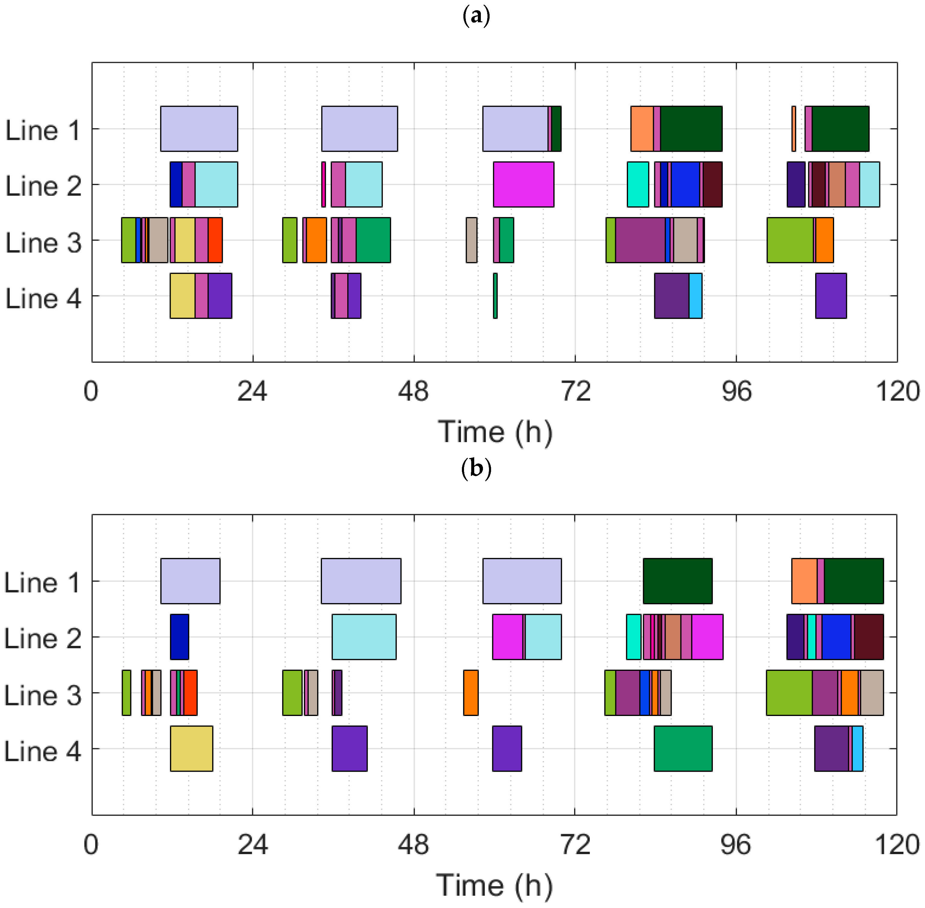The MILP model also compares favorably with the solutions generated by an experienced user of SchedulePro^TM. Part of the improvement in the experienced user cases is a result of the follow-up interactive modification of the proposed schedule. Through these case studies, it is validated that empirical rules, such as the relative production sequence of the product families, can significantly affect the quality of the obtained schedule. Nevertheless, the level of optimality of the solution cannot reach the corresponding one of the MILP model for complex industrial processes. As shown in the Gantt chart depicted in Figure 4, a non-experienced user of SchedulePro^TM will derive schedules in which product families are assigned to different packing lines and production days compared to the solution of the optimization approach, leading to increased production costs. Each uniquely colored rectangular represents the processing of a product family.

Although SchedulePro^TM is not an optimization software, it derives schedules with respect to makespan minimization by default. Table 7 indicates that the generated schedules lead to smaller daily and weekly makespans compared to the corresponding ones derived by the mathematical model. Nevertheless, the difference for the specific problem instances is not considered as significant.

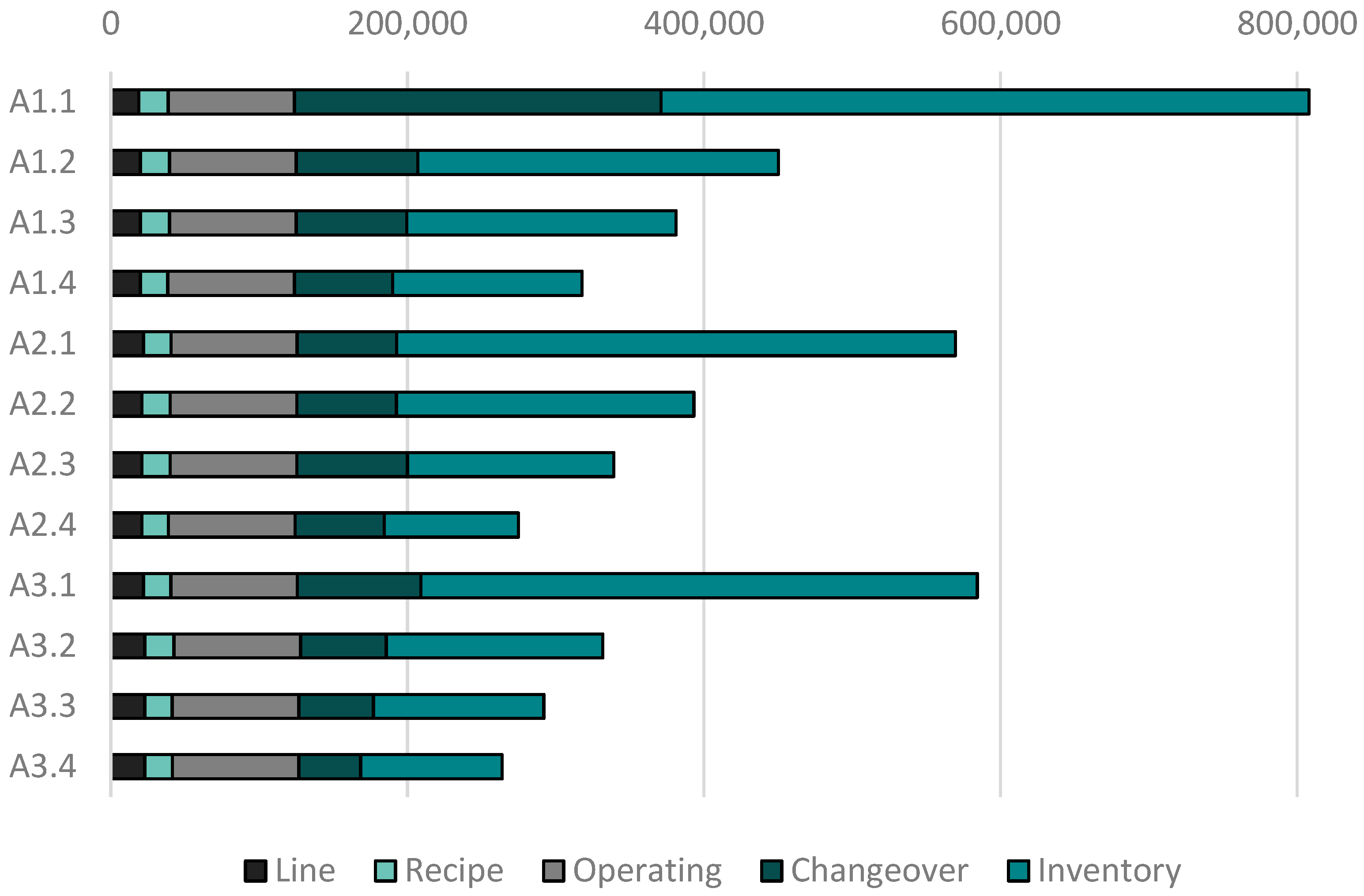
The total production cost consists of five elements and is calculated as shown in

Table 8. Total production cost breakdown for cases of the KRI-KRI facility.

Type of Cost	Amount
Line utilization	1000 €/line and day of operation
Recipe preparation	Recipe cost (Table 1)/recipe and day used
Operating	500 €/h of operation of line
Changeover	Changeover cost (Table S4)/type of changeover
Inventory	Inventory cost (Table S2)/kg of product stored
External production	30 €/kg of product produced externally

.

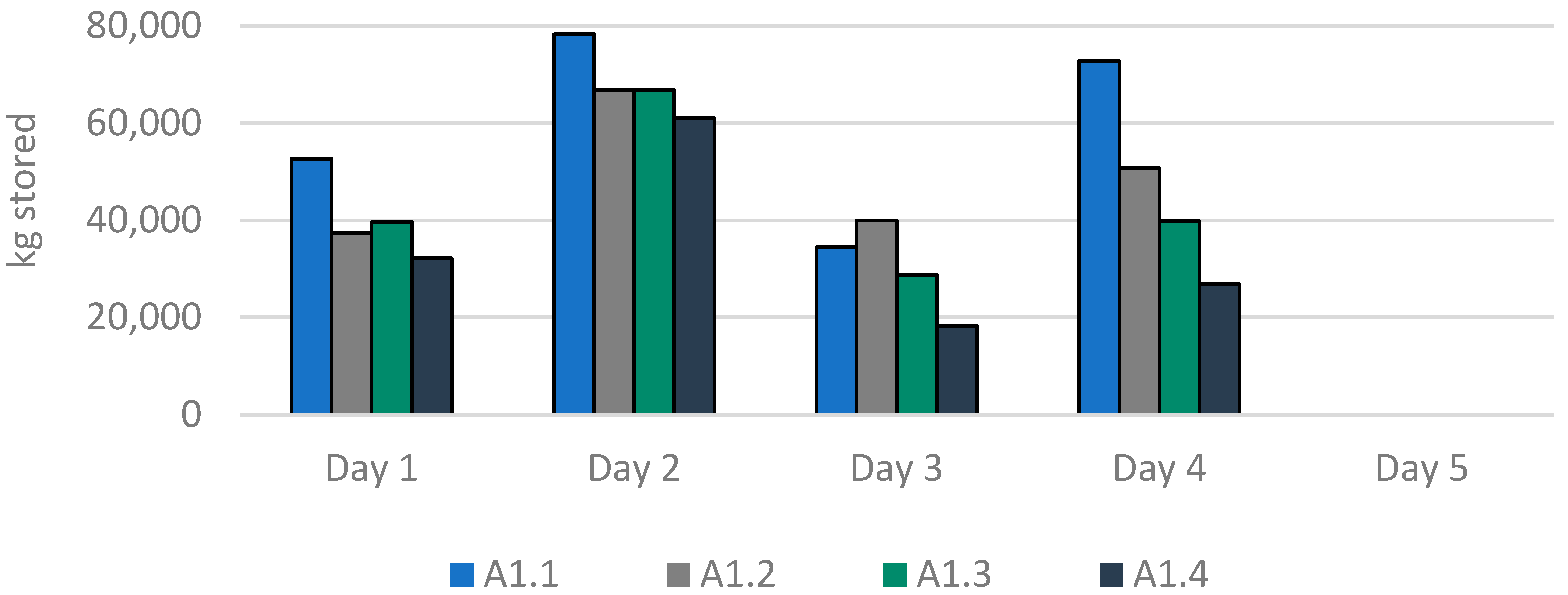
Based on Figure 5, inventory costs comprise the majority of the total production cost, which are followed by the operating and changeover costs. For the rule-based approach solutions, inventory and changeover costs define the size of the total cost and seem to vary depending on the user’s knowledge of the production process. Other cost items are similar to the ones defined by the MILP model. Neither approach presents external production costs. Each solution approach leads to different inventory profiles, thus resulting in different inventory costs. For problem A1, the case of the non-experienced user of SchedulePro^TM presents the highest volumes of stored products, while the case of the optimization approach presents the smallest, as shown in Figure 6. Moreover, the optimization approach is the only one which does not leave excess products in the warehouse at the end of the scheduling horizon.

Table 9. Production cost reduction due to capacity expansion of the KRI-KRI facility.

Initial Capacity	Extra Line Identical to Line 1		Extra Line Identical to Line 2
A1.1	(A2.1)	−29.5%	(A3.1)	−27.7%
A1.2	(A2.2)	−12.6%	(A3.2)	−26.3%
A1.3	(A2.3)	−11.0%	(A3.3)	−23.4%
A1.4	(A2.4)	−13.5%	(A3.4)	−17.0%

shows how each solution method handles the capacity expansion of the KRI-KRI facility in terms of production cost. It is observed that a capacity expansion results in production cost reduction in all cases, with the addition of an extra line identical to line 2 being the most beneficial option. The reduction in the total production cost is mainly due to reductions in changeover and inventory costs.

In a similar way,

Table 10. Comparison between the MILP model and the proposed rule-based approach for cases of the TYRAS facility.

	Case	Production Cost (€)	Improvement (%)	Weekly Makespan (h)	Avg Daily Makespan (h)	Cmax (h)	CPU (s)
B1	B1.1	-	Infeasible	-	-	-	-
	B1.2	812,646	-	165.30	21.17	22.60	0.87
	B1.3	715,075	12.0	165.97	21.60	22.67	144.29
B2	B2.1	-	Infeasible	-	-	-	-
	B2.2	805,625	-	164.72	21.12	22.47	0.87
	B2.3	713,112	11.5	165.72	20.95	22.67	269.61

presents the solution characteristics of all cases considered for the TYRAS facility. In this problem instance, the knowledge and experience of the user is a catalytic factor for the extraction of a feasible production schedule using SchedulePro^TM. It is noted that a completely random insertion sequence of the production targets, due to lack of experience or knowledge of the production process, leads to an infeasible production schedule which violates certain constraints. Long changeovers, emerging from the random sequence of product families production, lead to a failure of timely satisfaction of the weekly product demand. Only an experienced user can derive feasible and efficient schedules for a production process of this complexity using a rule-based approach. On the other hand, it is guaranteed that the MILP model will always derive an optimal solution for the same problem. In this case, optimally derived production schedules are compared favorably with the corresponding schedules of an experienced user using SchedulePro^TM. 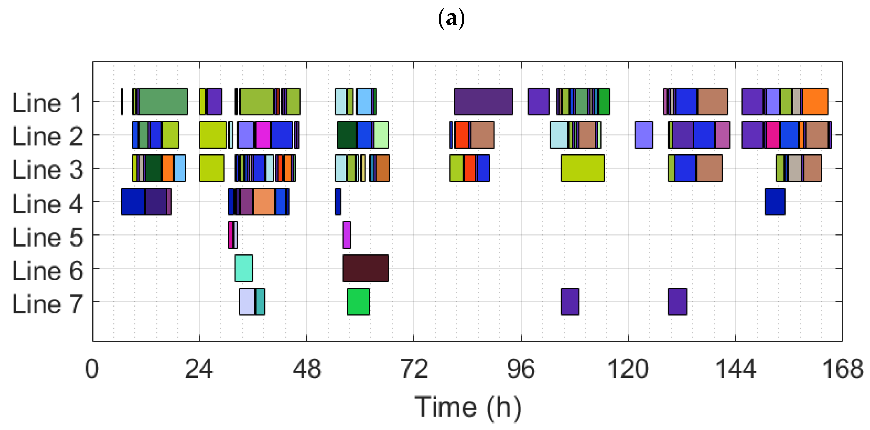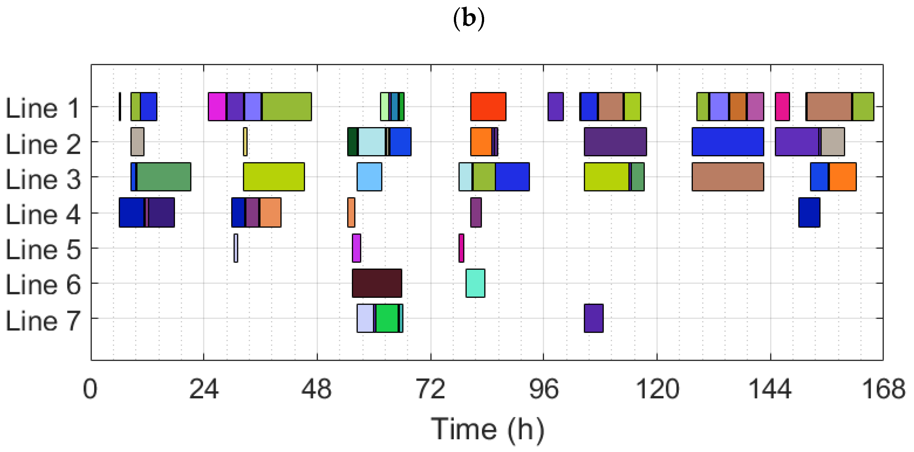Figure 7 illustrates the different production schedules a user can derive using SchedulePro^TM with prior experience and using the optimization approach. It is observed that SchedulePro^TM allocates product families differently and leads to larger production volumes compared to the optimization approach in order to respect all major constraints.

SchedulePro^TM generates results significantly faster than the MILP model. Nevertheless, both CPU times are acceptable by the industry in the context of weekly production scheduling. It is clear that the size of the problem seriously affects the CPU solution time for the optimization-based approaches, while the rule-based approaches are unaffected by this factor. This could be an issue for very large problem instances where the computation times of the MILP model might not be acceptable by the industry, especially in cases of a highly dynamic environment that requires frequent and fast rescheduling actions.

Moreover, the rule-based approach produces schedules characterized by smaller daily and weekly makespans than the ones derived by the optimization model. Nonetheless, the difference is not deemed as significant. This can be attributed to the fact that the goal of the MILP model is cost minimization, thus leading to decisions which reduce costs by sacrificing production makespan to a small extent.

The total production cost for this problem is calculated based on the costs shown in

Table 11. Total production cost breakdown for cases of the TYRAS facility.

Type of Cost	Amount
Line utilization	50 €/line and day of operation
Recipe preparation	-
Operating	2 €/kg of product produced
Changeover	1300 €/h of changeover
Inventory	0.1 €/kg of product stored and day
External production	-

.

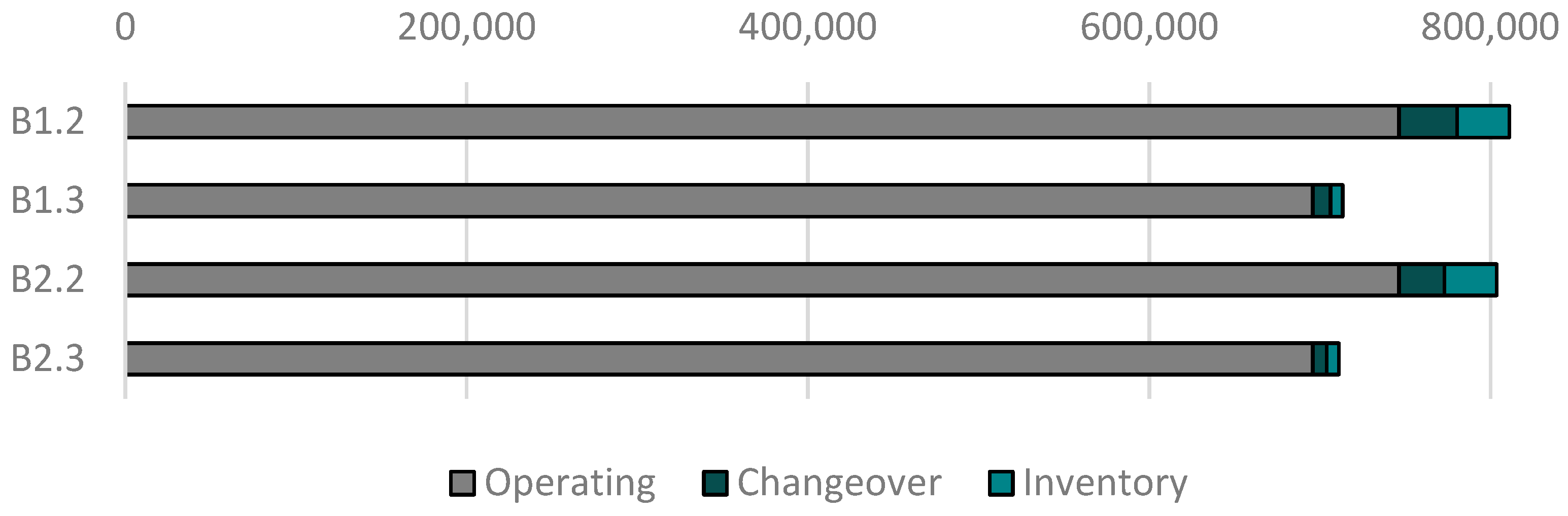
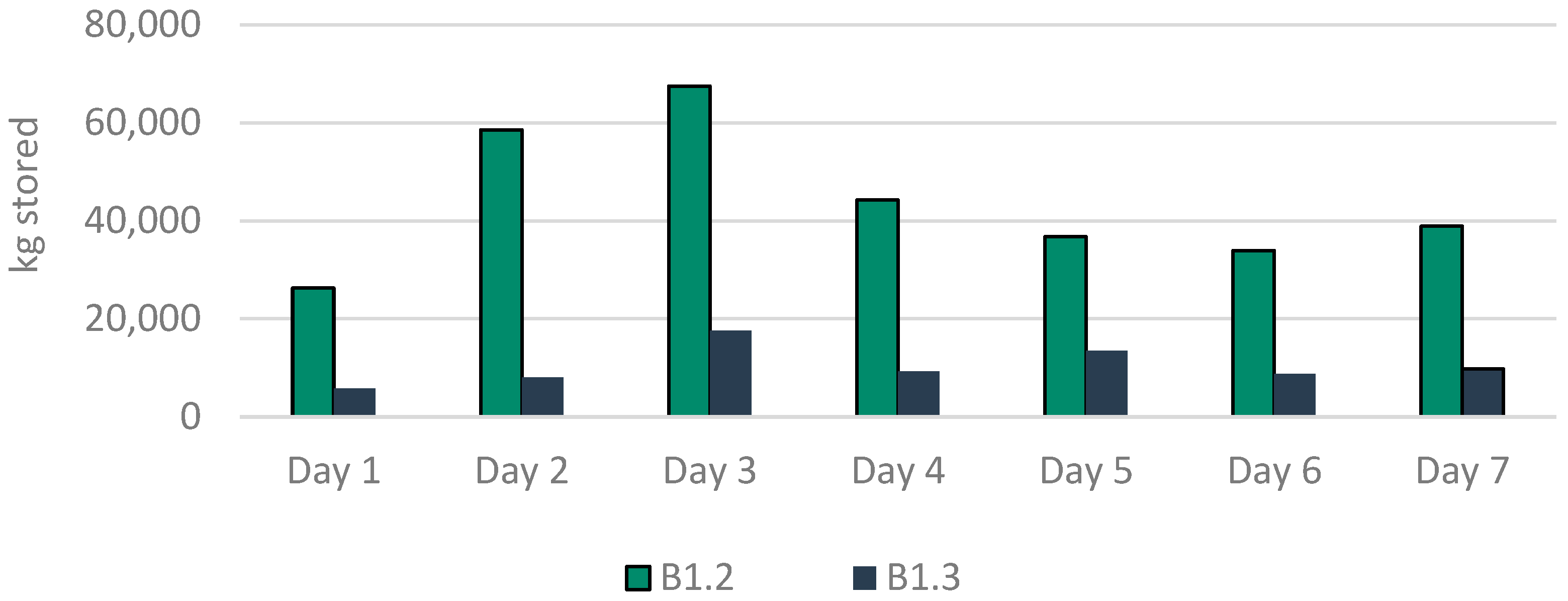
As observed in Figure 8, the operating cost seems to comprise the majority of the total production cost. Line utilization costs are miniscule (1–2 thousand) and therefore they are not visible in the figure. The quality of the scheduling decisions does not affect the operating cost; hence, narrow margins for optimization are left. Once again, inventory and changeover costs, and therefore the schedule quality, vary depending on the user’s knowledge of the production process. Significantly larger volumes of products seem to be stored when the schedule is derived using the rule-based software, as shown in Figure 9. Although this might not lead to remarkable increases in production costs, warehouse capacity issues may emerge in the future, especially due to the large number of products left stored at the end of the scheduling horizon.

As summarized in

Table 12. Production cost reduction due to capacity expansion of the TYRAS facility.

Initial Capacity	Extra Line Identical to Line 2
B1.2	(B2.2)	−0.86%
B1.3	(B2.3)	−0.27%

, capacity expansion decisions result in a minor production cost reduction for both solution approaches. Cost minimization is achieved using the optimization-based approach. In this case, production capacity should be only decided on the basis of achieving increased product demand and not on cost reduction benefits.

It is also worth comparing the computational performance of the two approaches. Both approaches generate feasible schedules; however, SchedulePro^TM can derive a production plan practically instantaneously. On the other hand, the computation time required by the optimization method is quite longer and depends on the problem’s complexity. For the problems examined, the computation time of both approaches is acceptable and perfectly compatible with weekly production scheduling. Nevertheless, this would not necessarily be the case for larger and more complex industrial problems. An important characteristic of the rule-based approach is the solution speed, which is critical for the industrial application of a scheduling solution and remains the same despite the size of the problem. As a result, the CPU time reduction when using SchedulePro^TM, compared to the proposed optimization method, is significant for more complex problems.

Furthermore, the dynamic nature of industrial environments sometimes requires online reactive scheduling due to frequent occurring unexpected changes, e.g., equipment malfunctions, order cancellations, new or updated orders etc., resulting in the need for fast solutions, within seconds, to prevent production stoppages. In this case, immediate decisions have to be made, making the slower MILP framework an unfavorable choice. However, if there is no need for instantaneous decisions, production engineers should consider the fact that optimization methods, while lacking the speed of rule-based approaches, especially when dealing with large industrial problems, generate optimal scheduling plans, which translate to a significant reduction in production costs.

5. Conclusions

The performance of food processing plants depends on operators and managers making correct and timely decisions. Without computer-aided scheduling tools, production staff cannot see the full consequences of their actions. As a result, productivity is reduced, customers are disappointed, and profits suffer. The work discusses two different knowledge-based approaches providing expert information to assist operators and production management, in multi-stage, multi-product food industries, to make decisions in complex production operating environments. More specifically, an optimization and a rule-based approach are used to generate feasible production schedules for two yoghurt production industries, with easy modification of the schedule, constituting an important asset of the latter approach.

It is concluded that the rule-based approach provides feasible solutions in much shorter times compared with the optimization-based approach. Nevertheless, production cost minimization, under existing tight profit margins, can only be achieved by using optimization-based methods. If rule-based approaches are to be used, it is essential to translate engineers’ and operators’ knowledge into heuristic rules in order to improve the solution quality. In dynamic industrial environments, the need for online reactive scheduling may arise due to frequent changes, requiring fast solutions to avoid production disruptions. In such cases, the slower MILP framework might not be suitable compared to the ruled-based approach. However, when dealing with offline scheduling where immediate decisions are not required, production engineers should consider that while optimization methods may be slower than rule-based approaches, they generate optimal scheduling plans that lead to significant cost reductions. Better overall results could be achieved by employing optimization-based methods to derive an initial weekly plan and rule-based approaches to update the plan in real time when dynamic changes occur.

The importance of industries to provide adequate training to their production engineers and scheduling managers has been revealed in the context of this work. Food industries are required to make investments toward the integration of scheduling technologies with plant data and training of their staff on the use of scheduling software and optimization-based approaches. The acceptance of these techniques by the decision makers is due to the lack of understanding of recent developments in the area, thus leading to reluctance to trust the new methods. The benefits of optimization-based scheduling techniques to food producers are easy to appreciate, including a reduction in energy consumption, idle times and changeover times as well as an increase in profits.

Finally, the results of the work illustrate the need to bridge the gap between industrial practice and academic research. In conclusion, both solution methods are deemed as effective for handling complex large-scale industrial scheduling problems, which are typically met in food industries. However, the complexity of the problem and the user experience can significantly impact the quality and computational cost of the solution provided. The comparison between the two methods is solely based on the solution time, production cost and training requirements. A key direction for future extension would be the development of an integrated optimization/rule-based framework to explore their synergistic benefits and derive complex scheduling decisions of high quality in low computation times.