A Novel Model Prediction and Migration Method for Multi-Mode Nonlinear Time-Delay Processes

Abstract

Most industrial processes have nonlinear and time-delay characteristics leading to difficulty in prediction modeling. In addition, the working conditions of most industrial processes are complex, which results in multiple modes. Testing and modeling for each mode is a waste of time and resources. Therefore, it is urgent to complete model migration between different modes. In this work, a new prediction model, a nonlinear autoregressive model with exogenous inputs and back propagation neural network (NARX-BP), is proposed for the nonlinear and time-delay processes, where the input data order of the model is determined by the feedforward neural network (FNN) method, and the nonlinear relation is realized by the BP neural network. For the multi-mode characteristic, a new migration optimization algorithm, input–output slope/bias correction and differential evolution (IOSBC-DE), is provided for using a small amount of data under a new mode to correct the slope and bias of the relationship between the input and output variables through DE. The modeling and migration methods are applied to a wind tunnel system, and the simulation result shows the effectiveness of the proposed method.

1. Introduction

At present, industrial manufacturing is progressing towards high integration, deep automation, digitization, and intelligence. This is achieved through the utilization of various electronic sensing devices with high accuracy and advanced control systems, enabling real-time collection and analysis of production process data in factories. Industrial automation has become increasingly mature and is rapidly advancing toward intellectualization. In order to enhance competitiveness and achieve control objectives within the same industry, strict control over industrial production facilities is necessary to meet customer demands [1]. With the continuous proliferation and upgrading of data acquisition equipment, industrial process datasets have become more complex. These datasets exhibit highly nonlinear and time-delay characteristics, along with a variety of parameters, resulting in the emergence of multiple operational modes. In this context, the application of predictive modeling technology and the exploration of migration models have become inevitable trends.

Predictive modeling offers the ability to predict target variables by utilizing relevant and easily measurable process variables, thereby avoiding the inconvenience of direct measurement. This technology has found applications in certain industrial processes. However, the majority of controlled processes in the process industry exhibit nonlinear and time-delay characteristics. Traditional linear methods typically assume that the industrial process operates near a stable operating point, with variables exhibiting approximately linear correlations within a narrow range. However, nonlinearities are prevalent in industrial systems, and time delay is a common occurrence. Time delay can degrade the performance of closed-loop systems and even lead to their instability. Modeling nonlinear systems with time delay is thus a significant area of research within the field of automatic control.

Model prediction in industrial processes involves predicting target variables based on input variables. The concept of model prediction was initially introduced by Brosilow and Tong [2]. However, this method assumes a linear relationship between output and input variables, which is often not the case in real industrial processes. Nonlinearity and time delay are common occurrences in industrial processes, making a simple linear model inadequate for meeting practical requirements. Consequently, numerous researchers have conducted extensive studies on the prediction of nonlinear and time-delay systems in industrial processes. For example, Xiang proposed a time-delay nonlinear backpropagation (BP) neural network model, which was utilized to predict the import and export trade development trends of an electronic product [3]. Xu, considering the time-delay nonlinear characteristics of rail transit passenger flow, employed support vector regression (SVR), non-autoregressive (NAR), and nonlinear autoregressive network with exogenous inputs (NARX) models to predict passenger flow, with the NARX model demonstrating higher accuracy [4]. Fu and Zhu developed a caving height prediction model for surrounding rock in caving mining at the Xiadian gold mine based on the time-delay nonlinear MGM model theory. However, the prediction accuracy of the model may be affected as disturbances continuously enter the system over time, resulting in an increased signal-to-noise ratio (SNR) [5]. In the study by Luo and Ding, they considered the nonlinear and time-delay characteristics of groundwater resource accumulation and proposed the GM model by combining grey system theory with the time-delay phenomenon [6]. These examples highlight the efforts of researchers to address the challenges posed by nonlinear and time-delay systems in industrial process prediction, utilizing various modeling approaches to improve accuracy and effectiveness.

Although significant progress has been made in the predictive modeling of nonlinear systems with time delays, there are still some shortcomings that need to be addressed. Firstly, the majority of existing prediction models primarily focus on minimizing training sample errors as their main criterion. However, this approach often results in poor generalization ability for the prediction models. Therefore, BP neural network with strong generalization ability rises with it. The BP neural network was proposed by Rumelhart in 1986 [7]. To address the limitations mentioned earlier, researchers have explored alternative approaches. One such approach is transforming the original forward modeling method into a self-supervised learning process that incorporates feedback. This is achieved through the concept of result forward propagation and error back propagation. Despite the emergence of various machine learning methods, the backpropagation (BP) neural network remains an important algorithm for tackling nonlinear problems [8]. Another aspect to consider is the dynamic and time-delay nature of complex industrial processes. In time series modeling, a widely utilized method is the Nonlinear Autoregressive model with eXogenous inputs (NARX) [9]. This method exhibits excellent learning and memory capabilities, as well as delayed feedback functions, enabling it to effectively describe the strong nonlinear dynamics often present in industrial processes. By incorporating nonlinear data-driven learning, NARX makes significant contributions to addressing time-delay problems within systems.

Moreover, due to the complex system setting parameters, the system characteristics change greatly under different working conditions, so the problem of multiple modes arises. With the development of various technologies, enterprises and society have higher and higher requirements for the quality of products, which means that the accuracy of establishing prediction models for industrial process data is higher and higher. For different modes, the process modeling based on data must be repeated, and a large number of experiments must be repeated to develop new models. Obviously, this is inefficient and uneconomical. Therefore, in order to save time and reduce costs, it is necessary to study the migration algorithm.

The model migration method serves to optimize the basic model established using known source domain data and derive a model suitable for the target domain based on data from new working conditions [10]. Researchers such as Luo, Yao, and Gao utilized Bayesian algorithms to extract the most statistically valuable information from data with similar properties. This information was then employed to estimate relevant data for the migration model [11]. In the context of battery operation modes, Tang et al. successfully migrated an accelerated aging model to describe normal speed aging behavior via the Bayesian Monte Carlo algorithm. They parameterized the new model within this framework and used it to predict the aging trajectory of the remaining batteries [12]. To address the issue of multiple working conditions in a wind tunnel control system, Ju, Wang, and Gao developed multiple sub-models. They implemented a scheduling mechanism that selects the closest local model based on the actual situation. However, this modeling method does not ensure the inclusion of all local models [13]. Yu proposed a cross-mode biomedical image multi-label classification algorithm. This method captured pattern characteristics from image content and explanatory text, introduced both homogeneous and heterogeneous data for transfer learning, and alleviated problems arising from small annotation data scales and imbalanced label distributions in the biomedical image field. However, in the case of incomplete data in industrial processes, ensuring accurate feature division becomes challenging [14]. Therefore, there is a need for a model migration method that has lower requirements regarding data characteristics and features a simpler structure. This would allow for effective model migration in situations where data may be incomplete or challenging to work with.

The input–output slope bias correction (IOSBC) method was first proposed by Gao for the injection molding process [15,16]. The mentioned method treats the new process as a shift and scaling of the historical process. With a small amount of data from the new process, the slope and bias parameters of the relationship between the input and output variables can be corrected. This correction process requires finding the optimal slope and bias parameters, which involves iterative operations. However, traditional iterative methods can sometimes get stuck in local minima, leading to a phenomenon known as a “dead cycle” that prevents further progress. To overcome this limitation, global optimization algorithms such as Genetic Algorithm (GA) and Particle Swarm Optimization (PSO) are commonly used [17]. However, compared to GA and PSO, Differential Evolution (DE) stands out as a more user-friendly, faster, and more powerful optimization technique [18]. DE can effectively search for the global optimum by maintaining a population of candidate solutions and iteratively improving them. Its simplicity and efficiency make it a preferred choice for optimizing the parameters in the context of model migration and adjustment.

In order to establish a prediction model for nonlinear and time-delayed industrial data and achieve model migration under different operating conditions to obtain accurate prediction models in all conditions, this article first employs the NARX model as the predictive model structure and the False Nearest Neighbor (FNN) algorithm to determine the order of input variables. The BP neural network is then used as the nonlinear fitting function of the NARX model to establish the predictive model under historical operating conditions. Based on the historical operating model and a small amount of new operating condition data, this article proposes a new model migration method, IOSBC-DE. This method uses the IOSBC structure as the mapping relationship between the historical model and the new model, combines a small amount of data from new operating conditions, and utilizes the DE algorithm with global optimization characteristics to optimize the bias slope in the new model and establish a prediction model for the new operating condition. Finally, the method is applied to real wind tunnel tests to verify the effectiveness of the strategy. The method proposed in this paper is easy to implement and provides a feasible technical approach for precise control of industrial systems in various modes.

2. Methodology

In order to achieve prediction of complex industrial data under harsh operating conditions, it is necessary to first establish a prediction model suitable for nonlinear and time-delayed industrial process scenarios. Furthermore, to accurately predict data under multiple operating conditions in industrial processes, transfer learning for the prediction model is required. In this section, the establishment of NARX-BP model and the implementation of IOSBC-DE migration algorithm are introduced.

2.1. Establishment of NARX-BP Model

The NARX model can provide accurate predictions for short time series, which has important applications in solving the modeling of systems with nonlinear and time-delay characteristics. The basic equation of NARX network for time series prediction can be expressed as follows:

$$\widehat{\mathbf{y}}\left(t\right)=\Psi \left(y\right(t-1),\dots ,y(t-n_y),u(t-1),\dots ,u(t-n_u\left)\right)$$

(1)

where $y(t-1),\dots ,y(t-n_y)$ and $u(t-1),\dots ,u(t-n_u)$, respectively, represent the measurement output and input sequence of the system; $n_u,n_y$ represent the order of input and output variables at the past time, respectively; $\widehat{y}(t)$ represents the prediction output; $\psi$ represents the nonlinear function.

The structure of NARX model is shown in Figure 1.

In the NARX model, the selection of variable order and nonlinear function significantly impacts the model’s accuracy. In theory, a higher order can capture more information and better describe system characteristics. However, an excessively large order can lead to exponential data growth and increased noise. Hence, it is crucial to carefully select the appropriate order for modeling. Several commonly used methods for order determination include the correlation integral (CI) method [19], singular value decomposition (SVD) method [20], and the FNN method.

The CI method requires a substantial sample size and is susceptible to noise. The SVD method, being inherently linear, is not suitable for nonlinear systems. In this paper, the FNN method is employed to determine the variable order. The FNN method calculates the distance correlation before and after feature selection for each variable, evaluating the original feature’s explanatory ability for the target variable. Hence, the FNN method is chosen as the order determination technique.

When selecting the nonlinear function, it is crucial to avoid overfitting and ensure the model possesses fault tolerance. The BP neural network exhibits a reasonable fault tolerance and is well-suited for capturing nonlinear mapping relationships.

Therefore, this paper employs NARX-BP neural network as the prediction model of nonlinear and time-delayed industrial conditions. The input data of the NARX model structure is determined by the FNN method, and the BP neural network is used as nonlinear function.

The design process of the NARX-BP model under a single mode is shown in Figure 2.

Given the time series $X={[x_{(1)},\dots ,x_{(k)}]}^{\mathrm{T}}$, suppose that one point $x_{(j)}$ in n dimensional space is the nearest point of another point $x_{(i)}$. The distance between them is $d_n=\left|\right|x_{(j)}-x_{(i)}|{|}^{(n)}$. When the dimension increases to n + 1, the distance between them becomes $d_{n+1}=\left|\right|x_{(j)}-x_{(i)}|{|}^{(n+1)}$. If $d_{n+1}$ is much larger than $d_n$, it can be considered that this is caused by the fact that the two non-adjacent points in the high-dimensional attractor become adjacent points after being projected onto the low-dimensional line. Such points are false. Therefore, if Equation (2) holds, $x_{(j)}$ is the false nearest neighbor of $x_{(i)}$, where R is the threshold, usually between 10 and 50 [21].

$$\sqrt{\frac{d_{n+1}^2-d_n^2}{d_{n+1}^2}}\ge R$$

(2)

Starting from n = 1, the ratio of false nearest neighbor points is calculated until the ratio of false nearest neighbor points is less than 5% or the false nearest neighbor points do not decrease with the increase of dimension. Then, the geometric structure of the attractor can be considered to be completely open, and n at this time is selected as variable order.

If there are n process variables $x_1,\dots ,x_n$, q output variables $y_1,\dots ,y_q$, the orders of variables determined by the FNN method $n_1,\dots ,n_n$ and $n_{o1},\dots ,n_{oq}$, the input of the model $\mathbf{r}(k)$ can be expressed as:

$$\begin{array}{ll}\mathbf{r}(k)=& (x_1(k-1),\dots ,x_1(k-n_1),\dots ,x_n(k-1),\dots ,x_n(k-n_n),\\ & y_1(k-1),\dots ,y_1(k-n_{o1}),\dots ,y_q(k-1),\dots ,y_q(k-n_{oq}))\end{array}$$

(3)

According to the input of the model, the number of input layers can be determined as $r$, $r=n_1+\dots +n_n+n_{o1}+\dots +n_{oq}$; the number of output layers can be determined as $q$, which is the number of output variables; the number of middle layers can be determined as $h$. Generally, the selection of the number of middle layers is calculated according to the following equation:

$$h=\sqrt{r+q}+a$$

(4)

where a is constant between 1 and 10, usually set around 5 [22].

Through the nonlinear mapping of the model, the output vector of the output layers at time k, $\mathbf{y}\left(k\right)=\left(y_1\right(k),\dots ,y_q(k\left)\right)$ is calculated:

$$\mathbf{y}\left(k\right)=f_o\left({\mathbf{W}}_{mo}^k\right(f_m\left({\mathbf{W}}_{im}^k\mathbf{r}\right(k)-{\mathbf{b}}_m^k(k\left)\right)-{\mathbf{b}}_o^k)$$

(5)

$$W_{mo}^k(q\times h)=\left(\begin{array}{ccc}{w}_{11}^{\prime k}& \cdots & w_{1h}^{\prime k}\\ ⋮& \ddots & ⋮\\ w_{q1}^{\prime k}& \cdots & w_{qh}^{\prime k}\end{array}\right)$$

(6)

$$W_{im}^k(h\times c)=\left(\begin{array}{ccc}{w}_{11}^k& \cdots & w_{1r}^k\\ ⋮& \ddots & ⋮\\ w_{h1}^k& \cdots & w_{hr}^k\end{array}\right)$$

(7)

$$b_m^k(h\times 1)=\left(\begin{array}{c}{b}_1^k\\ ⋮\\ b_h^k\end{array}\right)$$

(8)

$$b_o^k(q\times 1)=\left(\begin{array}{c}{b}_1^{\prime k}\\ ⋮\\ b_q^{\prime k}\end{array}\right)$$

(9)

where $f_o$ is the mapping function selected from the middle layers to the output layers; ${\mathbf{W}}_{mo}^k$ is the link weight matrix between the middle layers and the output layers; $f_m$ is the mapping function selected from the input layers to the middle layers; ${\mathbf{W}}_{im}^k$ is the link weight matrix between the input layers and the middle layers; ${\mathbf{b}}_m^k$ is the threshold matrix of each neuron in the middle layers; ${\mathbf{b}}_o^k$ is the threshold matrix of each neuron in the output layers.

Then, the gradient descent method is used to update the link weight matrix ${\mathbf{W}}_{mo}^k$, ${\mathbf{W}}_{im}^k$ and the threshold matrix ${\mathbf{b}}_m^k$,${\mathbf{b}}_o^k$.

$$e(k)=\frac{1}{2q}{\displaystyle \sum _{c=1}^q{(y_c(k)-\overline{y_c}(k))}^2}$$

(10)

$${\mathbf{W}}_{mo}^{k+1}={\mathbf{W}}_{mo}^k+\Delta {\mathbf{W}}_{mo}^k={\mathbf{W}}_{mo}^k-\mu \frac{\partial e(k)}{\partial {\mathbf{W}}_{mo}^k}$$

(11)

$${\mathbf{W}}_{im}^{k+1}={\mathbf{W}}_{im}^k+\Delta {\mathbf{W}}_{im}^k={\mathbf{W}}_{im}^k-\mu \frac{\partial e(k)}{\partial {\mathbf{W}}_{im}^k}$$

(12)

$${\mathbf{b}}_m^{k+1}={\mathbf{b}}_m^k+\Delta {\mathbf{b}}_m^k={\mathbf{b}}_m^k-\mu \frac{\partial e(k)}{\partial {\mathbf{b}}_m^k}$$

(13)

$${\mathbf{b}}_o^{k+1}={\mathbf{b}}_o^k+\Delta {\mathbf{b}}_o^k={\mathbf{b}}_o^k-\mu \frac{\partial e(k)}{\partial {\mathbf{b}}_o^k}$$

(14)

where $e(k)$ is the prediction error obtained from the k-th training. $y_c(k)$ is the actual output; $\overline{y_c}(k)$ is the model output; $\mu$ is the learning rate, usually between 0.01 and 0.8 [23].

Suppose the number of data samples is K. The first iteration is completed to obtain the weight matrix ${\mathbf{W}}_{mo}^K$, ${\mathbf{W}}_{im}^K$ and the threshold matrix ${\mathbf{b}}_m^K$, ${\mathbf{b}}_o^K$ of the model. Then, the global output $\overline{y_c}(k)$ of the model is calculated as follows:

$$\overline{y_c}(k)=f_o(W_{mo}^K(f_m(W_{im}^{K}r(k)-b_m^K))-b_o^K)$$

(15)

where $k=1,\dots ,K$. The global error E is calculated as follows:

$$E=\frac{1}{2K}{\displaystyle \sum _{k=1}^K{\displaystyle \sum _{c=1}^q{(y_c(k)-\overline{y_c}(k))}^2}}$$

(16)

If the global error E is greater than the set minimum error E_min, and the set number of iterations N has not been reached, the next iteration begins. Until the global error E is less than the set minimum error E_min or the number of iterations N has been reached, the calculation stops. The optimal weight matrix and threshold matrix are obtained.

$$W_{mo}^{}=\left(\begin{array}{ccc}{w}_{11}^{\prime }& \cdots & w_{1h}^{\prime }\\ ⋮& \ddots & ⋮\\ w_{q1}^{\prime }& \cdots & w_{qh}^{\prime }\end{array}\right), W_{im}^{}=\left(\begin{array}{ccc}{w}_{11}^{}& \cdots & w_{1r}^{}\\ ⋮& \ddots & ⋮\\ w_{h1}^{}& \cdots & w_{hr}^{}\end{array}\right), b_m=\left(\begin{array}{l}{b}_1\\ ⋮\\ b_h\end{array}\right), b_o=\left(\begin{array}{l}{b}_1^{\prime }\\ ⋮\\ b_q^{\prime }\end{array}\right)$$

(17)

The output of the final model is expressed as follows:

$$\overline{y}\left(k\right)=f_o(W_{mo}^{}(f_m(W_{im}^{}r(k)-b_m^{}))-b_o^{})$$

(18)

To sum up, the model parameters and structure are determined as shown in Figure 3.

2.2. Implementation of Model Migration

Based on the NARX-BP model discussed earlier, an accurate basic model for a single mode is established. However, when a new mode arises and limited operating data becomes available, the Input–Output Structure-Based Cooperation (IOSBC) method is employed to establish the parameter relationship between the basic model and the new model. Similar to Genetic Algorithm (GA), Differential Evolution (DE) exhibits the capability to be easily combined with other algorithms, making it suitable for optimizing parameters within the IOSBC method.

Therefore, this paper proposes a novel migration optimization algorithm called IOSBC-DE. This algorithm effectively migrates the model based on limited data, meeting the required level of accuracy. The model migration design process is illustrated in Figure 4.

The IOSBC method obtains the model under the new mode according to the basic model. The basic NARX-BP model established under a single mode is (13). The optimal weights and thresholds of the basic model are ${\mathbf{W}}_{mo}$, ${\mathbf{W}}_{im}$, ${\mathbf{b}}_m$, and ${\mathbf{b}}_o$.

The weight of the input layers to the middle layers under the new mode model is defined as ${\mathbf{V}}_{im}$ and the threshold is ${\mathbf{c}}_m$. The weight of the middle layers to the output layers is ${\mathbf{V}}_{mo}$ and the threshold is ${\mathbf{c}}_o$.

$$V_{im}=\left(\begin{array}{ccc}{s}_{11}^{}\times w_{11}^{}+b_{11}^{}& \cdots & s_{1r}^{}\times w_{1r}^{}+b_{1r}^{}\\ ⋮& \ddots & ⋮\\ s_{h1}^{}\times w_{h1}^{}+b_{h1}^{}& \cdots & s_{hr}^{}\times w_{hr}^{}+b_{hr}^{}\end{array}\right)$$

(19)

$$c_m=\left(\begin{array}{c}{s}_{m1}\times b_1+b_{m1}\\ ⋮\\ s_{mh}\times b_h^{}+b_{mh}\end{array}\right)$$

(20)

$$V_{mo}=\left(\begin{array}{ccc}{s}_{11}^{\prime }\times w_{11}^{\prime }+b_{11}^{\prime }& \cdots & s_{1h}^{\prime }\times w_{1h}^{\prime }+b_{1h}^{\prime }\\ ⋮& \ddots & ⋮\\ s_{q1}^{\prime }\times w_{q1}^{\prime }+b_{q1}^{\prime }& \cdots & s_{qh}^{\prime }\times w_{qh}^{\prime }+b_{qh}^{\prime }\end{array}\right)$$

(21)

$$c_o=\left(\begin{array}{c}{s}_{o1}\times b_1^{\prime }+b_{o1}\\ ⋮\\ s_{oq}\times b_q^{\prime }+b_{oq}\end{array}\right)$$

(22)

where $s_{ij}^{}$, $b_{ij}^{}$, $s_{mi}^{}$, and $b_{mi}^{}$ (I = 1…h; j = 1…r) are the migration coefficients of the weights and thresholds of the input layers to the middle layers, and $s_{pi}^{\prime }$, $b_{pi}^{\prime }$, $s_{op}^{}$, and $b_{op}^{}$(i = 1…h; p = 1…q) are the migration coefficients of the middle layers to the output layers.

For the calculation of the migration coefficients, DE is used to find the optimal solution via a small amount of data on the new mode.

First, the initial population is randomly generated, and the population size is denoted as P. The general value range is 20 to 100. Then, the most common binary encoding method is used to complete the encoding and decoding design. Then, the fitness error corresponding to the pop-th individual is calculated, pop = 1, …, P. The fitness error function usually selects the average value of the square of the prediction error.

$$Fitnes{s}^{pop}=\frac{1}{K}{\displaystyle \sum _k^K{\left[y_{new}\left(k\right)-{\overline{y}}_{new}\left(k\right)\right]}^2}$$

(23)

$${\overline{y}}_{new}^{pop}\left(k\right)=f_o(V_{mo}^{pop}(f_h(W_{im}^{pop}{r}_{new}(k)-c_m^{pop}))-c_o^{pop})$$

(24)

where $y_{new}\left(k\right)$ is the actual measured value under the new mode at time k; ${\overline{y}}_{new}^{pop}\left(k\right)$ is the output of the new mode calculated under the pop-th individual at time k; $r_{new}\left(k\right)$ is the input under the new mode. $V_{im}^{pop}$, $c_m^{pop}$, $V_{mo}^{pop}$, and $c_o^{pop}$ are the weights and thresholds defined by the pop-th individual in the population.

During the model migration process, the initial population size Np of the differential evolution algorithm is set to 80, the initial relative scale factor F is set to 0.3, and the initial crossover factor Cr is set to 0.5. The number of iterations Gm is set to 80. In order to ensure a higher optimization success rate and faster convergence speed, an adaptive factor that varies with the number of iterations is selected to be used. The expressions are listed as follows:

$$F=F_0·2^{exp(1-\frac{Gm}{1+Gm-G})}$$

(25)

$$Cr={\left(\frac{G-1}{Gm}\right)}^2$$

(26)

where $F_0$ is initial relative scale factor and G is current number of iterations.

In a wind tunnel system, the most important thing is the stability of the Mach number. Therefore, it is required to minimize the error between the output value and the predicted value and select the average of the error squares as the fitness function. In order to quickly find the migration model with the best fitness, select DE/test/2 as the mutation strategy, which is defined as follows:

$$v_i^{\left(G\right)}={x_{best}}^{\left(G\right)}+F({x_{{R_1}^i}}^{\left(G\right)}-{x_{{R_2}^i}}^{\left(G\right)})+F({x_{{R_3}^i}}^{\left(G\right)}-{x_{{R_4}^i}}^{\left(G\right)})$$

(27)

After initialization, DE creates a donor/mutant vector $v_i^{\left(G\right)}$ corresponding to each population member or target vector ${x_i}^{\left(G\right)}$ in the G-th iteration through mutation.

The indices ${R_1}^i$, ${R_2}^i$, ${R_3}^i$, and ${R_4}^i$ are mutually exclusive integers randomly chosen from the range [1, Np], and all are different from the base index i. These indices are randomly generated anew for each donor vector. ${x_{best}}^{\left(G\right)}$ is the best individual vector with the best fitness in the population at G-th iteration [24].

Then, the fitness function and the number of iterations are judged until a certain set value is reached to complete the cycle. At this time, the optimal migration correction parameters of the weights and thresholds of the basic model are obtained, and then the optimal weights and thresholds of the new model are obtained, marked as $V_{im}^{best}$, $c_m^{best}$, $V_{mo}^{best}$, and $c_o^{best}$ At this time, the model of the new mode is expressed as follows:

$${\overline{y}}_{new}^{best}\left(k\right)=f_o(V_{mo}^{best}(f_h(W_{im}^{best}{r}_{new}(k)-c_m^{best}))-c_o^{best})$$

(28)

In conclusion, according to the determined NARX-BP model and the advantages of IOSBC-DE method, the migration optimization algorithm under multiple modes is designed. Utilizing a small amount of operating data obtained under the new mode, the optimal weights and thresholds of the new model are determined.

2.3. Model Evaluation Index

For a complex system, in order to judge whether it reaches the best level, the model evaluation index is needed. Generally, the root mean square error (RMSE) is selected as the evaluation index. The smaller the RMSE is, the more accurate the model is:

$$RMSE=\sqrt{\frac{1}{K}{\displaystyle \sum _{k=1}^K{(y(k)-\overline{y}(k))}^2}}$$

(29)

where $y(k)$ indicates the actual value, $\overline{y}(k)$ represents the predicted value, and K represents the number of samples.

On the other hand, the purpose of model prediction is to control. Usually, there is a set value for the output variable, which is recorded as $y_{set}$. When putting the model into the controller, the control effect should be evaluated through the accuracy of the model via the indexes accuracy (A) and maximum deviation (MD). A is the deviation between the average predicted value and the set value over time. MD is the maximum predicted deviation between the actual value and the predicted value during the whole prediction process.

$$A=\left|y_{set}-\frac{1}{K}{\displaystyle \sum _{k=1}^K\overline{y}(k)}\right|$$

(30)

$$MD=\max \left|y(k)-\overline{y}(k)\right|$$

(31)

3. Process Description of Wind Tunnel System

The wind tunnel is an annular tubular experimental device used to artificially generate and control airflow, simulating the airflow around aircraft or objects. It allows for the measurement of the airflow’s impact on the object and the observation of physical phenomena. The wind tunnel is a typical nonlinear time-delay system with multiple working modes due to various set parameters. Its importance lies in the study of aerodynamics, the analysis and design of aircraft structures, appearance, and material usage. The continuous wind tunnel is powered by compressors, and the airflow within is controlled by the compressor speed. Key process parameters include total pressure, Mach number, and attack angle.

To meet the desired conditions, the wind tunnel is first operated to achieve a stable Mach number, after which the desired change in attack angle is set, and data is collected during this change.

The continuous wind tunnel represents a complex system with multiple variables. The Mach number serves as an important parameter for analyzing the wind tunnel’s flow field performance and acts as a primary control index. During the blowing process in the wind tunnel, the total pressure in the stable section of the flow field is influenced by factors such as gas temperature, gas constant, and gas density. While the gas temperature remains uncontrolled during experiments, the total pressure is primarily adjusted by modifying the gas density. Directly obtaining the Mach number using a mechanistic model in the complex wind tunnel system proves challenging. However, leveraging the knowledge of aerodynamic theory allows for calculating a more accurate Mach number by considering the total pressure and static pressure.

Currently, the total pressure in the continuous wind tunnel is controlled independently, and changes in total pressure significantly impact the Mach number. The compressor speed, in turn, affects the static pressure. Additionally, the attack angle refers to the angle between the wing and the direction of airflow when an aircraft model is positioned within the test section. Precise control of the attack angle is crucial for aircraft model startup testing. The main influential variables are summarized in

Table 1. Key variables of wind tunnel process.

No.	Variable Description	Unit
1	Mach number (Ma)	/
2	Total pressure (P0)	kPa
3	Speed (Sp)	r/s
4	Attack angle (Att)	°

.

4. Results and Discussion

In the wind tunnel flow field, the flow field characteristics change greatly under different working modes. Due to the special needs of the experimental model, the set value of the Mach number is different, which has caused great difficulties in the establishment of the model.

In this paper, the experimental transonic data with Mach number operating parameters ranging from 0.6 to 1.0 are studied, with the injection gap set at 24 mm. The opening to closing ratio is set to 1.5%. The attack angle ranges from −4° to 10°. According to different Mach number set values, the selection of test conditions and the number of samples are shown in

Table 2. Different modes.

Mode Number	Ma Set Value	Number of Samples
1	0.6	1261
2	0.7	2717
3	0.75	1989
4	0.8	985
5	0.85	2113
6	0.9	1451
7	0.95	1455
8	1.0	965

.

4.1. Ma Prediction Results Based on NARX-BP Model

According to the actual operation process of the wind tunnel and expert experience, the total pressure, speed, and attack angle are the input variables, and the Mach number is the output variable of the model. According to the structure of the NARX-BP model, the selection of the order of model variables directly affects the accuracy of the model prediction. The order of model variables is determined via FNN. Taking the Mach number and attack angle order analysis under Mode 1 as an example, the order of the variables is from 1 to 15, and the analysis results are shown in Figure 5. As seen from Figure 5, for Mode 1, the optimal order of the Mach number is 6, and the optimal order of the attack angle is 6.

Similarly, the FNN method is used to analyze all variables under all modes. The results are shown in

Table 3. Order analysis of model variables.

Test Number	Ma (nma)	P0 (no)	Sp (nsp)	Att (na)
1	6	3	6	6
2	5	4	8	4
3	5	5	6	5
4	4	5	6	4
5	4	4	5	5
6	3	3	6	4
7	5	4	7	5
8	3	4	7	5

.

As seen from the above table, the order of each variable is slightly different under different modes, but the order of the same variable can change by up to three orders under different modes. In order to better reflect the applicability of the selected order, the mode of the orders of each variable under different modes is selected as the final order of the model, and the optimal order of the variables is shown in

Table 4. Optimal orders of variables.

Variable	Ma (nma)	P0 (no)	Sp (nsp)	Att (na)
Optimal order	5	4	6	5

.

According to the optimal order of the variables, the number of input layers of the NARX-BP neural network is determined to be 20, the number of output layers is 1, and the number of middle layers is 10 calculated via Equation (4).

Taking Mode 5 as an example, 70% of the data is selected for training, and 30% of the data is tested. The prediction results of the proposed model are compared with the prediction results of the BP neural network and PLS regression prediction adopted in previous related work [25], as shown in Figure 6. As seen from Figure 6a, the changing trend of the predicted Mach number is closer to the actual Mach number via the proposed method. In contrast, the changing trend of the predicted Mach number via the BP network method and the PLS method is quite different from the actual Mach number. It can be seen from Figure 6b that the error between the predicted Mach number and the actual Mach number calculated via the proposed method is less than that predicted via the BP network method and the PLS method.

Similarly, the Mach number prediction of each mode is carried out, respectively, and the prediction model evaluation indexes of each mode are shown in

Table 5. Evaluation indexes of prediction models.

Test Number	BP			PLS			NARX-BP
	RMSE	A	MD	RMSE	A	MD	RMSE	A	MD
1	0.00030	0.00015	0.00081	0.00052	0.00018	0.00139	0.00015	0.00007	0.00063
2	0.00069	0.00044	0.00190	0.00097	0.00071	0.00220	0.00015	0.00008	0.00088
3	0.00019	0.00062	0.00051	0.00036	0.00048	0.00102	0.00011	0.00058	0.00050
4	0.00044	0.00014	0.00132	0.00061	0.00014	0.00156	0.00019	0.00005	0.00064
5	0.00115	0.00067	0.00408	0.00125	0.00107	0.00261	0.00018	0.00004	0.00072
6	0.00068	0.00034	0.00234	0.00150	0.00087	0.00354	0.00018	0.00009	0.00103
7	0.00073	0.00005	0.00309	0.00166	0.00066	0.00431	0.00019	0.00023	0.00182
8	0.00045	0.00031	0.00177	0.00105	0.00047	0.00382	0.00013	0.00017	0.00036

.

According to the above table, the RMSE values of the proposed NARX-BP model are less than 0.001 under all modes. Under each mode, the RMSE value predicted via the NARX-BP model is less than that predicted via the BP network model and the PLS model, which shows that the predicted Mach number of the NARX-BP model is closer to the actual Mach number and the prediction is more accurate. Under a single mode, the A value of the Mach number is analyzed. Except for Mode 3 and Mode 7, the A values of the NARX-BP model are lower than that of the BP network model and the PLS model. In addition, under each mode, the MD between the predicted Mach number and the actual Mach number obtained via the NARX-BP model is less than that predicted via the BP model and the PLS model. In conclusion, the proposed NARX-BP model has more advantages than the BP network model and the PLS model. The NARX-BP model can further improve the ability of Mach number tracking and prediction.

4.2. Model Migration Results of Mach Number Prediction Model

In the wind tunnel, the core equipment is expensive and consumes a significant amount of energy. Conducting a complete test for each working mode and establishing corresponding models would require substantial manpower and material resources. Therefore, it is crucial for researchers to obtain accurate models while minimizing the number of tests. To achieve this goal and reduce costs and energy consumption, the migration algorithm is applied to the Mach number prediction model of the wind tunnel flow field in this study.

Based on the selected modes, Mode 5 is chosen as the historical mode to establish the NARX-BP basic model, while Mode 4 and Mode 6 are selected as the new modes. Only the first 3% of data from each new mode is used for migrating and modifying the basic model to obtain the new prediction model. The remaining data under the new mode is then predicted using the newly obtained model.

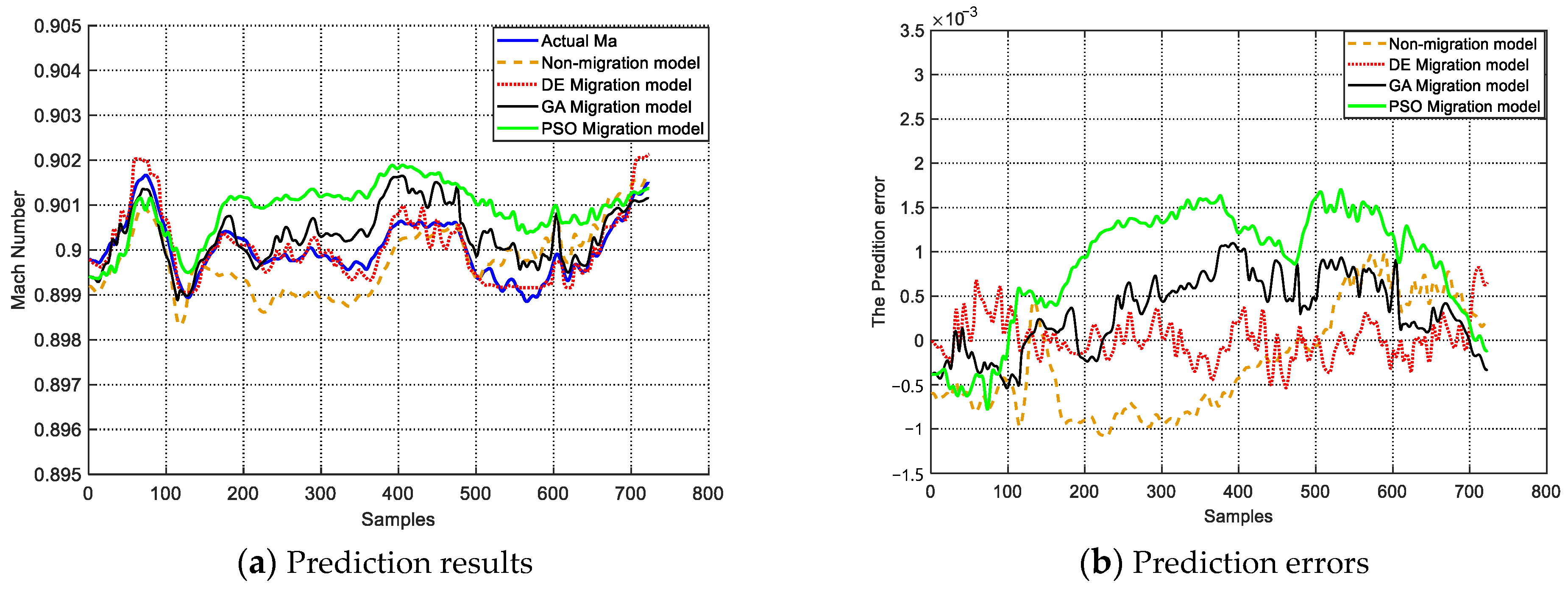
To demonstrate the superiority of the DE model migration, separate NARX-BP models are established for Mode 4 and Mode 6 as new modes, using only 3% of the available data. The prediction results of the DE migration model are compared with the non-migration model established for each mode separately. Additionally, to provide an objective evaluation of the DE algorithm’s performance, the prediction model optimized via DE is compared with prediction models obtained through optimization and screening via GA and PSO algorithms. The prediction results for Mode 4 are presented in Figure 7a, and the corresponding prediction errors are shown in Figure 7b. The prediction results for Mode 6 are depicted in Figure 8a, while the prediction errors are displayed in Figure 8b.

From Figure 7a and Figure 8a, it is evident that when using only a small amount of data from the new modes, both the migration models and non-migration models struggle to accurately reflect the changing trend of the Mach number. However, the predicted Mach number of the migration model is closer to the actual Mach number. Figure 7b and Figure 8b further illustrate that the error in the predicted Mach number via the DE migration model is lower compared to the non-migration model.

The prediction results and evaluation indexes of the above migration model and non-migration model are shown in

Table 6. Evaluation indexes of prediction models.

Test Number	Non-Migration Model			DE Migration Model
	RMSE	A	MD	RMSE	A	MD
4	0.00141	0.00020	0.00358	0.00025	0.00010	0.00074
6	0.00065	0.00263	0.00114	0.00024	0.00005	0.00082

. The prediction results and evaluation indexes of migration models with different optimization algorithms are shown in

Table 7. Evaluation indexes of prediction models optimized via different algorithms.

Test Number	DE Migration Model			GA Migration Model			PSO Migration Model
	RMSE	A	MD	RMSE	A	MD	RMSE	A	MD
4	0.00025	0.00010	0.00074	0.00076	0.00057	0.00194	0.00075	0.00034	0.00130
6	0.00024	0.00005	0.00082	0.00053	0.00035	0.00110	0.00110	0.00090	0.00170

.

When only the first 3% of data are used for the non-migration model, the RMSE values exceed 0.001 under Mode 4 and Mode 6. For the DE migration model, the RMSE can ensure that the prediction result is within 0.001 under Mode 4. Although the RMSE under Mode 6 using the migration model exceeds 0.001, this value is also less than the RMSE of the non-migration model. At the same time, under these two modes, the MD values of the Mach number after model migration are less than the non-migration model. Therefore, the results show that when there is only a small amount of data on the new mode, the migration model method has a better prediction effect.

When comparing DE with GA and PSO optimization methods, it was found that under Mode 4, DE outperformed GA and PSO in three types of evaluation indicators, indicating that the performance of DE in finding globally optimal solutions in the wind tunnel migration model is higher than GA and PSO’s. Through this method, the running time of the test can be greatly reduced, and the blowing cost of the wind tunnel can be saved, which is of great significance to the study of wind tunnel tests.

5. Conclusions

This article presents a novel prediction modeling and migrating method designed to address the nonlinear and time-delay characteristics commonly observed in industrial processes. To tackle multimodal problems, an effective model transfer strategy called IOSBC-DE is proposed. The strategy involves determining the input data order of the NARX model using the FNN method and utilizing a BP neural network as the mapping function. Moreover, the IOSBC method establishes the relationship between historical patterns and new patterns, employing DE optimization to fine-tune slope and bias parameters during the model migration process. Experimental data from wind tunnel processes demonstrate that NARX-BP achieves more accurate predictions for nonlinear and time-delay industrial processes, improving accuracy by 50% (RMSE from 0.00030 to 0.00015) compared to traditional BP neural networks. The migrated model through IOSBC-DE exhibits an 82.3% (RMSE from 0.00141 to 0.00025) increase in prediction accuracy compared to the non-migrated model, with DE outperforming other optimization algorithms in terms of prediction performance. The feasibility of the proposed method is effectively validated.