Article

Effect of Flexible Operation on Residual Life of High-Temperature Components of Power Plants

1
Department of Mechanical Engineering, Jeonbuk National University, 567 Baekje-daero, Deokjin-gu, Jeonju-si 54896, Republic of Korea
2
Carbon Neutral Strategy Department, KEPCO Headquarter, 55 Jeollyeok-ro, Naju-si 58322, Republic of Korea
3
Convergence Technology Laboratory, KEPCO Research Institute, 105 Munji-ro, Yuseong-gu, Daejeon 34056, Republic of Korea
4
Department of Mechanical Engineering, Myongji University, 116 Myongji-ro, Cheoin-gu, Yongin 17058, Republic of Korea
*
Authors to whom correspondence should be addressed.
Processes 2023, 11(6), 1679; https://doi.org/10.3390/pr11061679
Submission received: 21 April 2023 / Revised: 10 May 2023 / Accepted: 24 May 2023 / Published: 31 May 2023
(This article belongs to the Special Issue Reliability and Engineering Applications (Volume II))

Abstract

:
Electricity generation from renewable energy sources is emerging as a result of global carbon emission reduction policies. However, most renewable energy sources are non-dispatchable and cannot be adjusted to meet the fluctuating electricity demands of society. A flexible operation process has been proposed as an effective solution to compensate for the unstable nature of renewable energy sources. Thermal load fluctuations during flexible operation may cause creep–fatigue damage to the high-temperature components of thermal power plants, as they are designed with a focus on creep damage under a constant power level. This study investigated the residual life of high-temperature components, such as a superheater tube and a reheater header, to failure under flexible operation conditions using finite element analysis and empirical models. First, we determined an analytical solution for the straightened superheater tube under thermal conditions and compared it with the numerical solution to verify the numerical models. Through the verified finite element model, the creep–fatigue life of the reheater header was estimated by considering flexible operation factors and employing the Coffin–Manson and Larson–Miller models. Although fatigue damage increases with decreasing minimum load and ramp rate, we confirmed that creep damage significantly affects the residual life during flexible operation. In addition, a surrogate model was proposed to evaluate the residual life of the reheater as a function of the flexible operation factors using the machine learning methodology, based on the results of finite element methods. It can be used to predict its residual life without performing complex thermo-structural analysis and relying on empirical models for fatigue and creep life. We expect our findings to contribute to the efficient operation of thermal power plants by optimizing the flexible operation factors.

1. Introduction

Global CO2 emissions have steadily increased over time, and Belbute [1] has suggested that the emissions will increase by 27.4% by 2030. Prior studies have addressed the adverse effects of fossil fuels on CO2 emissions and the need to generate electricity using renewable energy sources (RES) for low-carbon growth [2,3]. Most RES have non-dispatchable characteristics that prevent them from adjusting the energy supply to meet the demand. Climatic or geographic conditions cause variability in electricity production and can render power plant systems more unstable. According to the average net electricity production per week in Germany in 2021, there was a power fluctuation at approximately 12:00 p.m. owing to the influence of solar power [4]. Τhe concern about power outages caused by over- and under-generation increases with the proportion of RES in the power generation system. As a result, it is critical to address the power uncertainty caused by the increased demand for RES [5]. Flexible operation is a method of changing the output level of a thermal power plant to maintain constant output power according to the change in the output power of the RES. This is the most economical way to handle the instability of RES energy generation [6].
Flexibility indicates the efficiency of a concept. Although higher flexibility addresses the system stability problem, it can be accompanied by thermal load fluctuations that place conventional power plants in harsh conditions. The thermo-structural behavior of these facilities under thermal load variation must be considered as conventional power plants were designed by considering the fatigue and creep of the thermal parts under constant power levels. This study entails an investigation of the thermo-structural behavior of high-temperature components in conventional power plants by using computational analysis, bypassing the time efficiency weakness of practical experiments.
Previous studies primarily focused on assessing the life of power plants. In particular, researchers investigated the unsteady temperature and pressure changes in the superheater header during operation. They concluded that shutdown would cause significant damage to the plant components [7,8]. These studies have helped resolve the structural stability problems caused by creep–fatigue damage during power plant operation. However, these analyses were performed at a general load, and it was impossible to predict the change in the residual life of the plant component under flexible operating conditions. Several researchers [9,10,11,12,13] have studied the cumulative damage of each boiler component through a numerical approach. In addition, prior research focused on the thermo-structural fatigue life under specific loading conditions. Still, it did not evaluate the fatigue and creep life of high-temperature components under fluctuating thermal loading conditions. They described the risk of failure by focusing on creep–fatigue damage accumulation in the boiler header part and performed a quantitative evaluation of the residual life under specific boundary conditions. Although they performed a quantitative assessment of the residual life for different boundary conditions, previous works disregarded the variation in critical life to failure due to changes in thermo-structural conditions.
Recently, studies on flexible operations have progressed. Avagianos [14] summarized several prior studies that determined the allowable limits of operational flexibility features using commercial analysis programs and in-house codes. They argued that existing thermal power plants that do not account for flexible operation in their design might be vulnerable to thermal fatigue in high-flexibility situations. However, individual studies have paid little attention to the quantitative life evaluation of structural vulnerabilities and the prediction of the variation in residual life for the operation process. Several studies have investigated methods that can quickly respond to fuel combustion and load fluctuations during flexible operation [15,16]. They suggested that steady-state operation can yield higher efficiency in fuel usage and CO2 emissions and that rapid load alternation reduces this efficiency. However, little attention has been paid to estimating residual life with fluctuating thermal loads by flexible operation. Therefore, a life evaluation study considering fatigue and creep life is required to investigate the reliability of high-temperature components because of thermal load fluctuations under flexible operating conditions.
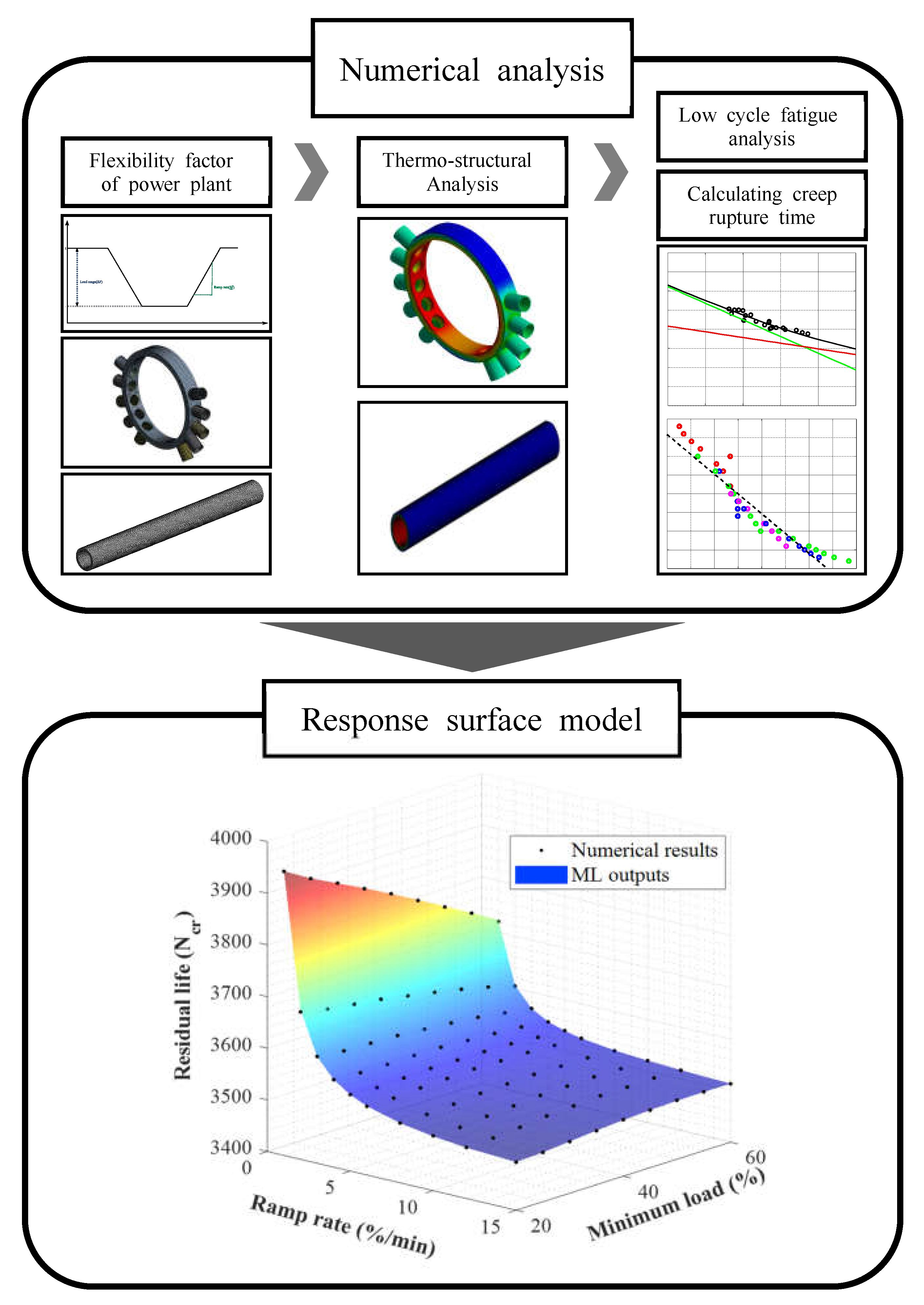
The flowchart for studying the remaining life assessment of high-temperature pipes under flexible driving conditions is as follows. First, we calculated the stresses and strains using the thermo-structural simulation program ANSYS Mechanical. The boundary conditions of FEA were determined by the flexible operation cycle. Second, by utilizing the solutions (i.e., strain and stress range), we numerically evaluated the fatigue and creep damages through the Coffin–Manson equation [17] and the Larson–Miller method [18]. We considered the creep–fatigue interaction, which reduces the service time of the structure. Finally, a response surface model using a machine learning method was developed, which performs life assessment without repetitive experiments or numerical analysis. Our study aimed to estimate the residual life to failure under flexible operating conditions by performing finite element analysis (FEA). First, we calculated the strain range in the high-temperature pipe using thermo-structural analysis. We determined an analytical solution for high-temperature pipes under thermal conditions (i.e., convection, conduction, and radiation) and compared it to the numerical solution to verify our FEA platform. In addition, we evaluated the fatigue life using the Coffin–Manson equation [17] and the life by creep damage through the Larson–Miller method [18] under high pressure and temperature. Considering the creep–fatigue interaction, we calculated the overall damage and residual life of the power plant components. We also analyzed the response to the fatigue life for each variable (i.e., minimum load changes and ramp rate). As a result, we confirmed that creep had a greater effect on the overall life than fatigue, and flexibility significantly affected the creep–fatigue damage and residual life. Furthermore, this study introduced a response surface model using a machine learning method, which performs life assessment without repetitive experiments or numerical analysis.

2. Methodology

2.1. Thermo-Structural Analysis for Evaluation of Strain Range during Flexible Operation

In flexible operation, conventional power from fossil fuels is adjusted to generate power based on daily consumption. Flexibility is a factor that determines how the plant quickly controls the load in response to the changing demand for electricity. To increase the proportion of renewable energy, conventional power plants are required to control the load freely. However, high flexibility (low minimum load, fast ramp rate) causes rapid load changes, resulting in thermal damage to facilities with extreme load variations [19,20]. Therefore, this study investigated the relationship between the flexibility and thermo-mechanical behavior of high-temperature components in power plants.
We considered two main factors: ramp rate and minimum load. The ramp rate is the loading rate during flexible operation. A plant with a high ramp rate can rapidly respond to operating conditions. The minimum load is the lowest power that can be stably applied. The generation characteristics of the plant are more flexible with a lower minimum load. It is challenging to thoroughly analyze an actual situation because complex load fluctuations caused by natural phenomena should be considered. This focused on the tendency of the components to fail, thus simplifying the analysis. Despite the deviation from reality, this model proved sufficient for identifying the failure tendency. Figure 1 shows the ideal flexible operation cycle, divided into the following four sections.
The analysis was conducted for the flexible operation cycle presented in Figure 1, and the temperature and pressure of the working fluid varied according to the power generation output that changed from (a) to (d). This high-temperature steam applies a thermo-structural load to the header components and pipes. The FEA was performed with these components under ideal flexible operating conditions. The structure of the entire power plant was too complex and large to perform numerical analysis. As a result, we substituted the model with one column of header and piping by sub-modeling [9,21]. Plant facilities are subjected to loads by high-temperature fluids. Therefore, they are influenced by the hydrodynamics of their flows. However, the flow patterns of the fluids were not important in this study because we aimed to evaluate the structural behavior of high-temperature components under thermal conditions. Thus, we assumed that the flow field around the analysis model was sufficiently large and that the local temperature and heat transfer coefficient were equal to the empirically obtained average values [22,23].
Figure 2 presents a flowchart of the analysis. First, we derived the boundary conditions for the heat and internal pressure of each structural element based on heat transfer theories and solid mechanics. Equation (1) expresses the differential heat conduction in cylindrical coordinates and Equation (2) expresses the triaxial strain formula with the thermal effects.
1 r r ( r k T r ) + 1 r 2 ϕ ( k T ϕ ) + z ( k T z ) + e ˙ g e n = ρ c T t
ε t = 1 E { σ t ν ( σ r + σ z ) } + α T ε r = 1 E { σ r ν ( σ t + σ z ) } + α T ε z = 1 E { σ z ν ( σ t + σ r ) } + α T
where ρ , c , T , E , e ˙ g e n corresponds to the density, specific heat, temperature, elastic modulus, and heat generation, respectively. ε t , ε r , ε z indicate the hoop, radial, and axial strains, respectively. Finally, σ t , σ r , σ z represent the hoop, radial, and axial stresses.
Then, we calculated the stresses using the thermo-structural simulation program ANSYS Mechanical. The coupling analysis resolved the strain range problem corresponding to each condition. Additionally, utilizing the solution, we numerically evaluated the creep and fatigue damages using MATLAB (See Section 3.1 and Section 3.2). Finally, we considered the creep–fatigue interaction, which reduces the service time of the structure. Our model applied the condition in the creep–fatigue envelope corresponding to the ASME boiler section. The residual life of an object was evaluated by determining whether the structure was broken when it exceeded the threshold.

2.2. Creep–Fatigue Damage Theory

Thermo-structural loads can damage power plant components in the form of creep or fatigue. The fatigue life of the components is primarily evaluated using the Coffin–Manson model and low-cycle fatigue life equation [17].
ε 2 = σ f E ( 2 N f ) b + ε f ( 2 N f ) c
In Equation (3), ε is the strain range and N f is the critical cycle for fatigue failure. σ f = 807 MPa and b = − 0.1486 are the coefficients and exponents for elastic deformation, and ε f = 0.1125 and c = − 0.4355 the ones for plastic deformation, respectively. These are material constants derived from fatigue test results [24]. Additionally, in the high-stress range, the alternating load generates a high mean stress σ m , and derives a mean stress effect that further reduces the fatigue life [25,26]. In this paper, the fatigue life was predicted using Morrow’s equation (Equation (4)), considering the mean stress effect in the strain-life approach [27].
ε 2 = σ f E ( 1 σ m σ f ) ( 2 N f ) b + ε f ( 2 N f ) c
Palmgren [28] and Miner [29] defined pure fatigue damage as the sum of the ratio of the progressive cycle N to the failure cycle N f , as expressed by Equation (5). The fatigue damage is a time-independent variable because N f follows the Morrow equation and depends only on the load change.
D f = i N N f
The creep deformation should also be considered in the design of thermal power plants, as they are exposed to high temperatures for an extended period while operating. The creep rupture time depended on the stress and temperature applied to the model, and the relationship could be determined experimentally. The National Institute of Material Science (NIMS) conducted creep tests at various stresses and temperatures on the SUS304 steel [30]. Several studies have employed the Larson–Miller method to predict creep life by defining the Larson–Miller parameter (LMP) using Equation (6) [18,31]. According to the experimental data, the stress was linearly proportional to LMP, as expressed in Equation (6). The coefficients A = −64.3 and B = 1474 are obtained by solving a least-squares problem.
σ r = A × ( L M P ) + B w h e r e L M P = T log 10 t r + 20
Similar to fatigue damage, creep damage can be calculated using the cumulative damage model. Robinson defined creep damage as the ratio of the loading time t to the rupture time t r at a specific stress and temperature, as expressed in Equation (7) [32]. In other words, the rupture time can be predicted from the stress and temperature conditions using Equation (6), and the creep damage was evaluated using the following formula:
D c = i t t r
Equation (8) summarizes the creep–fatigue damage interaction. When the cumulative damage D exceeded the permissible damage value D a , the material was considered to have failed [33]. The simplest rule for evaluating creep–fatigue damage is the linear damage summation rule, which sets D a to 1 [18]. The D a value can be defined empirically, depending on the load type and material properties [34].
D = D f + D c D f + D c < D a
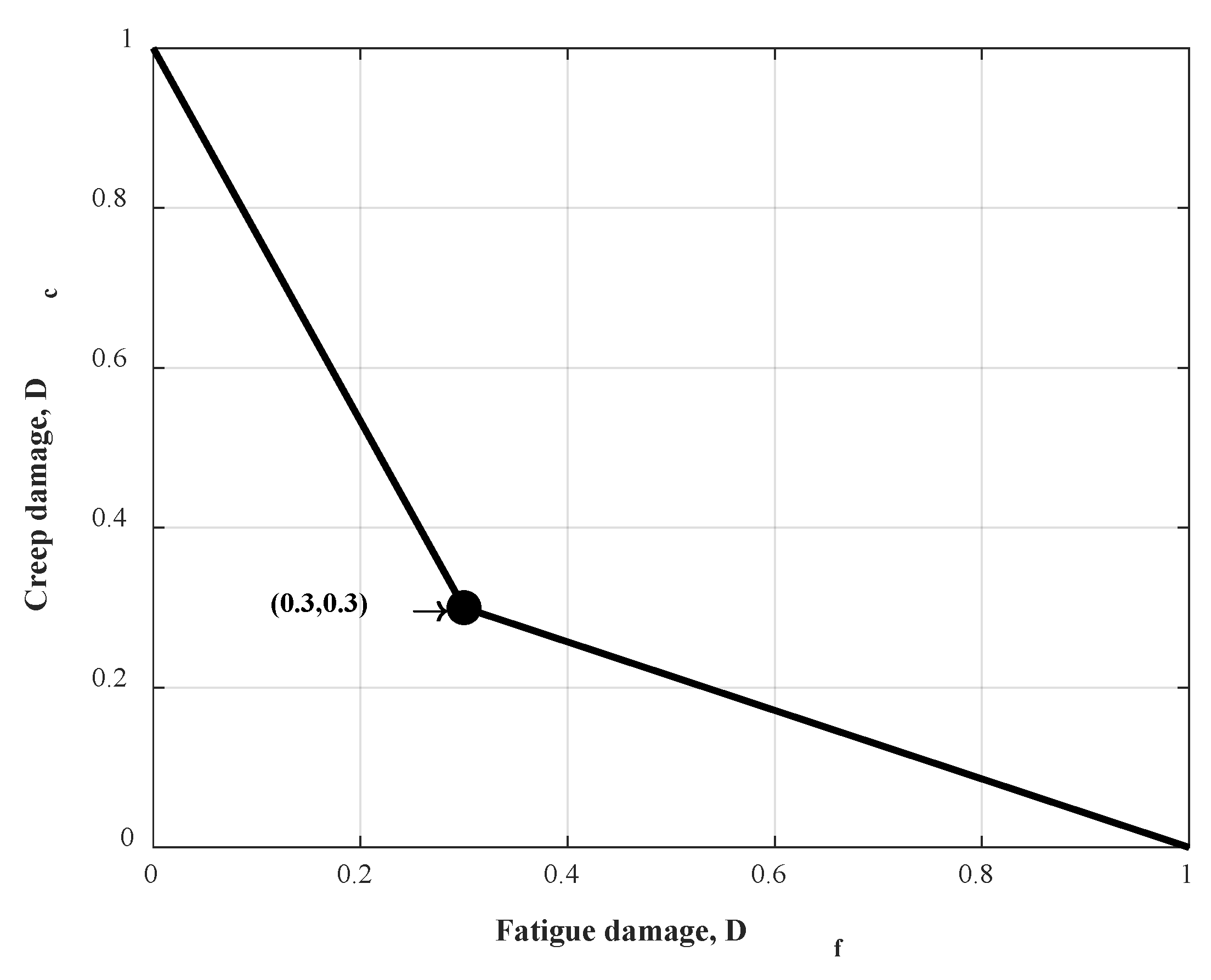
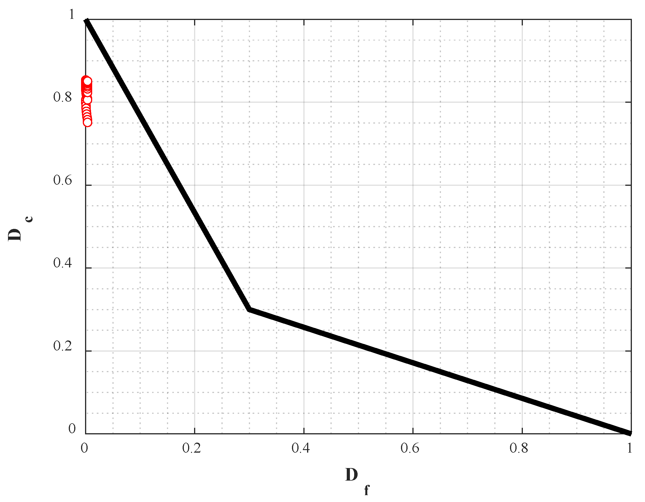
A conservative safety factor should be considered during the design stage to avoid unintentional power plant destruction. Therefore, the damage model for objects should be applied conservatively, which involves a higher safety factor. Figure 3 shows the ASME standard design of SUS304 obtained through experiments, which has a joint at (0.3, 0.3). In the bilinear region of ASME Section III for boilers and pressure vessels, D c and D f follow the two relational expressions in Equation (9) [35]. The critical cycle for safe operation under flexible conditions was estimated by solving these two inequalities.
D c 7 3 D f + 1 f o r   D f 0.3 D c 3 7 ( D f 1 )   f o r   D f 0.3

2.3. Machine Learning Techniques

We derived the residual life from a specified set of flexibility factors through experiments or computational analyses. However, obtaining all outputs for the entire flexibility range using only the aforementioned methods is time consuming and inefficient. Therefore, this study entailed the development of a life assessment method that employs machine learning to predict the life for operating conditions that have not been previously analyzed.

2.3.1. Feedforward Neural Network Model

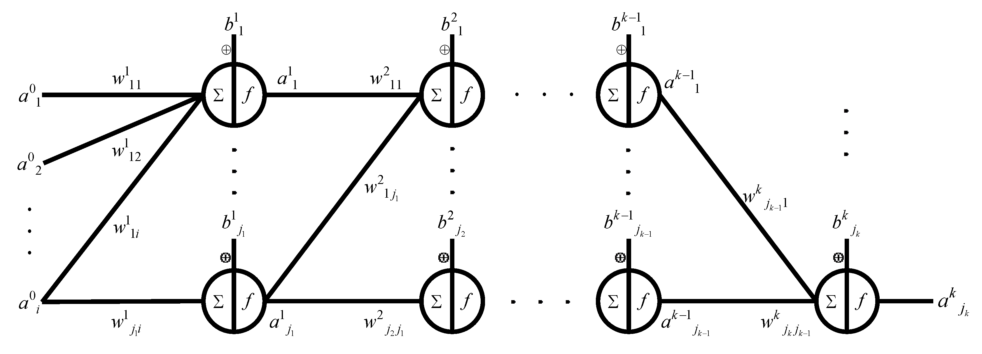
The feedforward neural network is an artificial neural network (ANN) model that propagates information from the input layer to the output layer. In this network, each hidden layer uses a rectified linear unit (ReLU) function, f ( x ) max ( 0 , x ) , as an activation function to provide the learning data. The j t h node value of the k t h hidden layer was given by Equation (10), and the model was trained to reduce the mean-squared error between the data and actual output. The upper subscript k corresponds to the label number of the layer, the lower subscript j to the label of the recipient node, and i to the label of the giver node. Let n l a y e r be the number of hidden layers; then, a i 0 is the input value of the i t h node, and a i n l a y e r + 1 is the output value of the i t h node.
a j k = f ( b j k + i = 0 j k 1 w j i k a i k 1 )
The ANN model in Figure 4 is trained using a back-propagation algorithm called Bayesian Regularization. The letter updates the weights w j i k and bias b j k using the partial differentiation of the objective function V ( x ) . The algorithm computes x = [ J T ( x ) J ( x ) + μ I ] 1 J T ( x ) e ( x ) to update the V ( x ) to V ( x + x ) . This process continues until V ( x ) reaches the optimal value [36]. In the Bayesian Regularization algorithm, V ( x ) consists of a linear combination of the sum of square errors e ( x ) 2 and the sum of square weights w ( x ) 2 , where a α and a β are adjusted through Bayesian optimization [37]:
V B R ( x ) = a α e ( x ) 2 + a β w ( x ) 2 V B R
e ( x ) 2 = ( t ( x ) a n l a y e r + 1 i ) 2

2.3.2. Hyperparameter Optimization Using Random Search

To improve the performance of the machine learning model, the hyperparameters (e.g., learning rate and number of hidden layers) should be appropriately selected through an empirical method, such as a grid search or random search. The grid search algorithm discretizes the range of hyperparameter values into a finite set, or grid of values and trains the ANN model multiple times. The number of training trials is N = k n k , where n k refers to the number of grid values of the k t h hyperparameter. A grid search performs well in low-dimensional problems, but its exhaustive strategy necessitates a large number of trials when there are numerous hyperparameters. For example, in a test including hyperparameters with 10 discrete values, a grid search will require 10 4 trials to identify the best performing value.
The random search algorithm overcomes this difficulty. It generates random combinations of values from a given hyperparameter range and selects the combination set with the best performance. When tuning multiple hyperparameters, it is more likely to find the optimal value than the grid search. Furthermore, more time is reserved when determining the optimal parameters to use for training the machine learning model [38]. Numerous studies have demonstrated the algorithm’s accuracy through statistical and mathematical approaches [38,39,40]. Figure 5 shows a schematic comparison of the two search methods. Under the same conditions, the random search method offers better accuracy if the performance responses are too complex or sensitive to specific hyperparameters.

3. Numerical Examples

3.1. Validation for Thermo-Structural FE Model

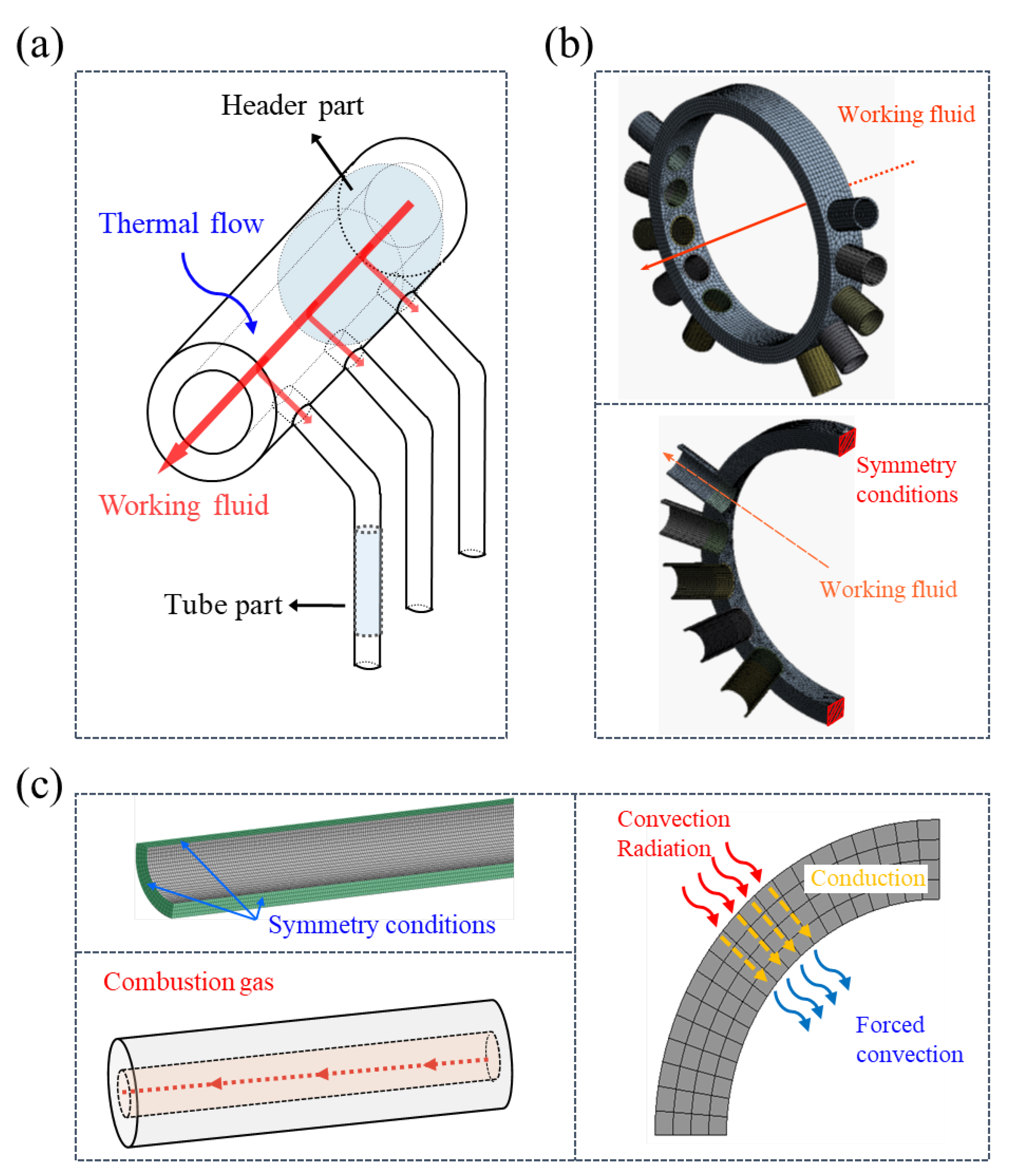
We used the ANSYS Workbench software 2022 R2 for thermo-structural analysis. Numerical results were compared to the analytical solution to validate the analytical method. Heat transfer from the combustion gas and work fluid occurs during the boiler operation. The combustion gas interacts with the outer walls of the pipe components through natural convection and radiation. In addition, the working fluid flowing inside the pipe transfers heat to the inner wall through forced convection. The header part, located outside the combustion chamber, was not affected by the combustion gas and was under standard air conditions. The overall boundary conditions of the header and tube components are shown in Figure 6. Power plants are vulnerable to creep and fatigue failure. To this end we used Creep Strength Enhanced Ferritic Steel (CSEF) in this environment, which exhibits good heat resistance, and high creep strength. In this study, we used SUS304 steel, a common type of CSEF steel. Table 1 lists the composition of the SUS304 steel. The temperature conditions change as the load fluctuates, owing to flexible operation. Therefore, the material properties of SUS304 are temperature dependent, and the temperature variation due to the operating conditions affects the properties. Table 2 and Table 3 list the material properties and thermo-structural boundary conditions with the load level. The values between these categories were interpolated linearly.
Equation (12.a) defines the heat transfer coefficient ( h ) as the product of the thermal conductivity k and the Nusselt number ( N u ). N u is related to the Reynolds ( Re = ρ V D / μ ), Rayleigh ( Ra = g α ν φ ( T s T ) D 3 ), and Prandtl numbers ( Pr = λ / φ ), where μ is the viscosity, φ is the thermal diffusivity, λ is the kinematic viscosity, V is the flow velocity, D is the diameter of the pipe, and g is the acceleration due to gravity. Equation (12.b) shows the empirical formulas used to define N u [23,41]. Given the value of N u , the heat transfer coefficient can be calculated from Equation (12.a) [41].
h = N u × k
Nu = 0.023 Re 0.5 Pr 0.4                                       f o r   F o r c e d   c o n v e c t i o n 0.6 + 0.387 Ra 1 + 0.559 Pr 9 / 16 16 / 9 1 / 6 2 f o r   N a t u r a l   c o n v e c t i o n
Stefan–Boltzmann’s law was used to calculate the radiant heat transfer coefficient h r a d of the combustion gas (see Equation (13)), where σ is the Stefan—Boltzmann constant, ε t o t is the total emissivity, T g is the gas temperature, and T w is the wall temperature adjacent to the gas [42]. The composition and properties of the combustion gas mixture are described in the literature [43,44].
q = h r a d ( T g T w ) = σ ε t o t ( T g 4 T w 4 ) w h e r e   h r a d = σ ε t o t T g 4 T w 4 T g T w , ε t o t = ( 1 + ε t u b e ) 2 ε g a s
Equation (1) provides a solution for the heat conduction equation. It is difficult to verify this model for header components with complex geometries. Therefore, this study validated the model by comparing these equations with the numerical results of a simple straight-pipe model. The boundary conditions used in the analysis are shown in Figure 6. This can be summarized as follows:
(a)
Radiant and convective heat transfer from combustion gas at the outer wall;
(b)
Conduction in the tube wall;
(c)
Convection at the inner wall of the working fluid.
The tube temperature changed from (a) to (b), and thermal deformation occurred. The heat flux during the heat transfer process is explained in the literature [23]. As each heat flux q ˙ is equal throughout the entire section, the heat flux at any time step follows Equation (14), which is a quaternary equation for heat flux. Therefore, we used Newton’s method to solve the complicated equation and derive its approximate solution, which was compared to the numerical solution calculated from the FE model. The validation was performed in the load-descending section, as shown in Figure 1b.
q ˙ = T . e x T . i n + ε t o t σ { T . e x ( q ˙ ( R c o n d R c o n d . i n ) + T . i n ) 4 } × R c o n v . e x R c o n d + R c o n v . i n + R c o n v . e x
T . e x and T , i n are the external and internal temperatures of the tube, respectively, R c o n d is the thermal conductivity k divided by the thickness D , R c o n v , e x and R c o n v , i n are the reciprocal of the convective film coefficients h e x and h i n , which follow Equations (12) and (13), respectively.
Figure 7 compares the analytical solutions using Equation (14) and numerical results. The right-hand side of Equation (1) can be solved by utilizing the approximate equality between the heat flux and temperature over time. Using a finite difference method, changes in temperature with location can also be computed, in agreement with the laws of physics [23]. Therefore, the thermal boundary condition of the numerical model is well posed.
Temperature variations cause thermal deformation and stress in the object. Their mechanical behavior follows Equation (2). The triaxial thermal stresses of the superheater tube in a cylindrical coordinate system follow Equation (15) [22].
σ r = E α 1 ν 1 r 2 r 2 r i 2 r o 2 r i 2 r i r o T r   d r r i r T r   d r R a d i a l   s t r e s s σ t = E α 1 ν 1 r 2 r 2 + r i 2 r o 2 r i 2 r i r o T r   d r + r i r T r   d r T r 2 H o o p   s t r e s s σ z = E α 1 ν 1 r 2 2 r o 2 r i 2 r i r o T r   d r T A x i a l   s t r e s s
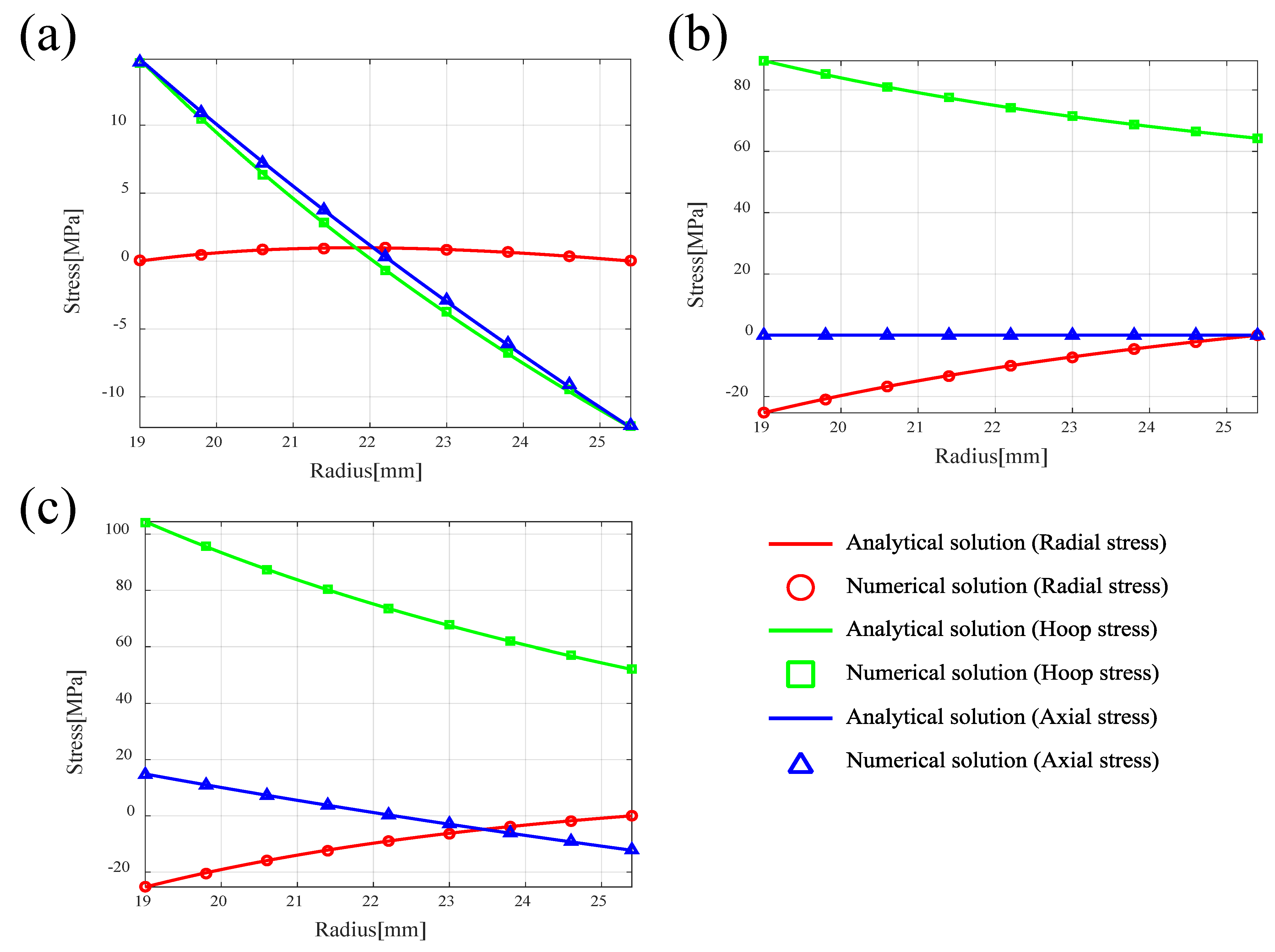
From the numerical model, the thermal stress was estimated and compared with the analytical solution, as shown in Figure 8. Figure 8a compares the thermal results, confirming that the heat transfer and thermal load conditions in the numerical model follow the governing equation. In addition, the power plant equipment is subjected to internal pressure. Dowling [45] proposed stresses in thick-walled pressure vessels by internal pressure p (see Equation (16)).
σ r = p r i 2 r o 2 r i 2 r o 2 r 2 1       R a d i a l   s t r e s s σ t = p r i 2 r o 2 r i 2 r o 2 r 2 + 1     H o o p   s t r e s s σ z = 0 A x i a l   s t r e s s
The comparison of stress in the superheater tube under the structural load by pressure is presented in Figure 8b. Equations (15) and (16) can be linearly combined using the superposition method, as the stress generated by the heat and pressure is within the elastic range. Finally, Figure 8c shows the results of the coupled thermo-structural stresses by thermal loading and internal pressure. We validated the boundary conditions of the numerical model by comparing the results to those of the analytical solution.

3.2. Estimation of Fatigue Life under Cyclic Thermal Loads

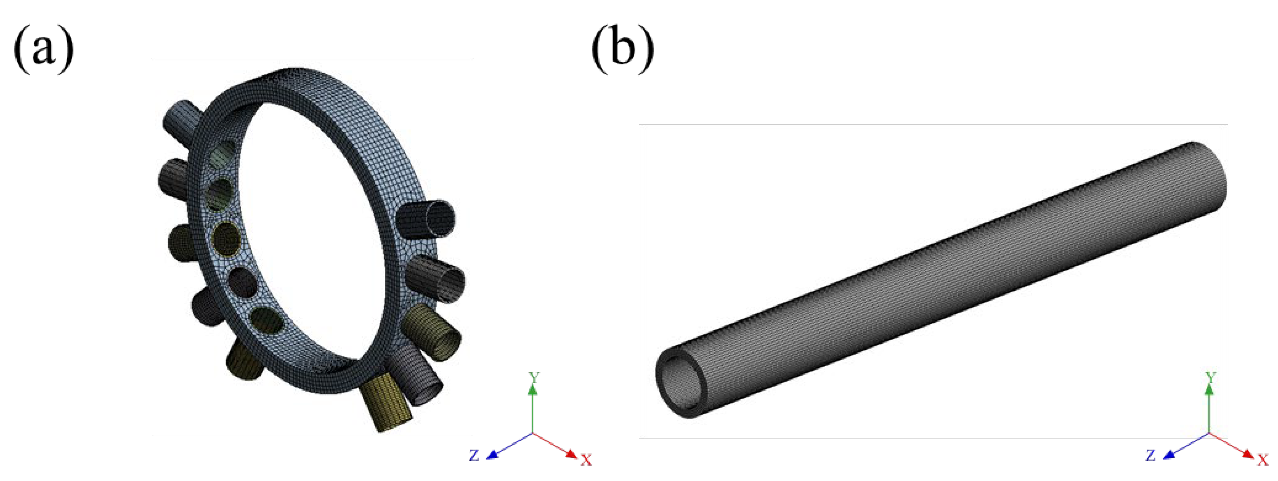
In this analysis, all power plant components were divided into several submodels for time efficiency. Figure 9 shows the numerical models for each part. The finite element model of the components consist of SOLID 185 3D elements, which are linear hexahedral elements used for thermo-structural analysis. Table 4 lists the number of elements and nodes [46].
The thermo-structural boundary conditions are changed, since the factors of flexible operation modify the power level of the power plant. Each feature depends on the time t and the power generation output ϕ ( t ) at any given moment. Any boundary condition X (e.g., the temperature of the working fluid and internal pressure at that time) follows Equation (17), where X and ϕ represent the changes in the boundary condition and power generation over time in a specific operation section, respectively. Additionally, X o and ϕ o indicate the initial values.
X ( t ) = X ϕ ϕ ( t ) ϕ o + X o
The electricity power level ϕ ( t ) affects the condition X . Furthermore, it varied depending on the position in the boiler tube. Therefore, they are path dependent, and X follows the binary function of Equation (18). The distance d is d i n at the inlet and d o u t at the outlet of the path.
X ( d , t ) = X ( d o u t , t ) X ( d i n , t ) d o u t d i n d d i n + X ( d i n , t )
Figure 10 shows the numerical contours of the boiler parts, where the boundary conditions of Equation (18) were applied under a minimum load of 20% and a ramp rate of 3%/min. Table 5 summarizes the stress and temperature results of the reheater header and superheater tube. The creep–fatigue damage in Equation (6) depends on the data listed in Table 5. The maximum stress in the header part was 1.92 times higher than that in the tube part. Therefore, we expected the header component to be more damaged by the thermo-structural load than the other parts. Based on this result, we determined that this part is vulnerable to creep–fatigue damage and selected it for assessing the residual life.
This section may be divided by subheadings. It should provide a concise and precise description of the experimental results, their interpretation, as well as the experimental conclusions that can be drawn.

3.3. Creep and Fatigue Life of the Header

The creep–fatigue damage of the header in Equation (7) depends on the change in flexibility during the operation. We assumed that the power plant had an ideal flexible operation cycle, as shown in Figure 1, and that the holding time of the minimum load section was t c = 3 h . Under these assumptions, the operating time in each section is defined as t a = 24 ( t b + t c + t d ) ,   t b = t d = P max P min ν ,   t c = 3 , where P min is the minimum load and ν = d P / d t is the ramp rate The creep–fatigue damage was estimated under operating conditions using the data presented in Table 5. Fatigue damage occurred only in sections (b) and (d) of the optimized cycle shown in Figure 1, where the load alternated and caused strain. In contrast, creep damage, which occurs based on stress and temperature levels, appeared throughout the operation cycle. Equation (19) gives the total creep damage D c and fatigue damage D f , that the header receives after operating N cycles, with one cycle being 24 h . We can rearrange Equation (7) to solve for the operation cycle N , to obtain Equation (20). If N reaches the critical cycle N c r , this inequality satisfies the equal sign, and the damaged object is considered to have failed.
D = D f + D c = N × ( d f + d c )
N N c r = 3 3 d c + 7 d f   for   D f 0 . 3 3 7 d c + 3 d f   for   D f 0 . 3
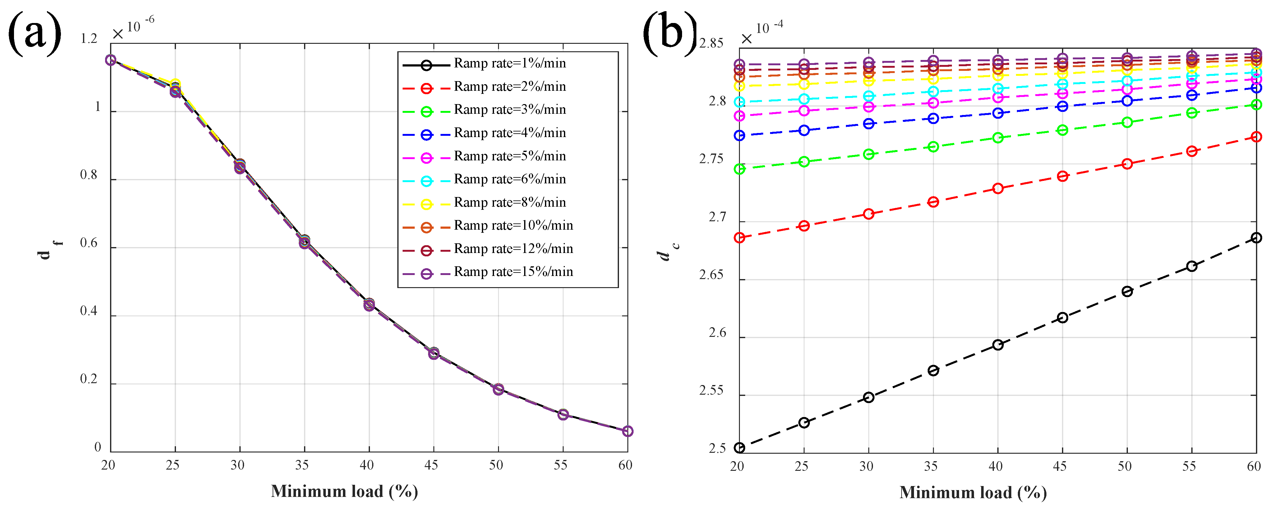
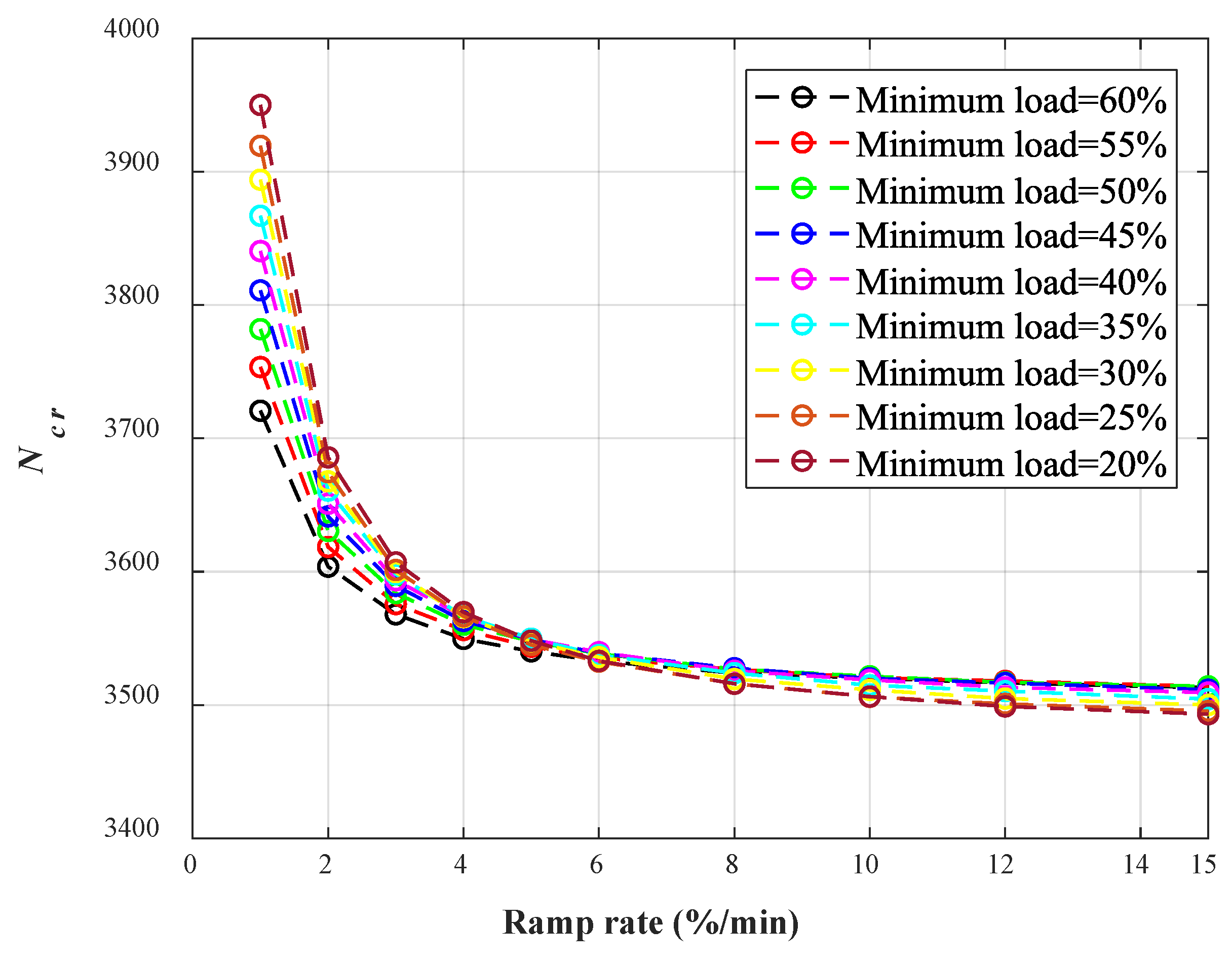
The boundary conditions change when the minimum load changes and affect creep and fatigue damage. The variation in the ramp rate did not affect the conditions, but it affected the operating time, as shown in Figure 1. Since fatigue damage is time independent, it is unaffected by the ramp rate. In contrast, the creep damage varies with the flexibility factor. We estimated the critical cycle for the given creep–fatigue damage using Equation (20), Figure 11a shows the fatigue damage as a function of ramp rate and minimum load change. The results indicate that the fatigue damage was only affected by the variation in the minimum load. The fatigue damage decreased as the minimum load increased and was unaffected by the ramp rate changes. In other words, it is independent of the ramp rate. In contrast, creep damage depends on two flexibility factors (i.e., ramp rate and minimum load), as shown in Figure 11b. We demonstrated that the creep damage was higher for increasing ramp rate and minimum load. Additionally, the creep damage change for the minimum load over a certain ramp rate was not significant. This results from the fact that sections (b) and (d) in Figure 1, which cause fatigue damage, are shortened at high ramp rates, and creep damage becomes dominant.
The creep damage per cycle d c is approximately 100 times higher than the fatigue damage d f in most operating conditions. As a result, the expectancy of the critical cycle N c r is dominated by creep effects (Figure 12). The boiler parts generally have lower residual life under operating conditions that cause high creep damage levels (i.e., higher minimum load and ramp rate). Figure 13 shows the damage to the plant header during 3000 cycles in the creep–fatigue envelope, suggesting that the plant element is vulnerable to creep under most flexibility cases. During the flexible operation of thermal power plants, engineers must prioritize creep damage over fatigue damage.
Although the fatigue damage is minor compared to the creep damage, the effect of fatigue damage may increase as the ramp rate and minimum load decrease. As a result, fatigue damage must be considered when evaluating the residual life. Furthermore, this study assumed that only two load fluctuations (sections (b) and (d) of Figure 1) occurred per day, considering an ideal flexible operation. However, the proportion of fatigue to residual life is expected to increase as more complex operations progress. For these reasons, the fatigue effect should also be considered when assessing the residual life of boiler components.

3.4. Response Surface Model

Τo investigate the residual life, we estimated the parameters (e.g., strain range, temperature, and stress level). We proposed an ANN regression model that predicts the residual life under flexible operating conditions based on the above results. The proposed model follows the neural network structure shown in Figure 4. To improve its accuracy, we selected three hyperparameters for adjustment: the number of hidden layers ( n l a y e r ), the number of nodes per layer ( n n o d e s ), and the initial learning rate ( ζ i n i t a l ). Table 6 lists the ranges of the selected parameters. Twenty parameter sets were randomly extracted using the random search method and the model was trained to find the optimal set of hyperparameters.
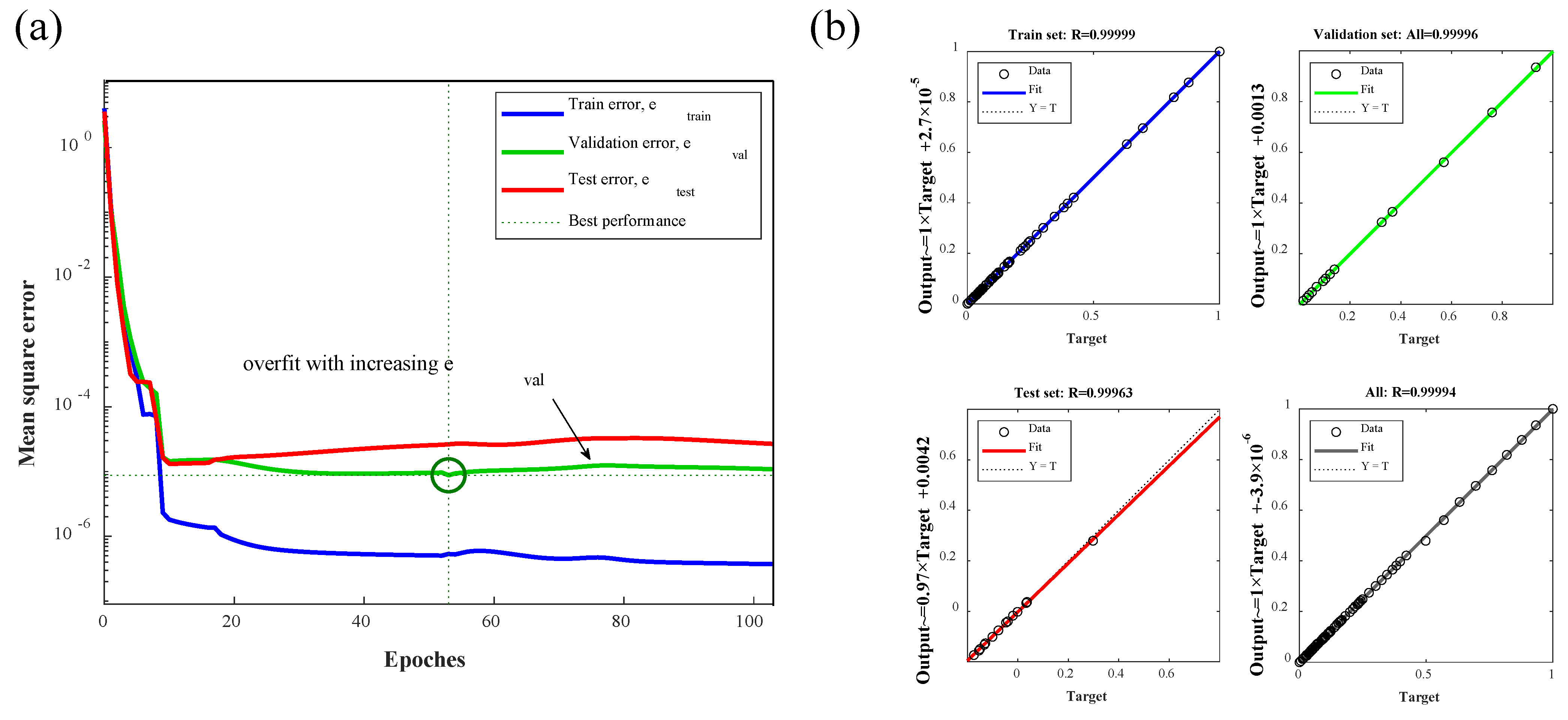
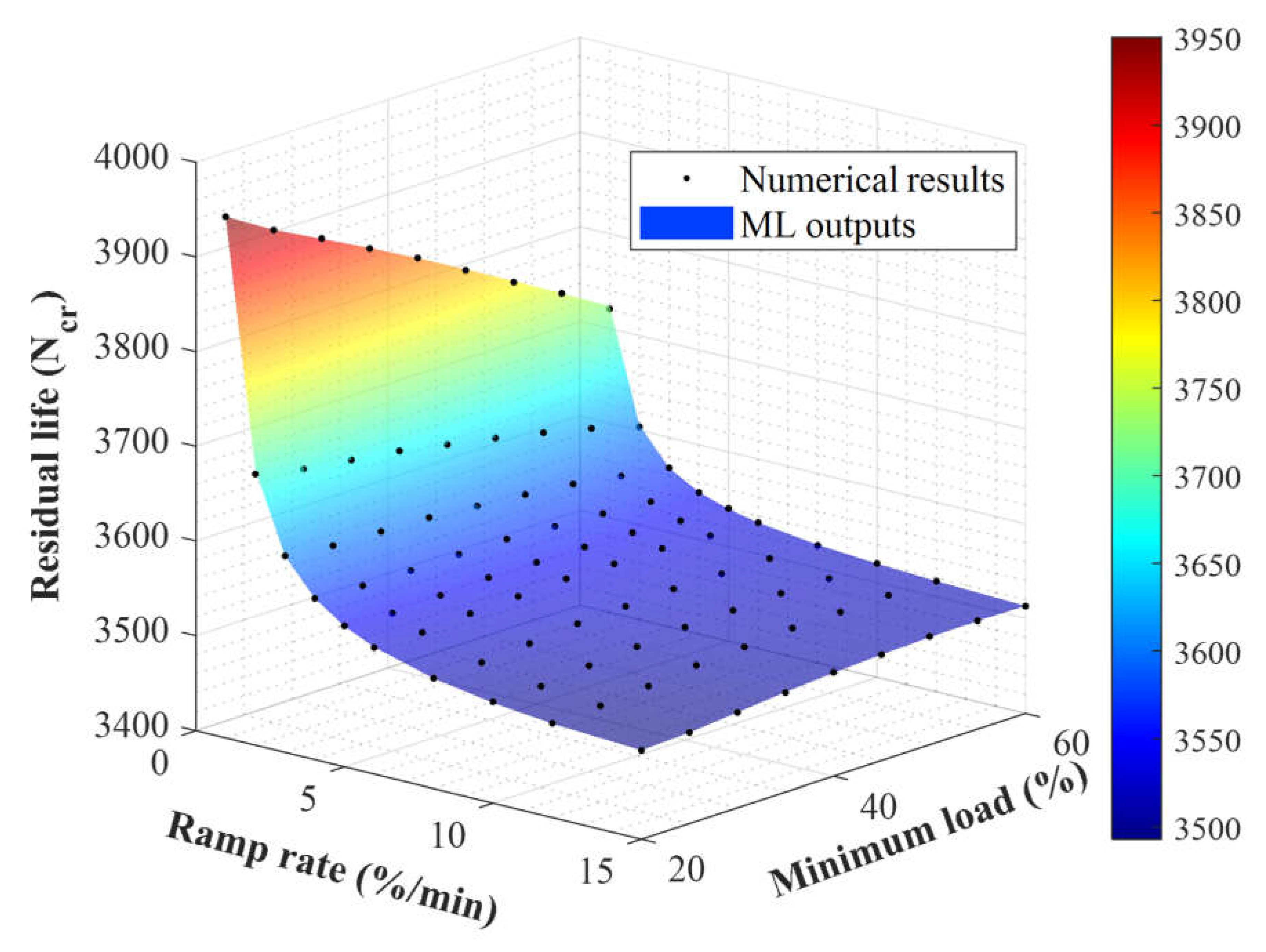
To evaluate the performance of the neural network model, it is essential to normalize the input and output data to share the same scale. We used min–max normalization, which places the smallest value of the data at zero and the largest at one. The other values are scaled between them. Our ANN model sets each flexibility (i.e., ramp rate and minimum load) as an input value and the residual life N c r as an output value. In the training process using Equations (10) and (11), the machine learning network divides the data into the training set (60%), test set (20%), and validation set (20%) to use for cross-validation. For every iteration i , the network is trained using the training set and evaluated using the test set. The training performance was determined by the mean square error (MSE) e t e s t ( i ) of the test set. The weights and biases were updated accordingly to reduce the error. The error e v a l ( i ) of the trained model was also evaluated on the validation set to avoid overfitting the test set. Our study identified the optimizer with the lowest validation error e v a l ( i b e s t ) at the epoch i b e s t and the model performance as the test error e t e s t ( i b e s t ) at this epoch. Subsequently, the ANN model was trained for each hyperparameter set. Among them, ( n l a y e r , n n o d e s , ζ i n i t a l ) = ( 2 , 28 , 0.0931 ) exhibited the best performance, e t e s t ( i b e s t ) = 2.1798 × 10 5 , and was selected as the optimal set. Figure 14 presents the error and coefficient of correlation R for each dataset. Through this process, we defined a well-constructed ANN model exhibiting a small error for most inputs. Figure 15 shows the optimized structure of the ANN model. We propose an ANN model that can effectively evaluate the residual fatigue life within a given minimum load and ramp rate range.

4. Conclusions

This study aimed to assess the residual life during flexible operation using numerical methods and empirical models. We considered two main factors of flexible operation, ramp rate and minimum load, and investigated their effects on residual life. FEA was performed under the given temperature and pressure conditions to estimate the strain range of the superheater tube and reheater header. The finite element results were verified by comparing them to the analytical solution of the straightened tube under thermal load conditions. We estimated the creep–fatigue life of the reheater header under flexible operation factors using finite element modeling and the Coffin–Manson and Larson–Miller models. We numerically demonstrated that fatigue damage occurred owing to thermal cycling and increased with decreasing minimum load and ramp rate. Nevertheless, creep damage was the dominant damage mechanism. This originates from the fact that the thermal cycle is a low cycle that repeats up to twice a day, and creep is the dominant mechanism in terms of overall damage. In addition, by utilizing the ANN model, we proposed a response surface model for evaluating the residual life of the reheater heater, which is the most vulnerable component under flexible operation. This model can predict the residual life of the reheater header according to the flexible operation factors without performing complex thermo-structural analysis and empirical models for fatigue and creep life.
This is the first systematic study to analyze the effect of the flexible operation on the residual life of the tube and header. To evaluate the residual life under flexible operation conditions using experimental methods, there are some difficulties in terms of time and research execution. In this study, to overcome these difficulties, computational mechanics and empirical equations were used as an approach. It additionally presents a model that can predict the residual life using the response surface model. We believe that our findings will aid the efficient operation of thermal power plants by optimizing flexible operation factors in the future. Furthermore, it is expected that this study will contribute to the cost reduction and determination of maintenance cycles in power plant maintenance under flexible driving conditions.

Author Contributions

Conceptualization, J.-H.H. and D.-W.J.; methodology, J.-H.H. and J.H.; software, J.H.; validation, J.H. and M.P.; formal analysis, J.H. and M.P.; investigation, J.H. and M.P.; data curation, J.H. and J.-M.K.; writing—original draft preparation, J.-H.H. and D.-W.J.; writing—review and editing, J.H. and D.-W.J.; visualization, J.H.; supervision, J.-H.H. and D.-W.J.; project administration, J.-H.H. and J.-M.K.; funding acquisition, J.-H.H. All authors have read and agreed to the published version of the manuscript.

Funding

This work was partly supported by the Korea Institute of Energy Technology Evaluation and Planning(KETEP) grant funded by the Korea government(MOTIE) (20224000000220, Jeonbuk Regional Energy Cluster Training of human resources) and the National Research Foundation of Korea (NRF) grant funded by the Korea government (MSIT) (2020R1F1A1060442).

Data Availability Statement

The data obtained from this research are presented in their entirety in this manuscript. If you wish to obtain specific information on the raw data, you may request it directly from the corresponding author.

Conflicts of Interest

The authors declare no conflict of interest.

References

  1. Belbute, J.M.; Pereira, A.M. An alternative reference scenario for global CO2 emissions from fuel consumption: An ARFIMA approach. Econ. Lett. 2015, 136, 108–111. [Google Scholar] [CrossRef]
  2. Alam, M.M.; Murad, M.W.; Noman, A.H.; Ozturk, I. Relationships among carbon emissions, economic growth, energy consumption and population growth: Testing Environmental Kuznets Curve hypothesis for Brazil, China, India and Indonesia. Ecol. Indic. 2016, 70, 466–479. [Google Scholar] [CrossRef]
  3. Hanif, I. Impact of fossil fuels energy consumption, energy policies, and urban sprawl on carbon emissions in East Asia and the Pacific: A panel investigation. Energy Strategy Rev. 2018, 21, 16–24. [Google Scholar] [CrossRef]
  4. Energy-Charts. Average Net Electricity Generation during One Week in Germany 2021. 2021. Available online: https://www.energy-charts.info/ (accessed on 12 December 2022).
  5. Papadopoulou, A.G.; Vasileiou, G.; Flamos, A. A comparison of dispatchable RES technoeconomics: Is there a Niche for concentrated solar power? Energies 2020, 13, 4768. [Google Scholar] [CrossRef]
  6. Alobaid, F.; Mertens, N.; Starkloff, R.; Lanz, T.; Heinze, C.; Epple, B. Progress in dynamic simulation of thermal power plants. Prog. Energy Combust. Sci. 2017, 59, 79–162. [Google Scholar] [CrossRef]
  7. Bethmont, M. Damage and lifetime of fossil power plant components. Mater. High Temp. 1998, 15, 231–238. [Google Scholar] [CrossRef]
  8. Ray, A.; Tiwari, Y.; Sinha, R.; Chaudhuri, S.; Singh, R. Residual life prediction of service exposed main steam pipe of boilers in a thermal power plant. Eng. Fail. Anal. 2000, 7, 359–376. [Google Scholar] [CrossRef]
  9. Roy, H.; Ghosh, D.; Roy, P.; Saha, A.; Shukla, A.K.; Basu, J. Failure investigation of platen superheater outlet header. J. Manuf. Sci. Prod. 2009, 10, 17–24. [Google Scholar] [CrossRef]
  10. Al-Kayiem, H.; Albarody, T. Numerical investigation of superheater tube failure. WIT Trans. Eng. Sci. 2016, 106, 1–10. [Google Scholar]
  11. Li, M.; Benaarbia, A.; Morris, A.; Sun, W. Assessment of potential service-life performance for MarBN steel power plant header under flexible thermomechanical operations. Int. J. Fatigue 2020, 135, 105565. [Google Scholar] [CrossRef]
  12. Okrajni, J. Thermo-mechanical fatigue conditions of power plant components. J. Achiev. Mater. Manuf. Eng. 2009, 33, 53–61. [Google Scholar]
  13. Daga, R.; Samal, M.K. Creep Fatigue Damage Assessment of an In-service Superheater Outlet Header. In Proceedings of the International Conference on Fatigue Durability and Fracture Mechanics, Bangalore, India, 28–30 May 2015. [Google Scholar]
  14. Avagianos, I.; Rakopoulos, D.; Karellas, S.; Kakaras, E. Review of process modeling of solid-fuel thermal power plants for flexible and off-design operation. Energies 2020, 13, 6587. [Google Scholar] [CrossRef]
  15. Ali, U.; Akram, M.; Font-Palma, C.; Ingham, D.B.; Pourkashanian, M. Part-load performance of direct-firing and co-firing of coal and biomass in a power generation system integrated with a CO2 capture and compression system. Fuel 2017, 210, 873–884. [Google Scholar] [CrossRef]
  16. Haryanto, A.; Hong, K.-S. Modeling and simulation of an oxy-fuel combustion boiler system with flue gas recirculation. Comput. Chem. Eng. 2011, 35, 25–40. [Google Scholar] [CrossRef]
  17. Shuaeib, F.; Benyounis, K.; Hashmi, M. Material Behavior and Performance in Environments of Extreme Pressure and Temperatures; Elsevier: Amsterdam, The Netherlands, 2017. [Google Scholar]
  18. Goyal, S.; Mariappan, K.; Shankar, V.; Sandhya, R.; Laha, K.; Bhaduri, A. Studies on creep-fatigue interaction behaviour of Alloy 617M. Mater. Sci. Eng. A 2018, 730, 16–23. [Google Scholar] [CrossRef]
  19. Bauerbach, K.; Grammenoudis, P. Fundamental considerations of the effects of flexible operation on the fatigue of power plant components. Mater. High Temp. 2021, 38, 252–261. [Google Scholar] [CrossRef]
  20. Impram, S.; Nese, S.V.; Oral, B. Challenges of renewable energy penetration on power system flexibility: A survey. Energy Strategy Rev. 2020, 31, 100539. [Google Scholar] [CrossRef]
  21. Farragher, T.; Scully, S.; O’Dowd, N.; Leen, S. Development of life assessment procedures for power plant headers operated under flexible loading scenarios. Int. J. Fatigue 2013, 49, 50–61. [Google Scholar] [CrossRef]
  22. Kandil, A.; El-Kady, A.; El-Kafrawy, A. Transient thermal stress analysis of thick-walled cylinders. Int. J. Mech. Sci. 1995, 37, 721–732. [Google Scholar] [CrossRef]
  23. Incropera, F.P.; DeWitt, D.P.; Bergman, T.L.; Lavine, A.S. Fundamentals of Heat and Mass Transfer; Wiley: New York, NY, USA, 1996; Volume 6. [Google Scholar]
  24. Yoshiyuki, F.; Hideaki, N.; Hisashi, H.; Nobuo, N.; Etsuo, T. Data Sheets On Elevated-Temperature, Time-Dependent Low-Cycle Fatigue Properties Of Sus304-Hp (18cr-8ni) Hot Rolled Stainless Steel Plate. National Institute for Materials Science: Tsubaka, Japan, 1985. [Google Scholar]
  25. Xia, Z.; Kujawski, D.; Ellyin, F. Effect of mean stress and ratcheting strain on fatigue life of steel. Int. J. Fatigue 1996, 18, 335–341. [Google Scholar] [CrossRef]
  26. Nihei, M.; Heuler, P.; Boller, C.; Seeger, T. Evaluation of mean stress effect on fatigue life by use of damage parameters. Int. J. Fatigue 1986, 8, 119–126. [Google Scholar] [CrossRef]
  27. Dowling, N. Mean stress effects in strain–life fatigue. Fatigue Fract. Eng. Mater. Struct. 2009, 32, 1004–1019. [Google Scholar] [CrossRef]
  28. Palmgren, A. Ball and Roller Bearing Engineering; SKF Industries Inc.: Philadelphia, PA, USA, 1959. [Google Scholar]
  29. Miner, M.A. Cumulative damage in fatigue. ASME J. Appl. Mech. 1945, 3, A159–A164. [Google Scholar] [CrossRef]
  30. Sawada, K.; Kimura, K.; Abe, F.; Taniuchi, Y.; Sekido, K.; Nojima, T.; Ohba, T.; Kushima, H.; Miyazaki, H.; Hong, H.; et al. Data Sheets on the Elevated-Temperature Properties of 18cr-9ni-3cu-nb-n Stainless Steel Tube for Power Boilers (KA-SUS 304 J1 HTB); National Institute for Materials Science: Tsubaka, Japan, 2018. [Google Scholar]
  31. Song, L.-K.; Bai, G.-C. Multi-surrogate collaboration approach for creep-fatigue reliability assessment of turbine rotor. IEEE Access 2020, 8, 39861–39874. [Google Scholar] [CrossRef]
  32. Robinson, E. Effect of temperature variation on the creep strength of steels. Trans. ASME 1938, 60, 253–259. [Google Scholar] [CrossRef]
  33. Taira, S. Lifetime of structures subjected to varying load and temperature. In Creep in Structures: Colloquium Held at Stanford University, California 11–15 July 1960; Springer: Berlin/Heidelberg, Germany, 1962. [Google Scholar]
  34. Rodriguez, P.; Mannan, S.; Rao, K.B.S. Life prediction methods for creep-fatigue conditions. Trans. Indian Inst. Met. 1987, 42, 25–43. [Google Scholar]
  35. Jetter, R.; Rao, K. Subsection nh-Class 1 Components in Elevated Temperature Service; American Society of Mechanical Engineers: New York, NY, USA, 2002; pp. 369–404. [Google Scholar]
  36. Hagan, M.T.; Menhaj, M.B. Training feedforward networks with the Marquardt algorithm. IEEE Trans. Neural Netw. 1994, 5, 989–993. [Google Scholar] [CrossRef]
  37. Foresee, F.D.; Hagan, M.T. Gauss-Newton approximation to Bayesian learning. In Proceedings of the International Conference on Neural Networks (ICNN’97), Houston, TX, USA, 9–12 June 1997. [Google Scholar]
  38. Bergstra, J.; Bengio, Y. Random search for hyper-parameter optimization. J. Mach. Learn. Res. 2012, 13. [Google Scholar]
  39. Andradóttir, S. An overview of simulation optimization via random search. Handb. Oper. Res. Manag. Sci. 2006, 13, 617–631. [Google Scholar]
  40. Karnopp, D.C. Random search techniques for optimization problems. Automatica 1963, 1, 111–121. [Google Scholar] [CrossRef]
  41. Churchill, S.W.; Chu, H.H. Correlating equations for laminar and turbulent free convection from a vertical plate. Int. J. Heat Mass Transf. 1975, 18, 1323–1329. [Google Scholar] [CrossRef]
  42. Taler, D.; Taler, J. Simplified analysis of radiation heat exchange in boiler superheaters. Heat Transf. Eng. 2009, 30, 661–669. [Google Scholar] [CrossRef]
  43. Otsuka, N. Fireside corrosion. Shreir’s Corros. 2010, 1, 457–481. [Google Scholar]
  44. Cengel, Y.A.; Boles, M.A.; Kanoğlu, M. Thermodynamics: An Engineering Approach; McGraw-Hill: New York, NY, USA, 2011; Volume 5. [Google Scholar]
  45. Dowling, N.E. Mechanical Behavior of Materials: Engineering Methods for Deformation, Fracture, and Fatigue–International Edition; Pearson: London, UK, 2013. [Google Scholar]
  46. Klaus-Jürgen, B. Finite Element Procedures in Engineering Analysis; Prentice-Hall, Inc.: Englewood Cliffs, NJ, USA, 1982; Volume 7632. [Google Scholar]
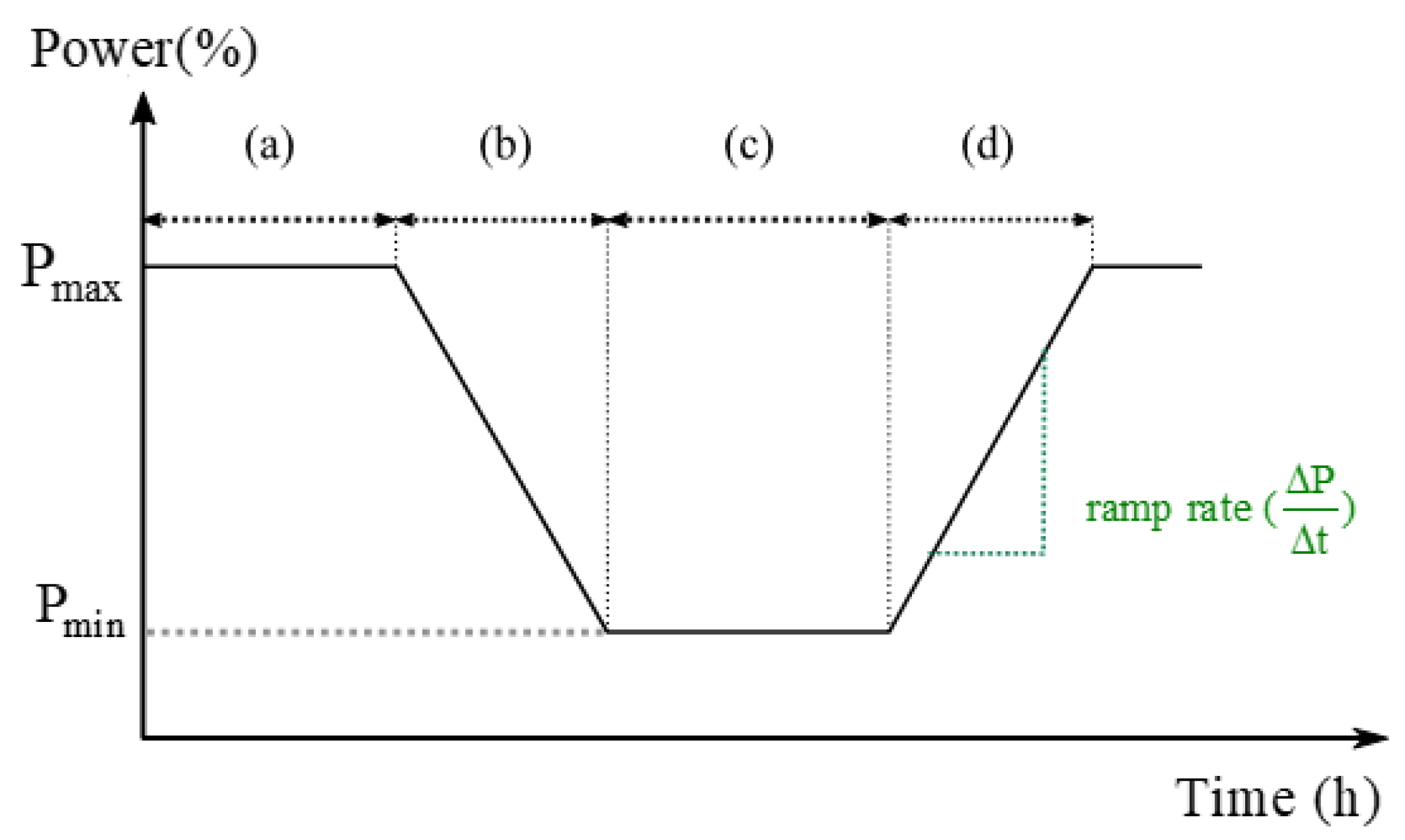
Figure 1. Schematic diagram of the flexible operation cycle. (a) General load operation section: the section where the power plant operates while maintaining the general load ( P max ). (b) Load-decreasing section: the flexible operating section adjusts power in response to an increasing proportion of RES. (c) Minimum load operation section: the section that maintains the minimum load ( P min ). (d) Load increasing section: the section increasing the load from P min to P max .
Processes 11 01679 g001
Figure 2. Flowchart of the entire analysis process.
Processes 11 01679 g002
Figure 3. ASME Section III specification of the bilinear creep–fatigue interaction model.
Processes 11 01679 g003
Figure 4. Schematic diagram of feedforward neural network model.
Processes 11 01679 g004
Figure 5. Comparison of grid search and random search.
Processes 11 01679 g005
Figure 6. (a) Schematic diagram of boundary conditions of the power plant. Thermal conditions for (b) the header component, and (c) tube component.
Processes 11 01679 g006
Figure 7. Validation of heat transfer analysis by comparing the analytical solutions with numerical solutions of (a) wall temperature and (b) heat flux in the power descending section.
Processes 11 01679 g007
Figure 8. Comparison of numerical solution with the analytic solution under (a) thermal, (b) structural, and (c) thermo−structural condition.
Processes 11 01679 g008
Figure 9. Numerical modeling of (a) reheater header and (b) superheater tube component.
Processes 11 01679 g009
Figure 10. Results of the thermo-structural analysis. The temperature of (a) the reheater header and (b) the superheater tube. The stress of (c) the header and (d) the tube.
Processes 11 01679 g010
Figure 11. Damage versus minimum load for (a) fatigue and (b) creep.
Processes 11 01679 g011
Figure 12. Critical cycle with respect to ramp rate.
Processes 11 01679 g012
Figure 13. Creep–fatigue envelop with damage accumulation after 3000 cycles. The red circle represents the cumulative damage of creep and fatigue that occurred after 3000 cycles for the plant header.
Processes 11 01679 g013
Figure 14. Performance of the ANN model. (a) Epoch versus error graph, and (b) regression results with coefficient of correlation R.
Processes 11 01679 g014
Figure 15. Response surface model for entire flexibility boundary.
Processes 11 01679 g015
Table 1. Composition of the SUS304 steel.
ElementsCMnSiCrNiNNbP
Composition (wt%)0.07–0.131.000.01017.0–19.07.5–10.50.05–0.120.30–0.600.040
Table 2. Temperature-dependent properties of the SUS304 steel.
Material PropertyValue at 300 °CValue at 500 °CValue at 700 °C
Density, ρ ( k g / m 3 )779077007610
Thermal expansion coefficient, α ( × 10 6 / ° C ) 9.710.0510.3
Elastic modulus E ( G P a ) 164.78148.93132.38
Poisson’s ratio ν0.28740.29460.3018
Thermal conductivity, k ( W / m   ° C ) 21.46124.92330.98
Specific heat, c ( J / k g   ° C ) 542.62579.71616.81
Table 3. Thermo-structural boundary conditions during the operation of the power plant.
Boundary ConditionUnder 100% ConditionUnder 30% Condition
Tube Steam   temperature ,   T , i n
  ( ° C )
Inlet501.71474.22
Outlet502.29475.32
Flue   gas   temperature ,   T , e x
  ( ° C )
Inlet1057.891066.17
Outlet843.19857.56
Internal pressure p
( M P a )
Inlet25.3039.787
Outlet25.2989.786
Convective   film   coefficient ,   h c o n v  
( W / m 2 )
Flue   gas ,   h c o n v , e x 8.5828.216
Steam ,   h c o n v , i n 5436.241620.95
Emissivity Tube ,   ε t u b e 0.8
Gas ,   ε g a s 0.281
Header Steam   temperature ,   T , i n   ( ° C ) 596572
Convective film coefficient, ( W / m 2 )2403.8980.54
Internal pressure, p ( M P a )4.5991.483
Table 4. The number of nodes and the elements of the boiler components.
PartNum. of NodesNum. of Elements
Tube31,64824,021
Header24,32417,527
Table 5. Analysis results at minimum load ( P min ) of 20% and ramp rate of 3 % / min .
ValueAt Header ComponentAt Tube Component
Maximum temperature over time (°C)595.52 °527.70 °
Minimum temperature over time (°C)566.20 °513.34 °
Maximum von Mises stress over time (MPa)228.09113.61
Minimum von Mises stress over time (MPa)13.16974.761
Maximum strain range 14.648 × 10 4 5.175 × 10 4
Table 6. Range of the hyperparameters to optimize.
Value n l a y e r n n o d e s ζ i n i t a l
Max2500.1
Min150.000001
Disclaimer/Publisher’s Note: The statements, opinions and data contained in all publications are solely those of the individual author(s) and contributor(s) and not of MDPI and/or the editor(s). MDPI and/or the editor(s) disclaim responsibility for any injury to people or property resulting from any ideas, methods, instructions or products referred to in the content.