Modeling of Fault Recovery and Repair for Automated Manufacturing Cells with Load-Sharing Redundant Elements Using Petri Nets

Abstract

Failure of resource in automated manufacturing systems could cause a complete system shutdown. This paper addresses the issue of unreliable resource failure in manufacturing cells through the use of load-sharing redundant resources (LSRRs). The aim is to use more than one type of a failure-prone resource to share tasks between a failure-prone resource, called a target resource, and reliable ones called load-sharing redundant resources (LSRRs). Both an unreliable resource and its LSRR perform the same tasks, and there is normally a system that assigns tasks to them. If the target resource fails, all the tasks will be performed by the LSRRs. After the faulty target resource is fixed and restored, its assigned tasks are automatically returned to it. This way the system can continue to produce or process parts. Thus, a total system shutdown due to unreliable resource failures is eliminated. The proposed method is tested using real examples. The results, compared with those obtained by the studies in the literature, show that the proposed method has an outstanding performance and outperforms some of the existing studies.

1. Introduction

Automated manufacturing systems (AMSs) are prone to failures that can alter their intended behavior, resulting in equipment damage and posing a potential hazard to human operators. To mitigate such risks and prevent damage to the systems, it is essential to implement an automatic fault diagnosis system to detect and isolate fault occurrences. The problem of fault detection and diagnosis of discrete-event systems (DESs) has gained significant attention in the literature [1,2,3,4,5], with the most common approaches focusing on systems described by automata [6,7,8] or Petri nets (PN) [9,10,11,12]. Additionally, fault tolerance, fault recovery, and fault repair in a system are crucial challenges that need to be addressed in many industrial processes [13,14,15]. Furthermore, Petri nets have been extensively used as DES models to validate various features [16] of flexible manufacturing systems [17,18], ensure system safety [19], and verify information-flow properties of cyberphysical systems, such as opacity [20,21]. The significance of these efforts is highlighted in numerous studies that emphasize the importance of fault diagnosis and mitigation in the context of automated manufacturing systems.

In the field of supervisory control for DESs, automata and Petri nets are two significant mathematical tools for modeling, analyzing, and controlling AMSs. Automata provide simpler approaches to model and study the dynamic behavior of AMSs. On the other hand, Petri nets allow for more powerful modeling capabilities of complex AMSs and enable the analysis of system performance. Petri nets have a more intricate structure, making them more suitable for describing certain structural properties of a system than automata. As a result, Petri nets lead to more concise models [22,23].

In the real world, resource failures in AMSs can occur due to various reasons, making most existing deadlock control approaches ineffective. These failures can be caused by a multitude of factors, including component malfunctions, sensor failures, tool breakages, and part defects [24,25,26,27]. As a result, many robust supervisory control policies for AMSs with unreliable resources have been developed [25,26,28,29,30]. The primary objective of these policies is to ensure that a system can continue to operate smoothly even if some of its resources fail. This approach aims to maintain the system’s performance and prevent any disruption or downtime, which can lead to significant financial losses and delays in production.

The literature discusses several supervisory control policies that address the challenge of ensuring reliability in automated manufacturing systems (AMSs) with one or multiple unreliable resources. Chew et al. [31] proposed two supervisory controllers that utilized a central buffer to handle multiple unreliable resources. In [25], resource failures and deadlocks were addressed through the design of control places using a divide-and-conquer strategy and the addition of subnets for resource recovery. Inhibitor arcs and normal arcs were also added between monitors and the recovery subnets. Yue et al. [32] developed a deadlock control strategy for an AMS with multiple unreliable resources using a set of resource capacity constraints and modified Banker’s algorithm. Similarly, the work in [33] proposed a robust supervisory control technique to avoid deadlock and the blockage of multiple unreliable resources. In [34], a deadlock controller for an AMS with resource failures was presented. The supervisor, consisting of three controllers, ensured that AMS operations involving an unreliable resource could be deadlock-free while still meeting the necessary requirements. Finally, two robust supervisory control policies were proposed in [35]: the first policy applied to systems with one unreliable resource, whereas the second was designed for systems with multiple unreliable resources.

Redundancy is a crucial concept in engineering, which involves duplicating essential components or functions of a system to increase its reliability, usually in the form of a fail-safe or backup mechanism, or to improve its performance. In [36], redundant hardware was utilized to recover from a system failure. A model-based approach was used in [37] to develop a supervisory control system that switched the faulty controller to a backup controller when a fault occurred. On the other hand, both hardware and software reconfiguration redundancies were provided in [38,39].

Load-shared redundancy is a concept in which multiple devices share the workload and perform the same task. A mechanism is usually in place to assign jobs to these devices, and in case of failure, the remaining devices take over the tasks that the failed devices were supposed to perform. Keizer et al. [40] noted that the load-sharing effect created a strong incentive to prevent failures in failure-based load sharing. Therefore, preventive replacements should be conducted relatively early. This effect was further amplified for degradation-based load sharing. In [41], a new reliability technique was proposed for systems with dependent components that evenly shared the system load before and after the failure of other components.

In the shared-load model, redundant components share the workload equally, and when one or more components fail, the remaining components must handle an increased workload [42]. The failure rate of load-sharing components can be time-dependent and nonlinearly reduced, as demonstrated in [43]. To evaluate the dependability of phased-mission systems with load-sharing components, Mohammed et al. [44] proposed an efficient iterative algorithm that utilized a modularization approach for subsystems with a recursive reliability formula across phases. The algorithm also included a closed-form formula for the conditional reliability of load-sharing subsystems that could be easily computed.

In this article, we approach the issue of fault tolerance and propose a way to enable a system to persist in fulfilling its duties while taking actions to repair and recover the fault. Our previous work in [36] dealt with some of the critical problems in designing a fault-tolerant controller to maintain the safety of the system. While the idea presented in [36] required the addition of redundant elements for each target element when a fault occurred in the target element, the submodel of its overflow element was utilized to substitute the model’s faulty target element. In this work, redundant elements become part of the components of the system and have tasks to perform, regardless of whether an unreliable element is a failure or not. Such a redundant element is called a load-sharing redundant element (LSRE). An LSRE shares tasks with a failure-prone element in a system, and if the failure-prone element fails, the LSRE takes over and completes all the tasks of the failed element. Robotic manufacturing cells are used as a case study to demonstrate the idea. The contributions of this work are: (i) the elimination of redundant elements and their replacement with existing elements in a system compared with the study in [36]; (ii) the continuous processing of all parts, whether or not the unreliable resource fails compared with the studies in [45,46,47,48]; and (iii) the proposed technique does not necessitate the use of inhibitor arcs resulting in lower computational overheads.

The remainder of the paper is structured as follows. The motivation for this article is exposed in Section 2. Section 3 describes a system with load-sharing redundant elements. The development of the supervisory controller design is presented in Section 4. Section 5 includes some realistic examples and comparisons. The conclusion of this research is reached in Section 6.

2. Motivation

In this section, we justify the motivation of this work. We introduce a class of Petri nets, derived from the most typical net subclasses in the manufacturing community (e.g., S${}^3$PR), which models an automated manufacturing system with unreliable resources. As seen, we outline the main ideas in this section via a small yet illustrative example. Due to the economy of space, a reader is referred to [49] for the preliminaries of Petri nets to make the research understandable.

Definition 1. 

Let $(N_u,M_{u0})=(P_A\cup P^0\cup P_R,T,F,M_0)$ be a marked S${}^3$PR of an AMS with an unreliable resource denoted by $r_u$ and a set of resources $P_R=P_R^r\cup \left\{r_u\right\}$, where $P_R^r$ is the set of reliable resources. An S${}^3$PR net model of an AMS with an unreliable target resource is an unreliable S${}^3$PR net model denoted by US${}^3$PR.

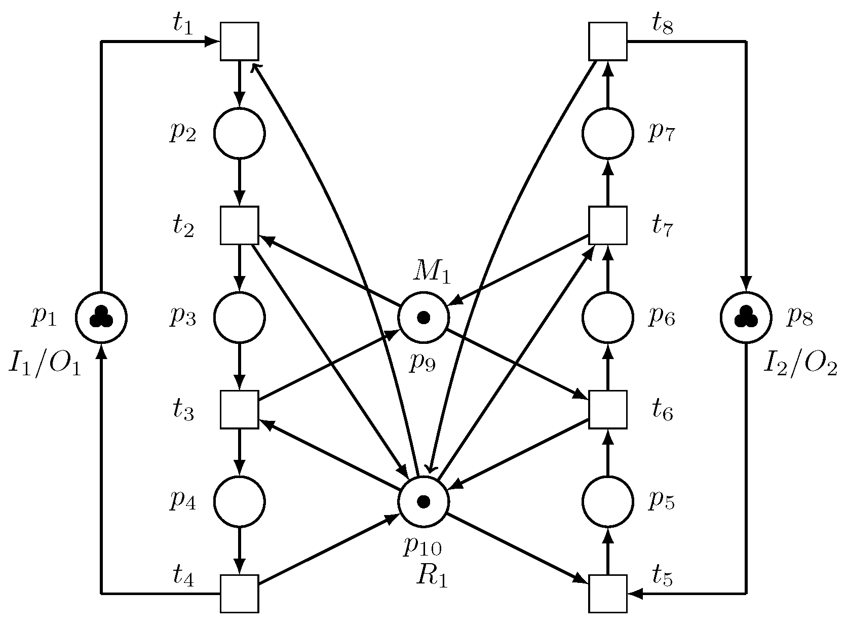
Example 1. 

Consider the robotic manufacturing cell in Figure 1, consisting of an unreliable robot $R_1$ performing the task of loading parts onto the machine $M_1$, which processes one part at a time. The parts are picked by the robot from two loading buffers $I_1$ and $I_2$. After the machine finishes processing a part, the robot unloads it onto the unloading buffers $O_1$ or $O_2$. The tasks that $R_1$ performs are represented by activities that are a holder of $R_1$, i.e., $H\left(p_{10}\right)=\{p_2,p_4,p_5,p_7\}$. The production sequences of the robotic cell are as follows:

$$\begin{array}{l}{J}_1:I_1\to R_1\to M_1\to R_1\to O_2\\ J_2:I_2\stackrel{}{\to }{R}_1\stackrel{}{\to }{M}_1\stackrel{}{\to }{R}_1\stackrel{}{\to }{O}_1\end{array}$$

The Petri net model of the robotic manufacturing cell is depicted in Figure 2. Since $R_1$ is an unreliable resource, designing only a deadlock controller for the system cannot guarantee a continued processing of parts by the manufacturing cell if $R_1$ fails. To increase the system’s reliability and improve the system performance, we propose the utilization of another robot that is reliable, or at least more reliable than $R_1$, which can perform the same task as $R_1$ to reduce the amount of tasks performed by $R_1$, and can perform all the tasks being performed by $R_1$ if $R_1$ fails.

3. Synthesis Method of AMS with LSRE

In this section, we first present the model of an AMS with an LSRE via an example such that a reader can readily capture the physical idea under the stated methodology.

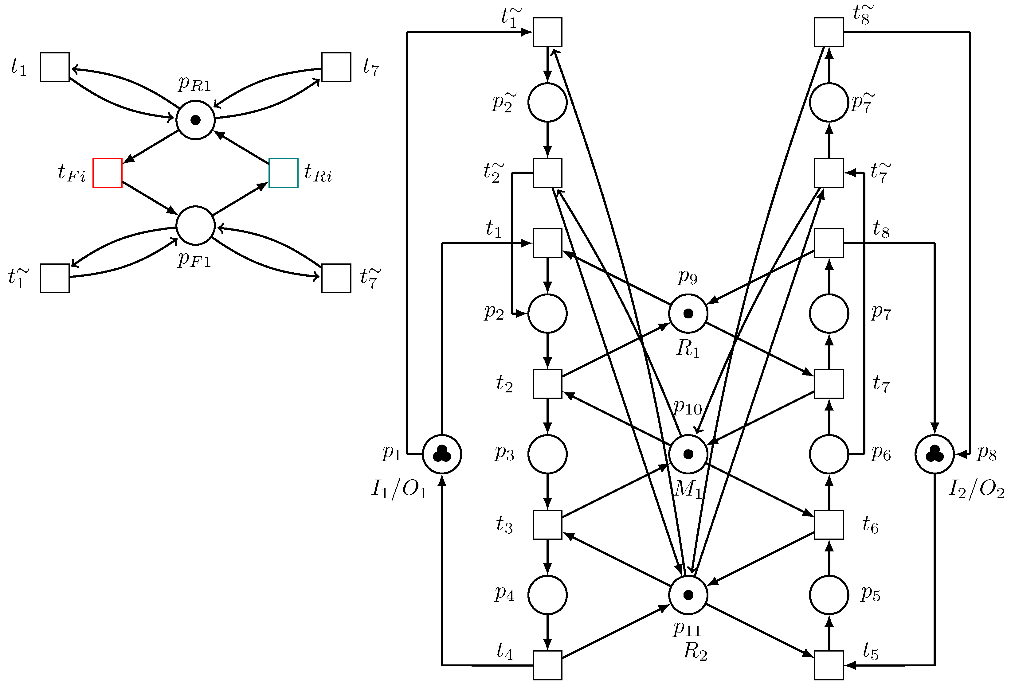
Example 2. 

Consider the system in Figure 1. It is a fact that when $R_1$ fails, all the processes in the system stop. If a robot $R_2$ that is reliable is introduced as an LSRE, both $R_1$ and $R_2$ can actively load and unload parts to/from $M_1$, and if $R_1$ fails, $R_2$ can step up and take over performing the tasks of loading and unloading the parts until $R_1$ is repaired. This fact is depicted in Figure 3 and the Petri net model of the manufacturing cell is visualized in Figure 4. The production sequence of the new robotic manufacturing cell becomes:

$$\begin{array}{c}{J}_1:I_1\to R_1\to M_1\to R_2\to O_2\\ J_2:I_2\stackrel{}{\to }{R}_2\stackrel{}{\to }{M}_1\stackrel{}{\to }{R}_1\stackrel{}{\to }{O}_1\end{array}$$

The tasks of loading or unloading parts are shared equally by $R_1$ and the added LSRE $R_2$. The tasks represented by activity places $p_4$ and $p_5$ that are being performed by $R_1$ in Example 1 are no longer performed by $R_1$. They are now being taken care of by $R_2$. Hence, $p_4$ and $p_5$ become holders of $R_2$, i.e., $H\left(p_{11}\right)=\{p_4,p_5\}$ and the set of holders of $R_1$ becomes $H\left(p_9\right)=\{p_2,p_7\}$. The following definition can naturally be derived from Example 2.

Definition 2. 

Let $(N_u,M_{u0})=(P_A\cup P^0\cup P_R,T,F,M_0)$ be a marked US${}^3$PR of an AMS with an unreliable target resource $r_u$. Let $H\left(r_u\right)={}^{••}{r}_u\cap P_A$ be the set of activity places that form the holder of $r_u$. A resource $r_s$ is said to be an LSRE of $r_u$ if (i) $\left|H\right(r_u\left)\right|>1$, (ii) it shares the tasks with $r_u$ such that there exists an activity place $p\in H\left(r_u\right)$ such that $p\in H\left(r_s\right)$ and $p\notin H\left(r_u\right)$ hold after the introduction of $r_s$ into the system, and (iii) it can perform all the tasks of $r_u$ in the event of an $r_u$ failure.

Remark 1. 

From Definition 2 and Example 2, the introduction of an LSRE $r_s$ is done by connecting $r_s$ to the input and output transitions of $p\in H\left(r_u\right)$ via arcs and removing all the arcs connecting $r_u$ to the input and output transitions of p.

Definition 3. 

Let $(N_u,M_{u0})=(P_A\cup P^0\cup P_R,T,F,M_0)$ be a marked U$S^3$PR of an AMS with an unreliable $r_u$ target. Let $(N_s,M_{s0})=(\left\{r_s\right\}$, $\{t\mid t\in {}^{•}p\cap p^{•}\}$, $F_{r_s},M_{s0})$ be the subnet of the load-sharing redundant element, where $r_s$ is the load-sharing redundant element, $p\in H\left(r_u\right)$ and $F_{r_s}=\{(r_s,t\in {}^{•}p),(t\in p^{•},r_s)\}$. An S${}^3$PR with an added load-sharing element is an S${}^3$PR Petri net model denoted by SU-S${}^3$PR and defined as $(N_{su},M_{su0})=(N_u,M_{u0})\parallel (N_s,M_{s0})$.

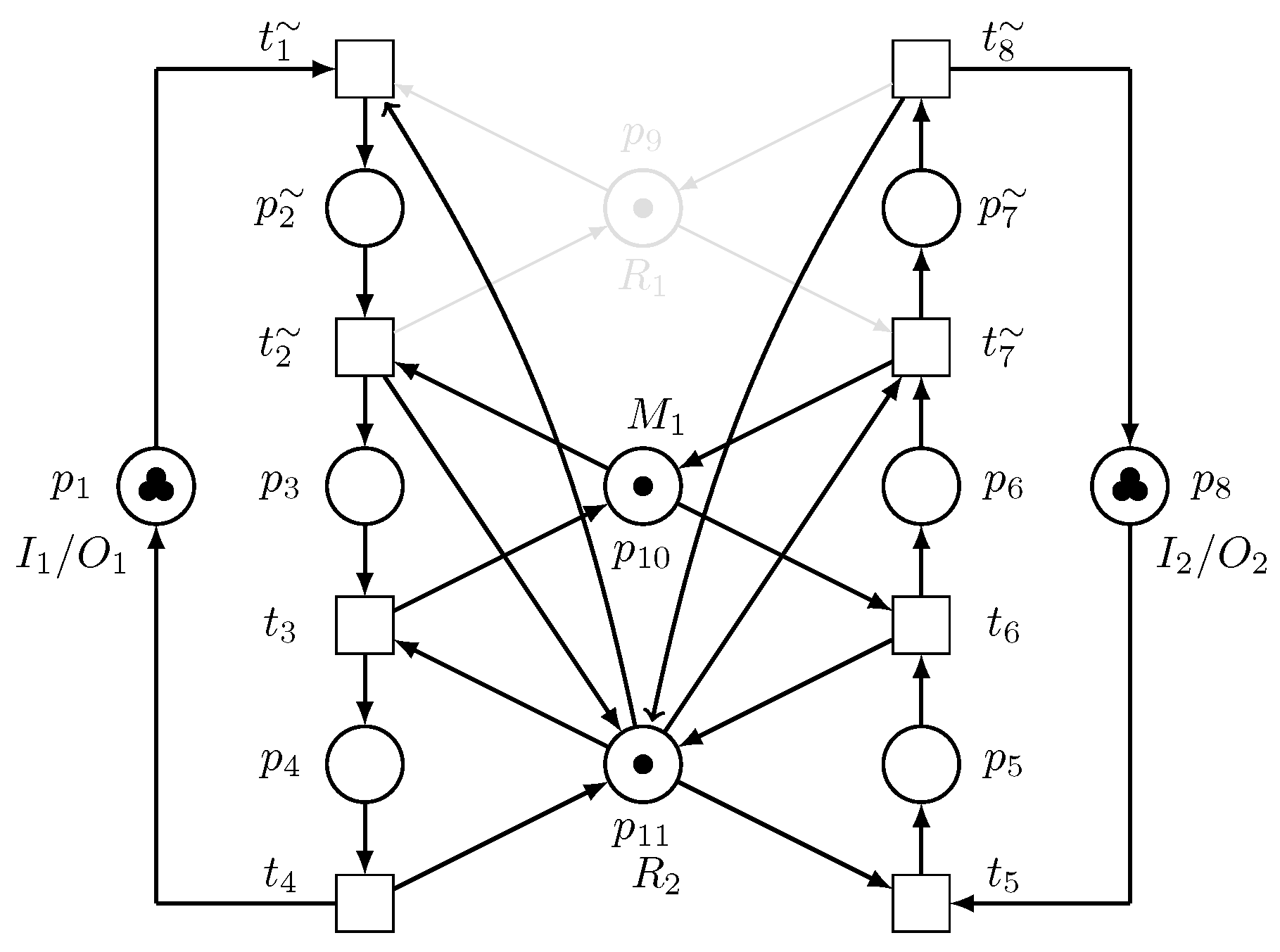
If the unreliable target resource $r_u$ fails, the load-sharing redundant element $r_s$ becomes the only resource that is operating and performing all the tasks. The Petri net model $(N_{su},M_{su0})$ obtained as a result of adding an LSRE $r_s$ to a Petri net of an AMS with unreliable resource $r_u$ does not model the failure and recovery of $r_u$ and how $r_s$ can process parts that are supposed to be processed by $r_u$ if $r_u$ fails. In this case, we need a switch subnet that models the failure and recovery of $r_u$. The switch submodel is a controller that is switched on when $r_u$ fails in order for $r_s$ to take over and process any $p\in H\left(r_u\right)$; when $r_u$ is repaired, the controller is switched off and $r_u$ resumes processing the parts that require it.

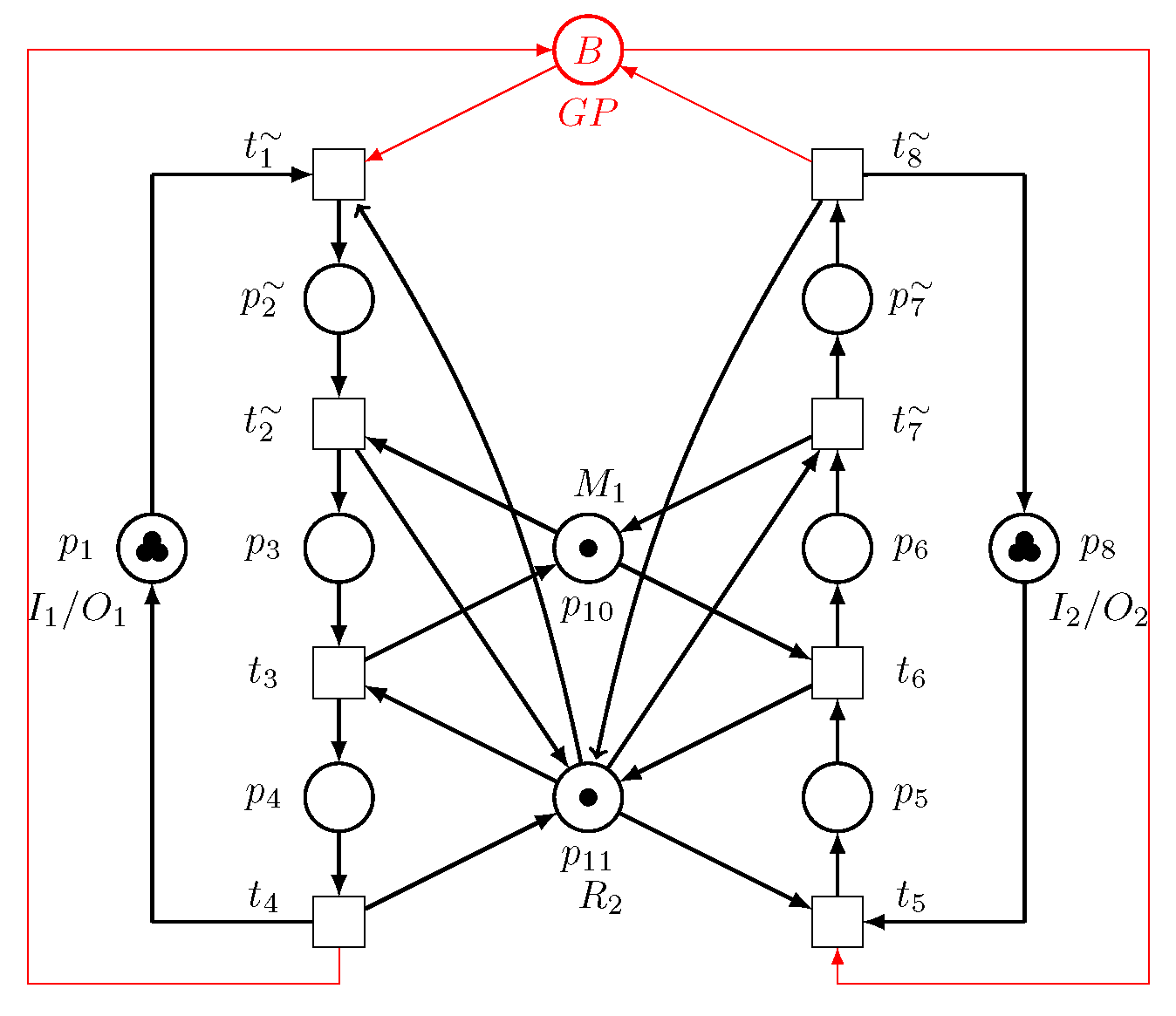
Definition 4. 

Let $(N_{su},M_{su0})$ be a Petri net of an AMS with an unreliable target element and an LSRE. Let $(N_{fru},M_{fru0})=(\{r_s,p_{Ru},p_{Fu},p_j^{\sim }\},\{t_{Fu},t_{Ru},t_{j-1}^{\sim }$, $t_j^{\sim }\}$, $F_{ru})$ be a switch submodel, where $r_s$ is the load-sharing redundant resource, $p_{Ru}$ represents the condition under which an unreliable resource $r_u$ is operational, $p_{Fu}$ models the failure of $r_u$, $p_j^{\sim }$ represents the condition in which $r_s$ is processing $p_j\in H\left(r_u\right)$ under the failure of $r_u$, $t_{Fu}$ denotes the failure event of $r_u$, $t_{Ru}$ is the recovery event of $r_u$, $t_{Ru}\in {{}^{•}p}_j^{\sim }$, and $t_j^{\sim }\in p_j^{\sim •}$. Moreover, we define

$$\begin{array}{c}{F}_{ru}=\{(p_{Ru},t_{j-1})(t_{j-1},p_{Ru}),(p_{Ru},t_{Fu}),(t_{Fu},p_{Fu}),(p_{Fu},t_{Ru}),(p_{Fu},t_{j-1}^{\sim }),\\ (t_{j-1}^{\sim },p_{Fu}),(r_u,t_{j-1}^{\sim }),(t_{j-1}^{\sim },p_j^{\sim }),(p_j^{\sim },t_j^{\sim }),(t_j^{\sim },r_u)\}\end{array}$$

Definition 5. 

Let $(N_{su},M_{su0})$ be a Petri net of an AMS with an unreliable target element and an added load-sharing redundant element, and let $(N_{fru},M_{fru0})$ be a switch submodel. A Petri net model with an unreliable element, an added load-sharing redundant element and a switch submodel is the composition of $(N_{su},M_{su0})$ and $(N_{fru},M_{fru0})$, denoted by $(N_F,M_{F0})=(N_{su},M_{su0})\otimes (N_{fru}$, $M_{fru0})$, where ⊗ defines the composition of two Petri net models.

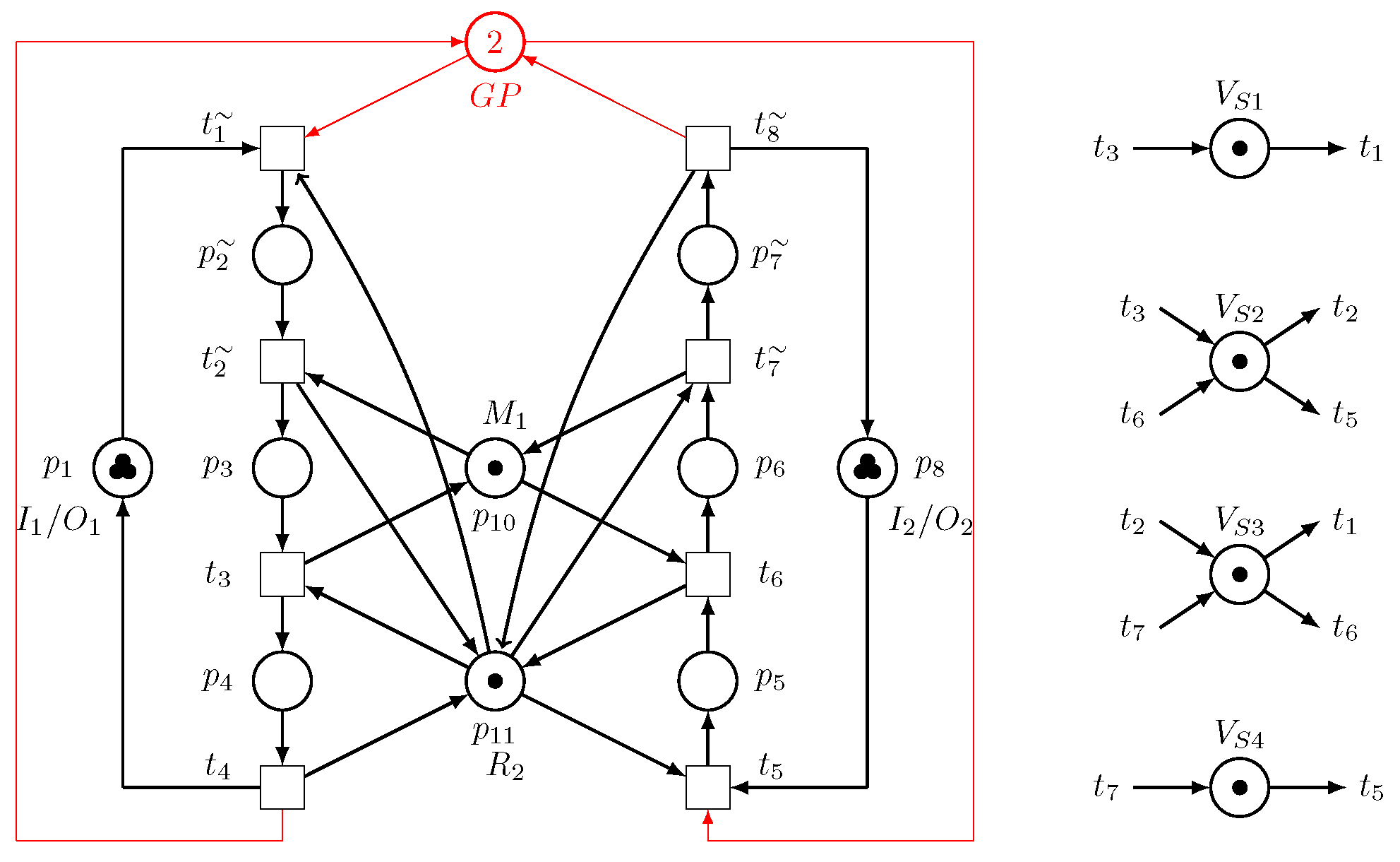
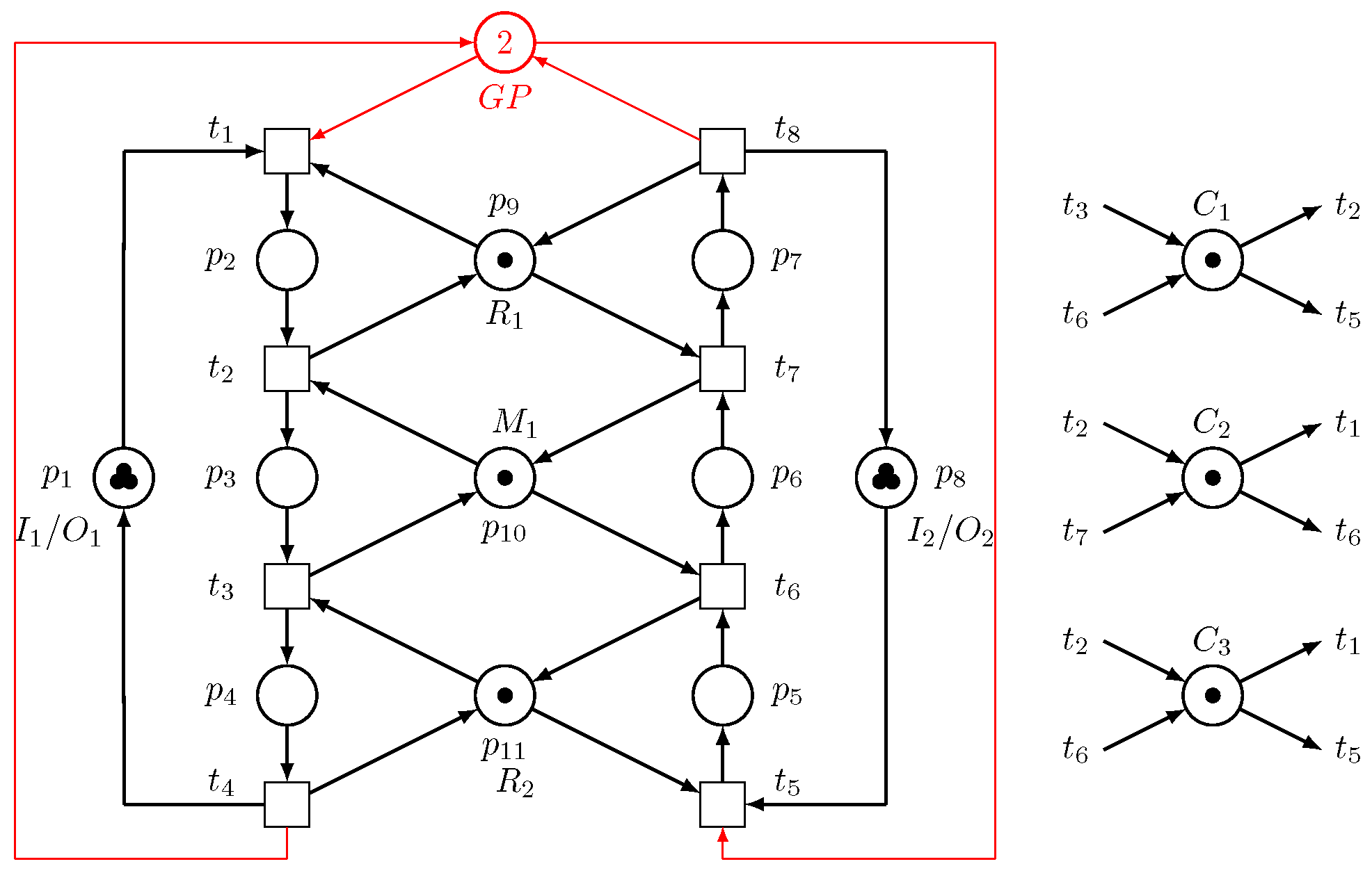
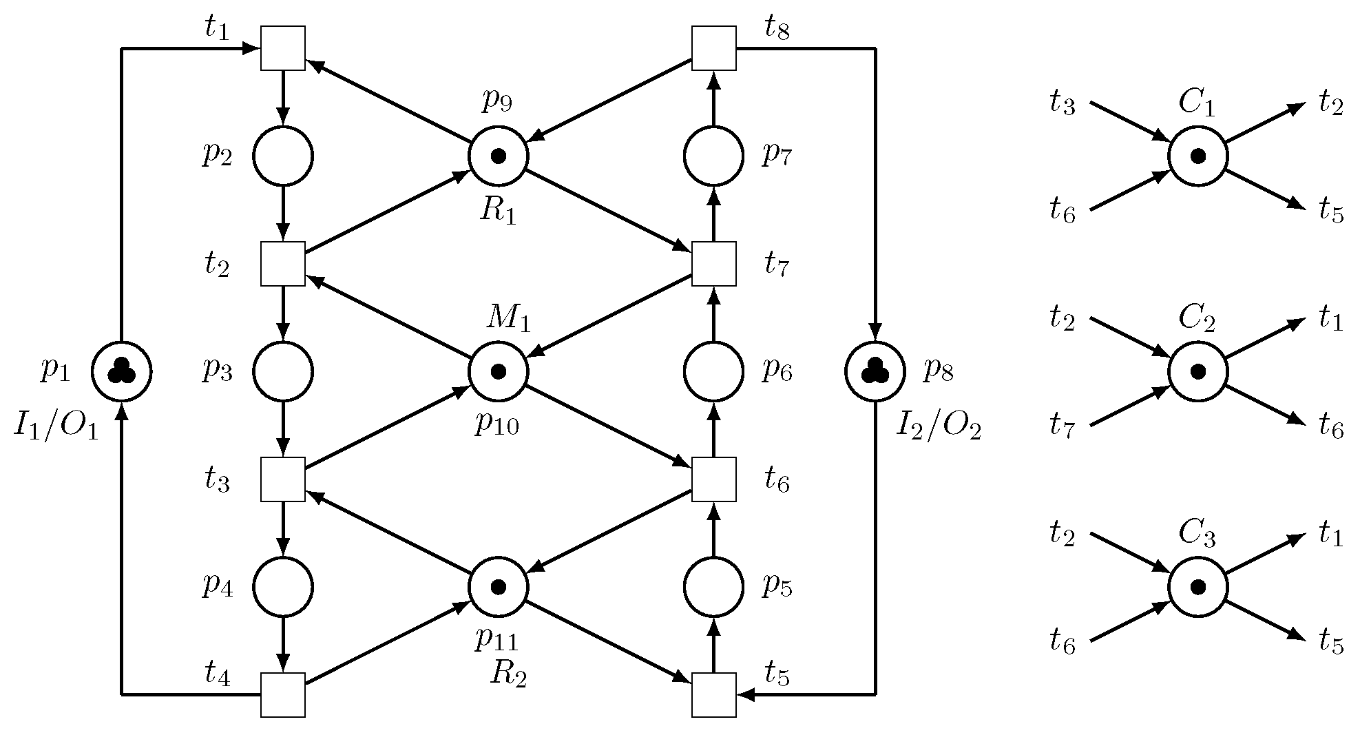
Example 3. 

Figure 5 shows the switch submodel of the unreliable target element $r_1$ of Figure 5 and Figure 6 represents the Petri net model of the system with an added switch submodel. Figure 7 shows what the system will be like with only the load-sharing redundant element operating, while Figure 8 describes what the Petri net model of the system will be like if both unreliable and loading sharing redundant resources (robots) are operating. The function of the switch submodel is to switch between these two conditions whenever there are failures and recoveries in the system.

4. Supervisory Controller Design for Automated Manufacturing Systems with LSRE

4.1. Controller Synthesis Based on Think Global, Act Locally Approach

This section proposes a control strategy for Petri nets modeling AMSs with a load-sharing redundant element, which comprises three stages. In the first stage, a supervisory controller is designed based on the deadlock control policy proposed in [50] for a Petri net model of the system under the failure of the target element, i.e., with only the redundant element carrying out all the tasks. In the second stage, a supervisory control is designed for the Petri net model of the system with an unreliable target element and a load-sharing redundant element. In the third stage, two Petri net models resulting from the first and second stages are composed and merged as a unified Petri net model, and deadlocks that may exist as a result of their combination are resolved. In the third stage, a switch submodel that models the failure of a target element and its recovery is designed and added to the resulting combined Petri net model. Moreover, redundant control places from the resulting final model are identified and removed such that the controlled system is structurally reduced.

In [50], an approach for computing liveness-enforcing supervisors (LESs) for AMSs was proposed, namely the think global, act locally approach (TGAL). A place named a global sink/source place (GP) was added to decide on a collection of monitors that could remove deadlock states. The TGAL technique is an iterative method with a complete state enumeration generated at each step without solving integer linear programming (ILP) problems. The resulting LES is often maximally permissive or suboptimal. In what follows, we recapitulate the concepts of TGAL as presented in [50].

The technique proposed in [50] generated an optimal LES. The condition was investigated using the well-established concepts of a minimal covered set of first-met bad markings (FBMs) and a minimal covering set of legal markings [51,52]. For the sake of readability and understandability, we recall the notions of FBMs, legal markings, minimal covered set of FBMs, and minimal covering set of legal markings.

Definition 6 

([52]). Given a Petri net system $(N,M_0)$, let M and $M^{\prime }$ be two markings in $R\left(N,M_0\right)$. Marking $M^{\prime }$ is said to be A-covered by M (or M A-covers $M^{\prime }$) if for all $p\in P_A$, $M\left(p\right)\ge M^{\prime }\left(p\right)$, which is denoted by $M^{\prime }{\le }_{\mathrm{A}}M$ (or $M{\ge }_{\mathrm{A}}{M}^{\prime }$ ).

The competition of resources in AMSs, as disclosed by Chen et al. [53], causes deadlocks in an AMS. A resource-processing unit is occupied when an activity place is marked with one token. As a result, deadlocks can only be deduced from token distribution in activity places.

Definition 7 

([52]). Let $M_{FBM}$ and $M_L$ denote the sets of markings in the deadlock zone ($DZ$) and live zone ($LZ$), respectively. $M_{FBM}^{*}$ and $M_L^{*}$ are said to be the minimal covered set of FBMs and the minimal covering set of legal markings, respectively, if the following statements are confirmed: (1) For all $M\in M_{FBM}$, there exists $M^{\prime }\in M_{\mathrm{FBM}}^{*}$ such that $M{\ge }_{\mathrm{A}}{M}^{\prime }$; (2) For all $M\in M_{\mathrm{FBM}}^{*}$, there does not exist $M^{″}\in M_{\mathrm{FBM}}^{*}$ such that $M^{″}{\ge }_{\mathrm{A}}M$ and $M^{″}=M$; (3) For all $M\in M_L$, there exists $M^{\prime }\in M_L^{*}$ such that $M^{\prime }{\ge }_{\mathrm{A}}M$; (4) For all $M\in M_L^{*}$, there does not exist $M^{″}\in M_L^{*}$ such that $M^{″}{\ge }_{\mathrm{A}}M$ and $M^{″}=M$.

Corollary 1 

([52]). All the markings in $M_L$ are reachable if all the markings in $M_L^{*}$ are reachable. All the markings in $M_{\mathrm{FBM}}$ are not reachable, if all the markings in $M_{\mathrm{FBM}}^{*}$ are forbidden by place invariants (PIs).

Let $P_A^M=\left\{p\mid p\in P_A,M\left(p\right)\ge 0\right\}$ and $M_B$ represent the set of bad markings in a PN model. It is said that bad markings are optimally controlled if their removal due to the constraints imposed by the additional PIs from the reachable space does not remove any marking in $M_L$. The condition is usually said to be the optimality condition under supervisory control in the DES community.

Corollary 2 

([50]). A bad marking (BM) M is optimally controlled if for all $M^{\prime }\in M_L^{*}$, ${\sum }_{p\in P_A}M\left(p\right)$$>{\sum }_{p\in P_A^M}{M}^{\prime }\left(p\right)$ holds.

Corollary 3 

([50]). If all the markings in $M_{\mathrm{FBM}}^{*}$ are optimally controlled, then all the BMs are optimally controlled.

Theorem 1 

([50]). If all bad markings are optimally controlled, Algorithm 1 generates an optimally controlled Petri net model (PNM) with optimal liveness.

The TGAL methodology presented in [22] improved the method reported in [50], where the method suggested obtained the local behavior of a given uncontrolled global PN model that is experiencing deadlocks by utilizing a global sink/source place (GP). The GP was associated with the global model in such a way that the number of tokens, denoted by B, placed into the GP, defined the total number of workpieces being processed within the model at a time. Parameter B was initially set to 1. That is, the model had only one workpiece in the first iteration. $N_1$ was the first local model. In this instance, if $N_1$ was not live, monitors were computed to enforce the liveness on the local model $N_1$. By increasing the number of computed monitors within $N_1$, the controlled model $N_1$ was acquired. The subsequent local model $N_2$ was determined by increasing the GP marking ($B=2$) of $N_1$. We repeated the preceding steps up until the final system was live. Since the monitors computed in earlier iterations were included in each local model, the DZ of the larger local models was kept smaller compared with the original uncontrolled local models. Algorithm 1 summarizes the technique of TGAL.

Algorithm 1: Think globally, act locally control method.

Input: A Petri net model (PNM)   Output: LES for the Petri net model 1 Step 1: Reduce the Petri net model (called reduced PNM–RPNM) as a result of PN reduction rules [54] (if the PNM does not have a huge RG, then the PNM can be utilized directly) 2 Step 2: Define all sink/source places $P_{S/S}$ of the RPNM’s input and output transitions 3 Add the GP to the RPNM (the input transitions of all sink/source places $P_{S/S}$ are the input transitions of the GP. Accordingly, the output transitions of all sink/source places $P_{S/S}$ are the GP output transitions. As a result, a new net system represented by $N_B$ = RPNM + GP is acquired, where $B\in N=\{1,2,\dots \}$). 4 Step 3:

Theorem 2 

([50]). The think globally, act locally strategy completes within finite steps if a considered Petri net model of an AMS is bounded.

Definition 8 

([55]). Let $\mathcal{N},{\mathcal{N}}^{\prime }\subseteq P_A$. Let $\tilde{\mathcal{N}}$ and ${\tilde{\mathcal{N}}}^{\prime }$ be constraints such that $\tilde{\mathcal{N}}=M\left(\mathcal{N}\right)<b$ and ${\tilde{\mathcal{N}}}^{\prime }=M\left({\mathcal{N}}^{\prime }\right)\le c$, with $b,c\in {\mathbb{N}}^{+}$. Constraint $\tilde{\mathcal{N}}$ is said to be redundant if $\tilde{\mathcal{N}}\subseteq {\tilde{\mathcal{N}}}^{\prime }$ and $c\le b$.

4.2. Illustrative Example

The corresponding Petri net model shown in Figure 7 with only $r_2$ operational has 8 transitions and 10 places with $P_A=$$\{p_2-p_7\},P^0=\{p_1,p_8\}$, and $P_R=\{p_{10},p_{11}\}$. There are 15 reachable states, 1 of which is a bad state, that is, a maximally permissive LES should have 14 states. We have $M_{\mathrm{FBM}}=\{p_2+p_5,p_3+p_5,p_2+p_6\}$ and $M_L=\left\{p_5+p_6+p_7\right.$, $\left.p_2+p_3+p_4\right\}$. Consequently, for all markings $M\in M_{FBM}^{*}$, for all $M^{\prime }\in M_L^{*}$, ${\sum }_{p\in P_A}M\left(p\right)>{\sum }_{p\in P_A^M}{M}^{\prime }\left(p\right)$ is true. We reach the conclusion that an ideal supervisor for this system can be found using the TGAL method.

• Step 1: Since the PN model does have a small reachability graph, the PN model is utilized directly without reducing its size.
• Step 2: For sink/source places $p_8$ and $p_1$, we have ${}^{•}{p}_8=\left\{t_8\right\}$, ${}^{•}{p}_1=\left\{t_4\right\}$, $p_8^{•}=\left\{t_5\right\}$, and $p_1^{•}=\left\{t_1\right\}$. We have ${}^{•}GP=\{t_4,t_8\}$ and $G{P}^{•}=\{t_1,t_5\}$. By including the GP, a novel net structure $N_B=PNM+GP$ is found, as illustrated in Figure 9.
• Step 3:

  (a)

  Step 3.1: ($B=1$) When one token is placed on the GP with seven good states, $N_1$ is live. $B:=B+1=2$.

  (b)

  Step 3.2:

  i.

  ($B=2$) $N_2$ is found when the GP is designated by two tokens, as illustrated in Figure 10. $N_2$ is not live with 11 states within the $R{G}_2$ of $N_2$. $D{Z}_2$ has four bad states; $B{M}_1$ and $L{Z}_2$ contain seven good states.

  ii.

  Table 1. Markings of activity places $B{M}_1$, $B{M}_2$, $B{M}_3$, and $B{M}_4$.

  State Number	${\mathit{p}}_2$	${\mathit{p}}_3$	${\mathit{p}}_4$	${\mathit{p}}_5$	${\mathit{p}}_6$	${\mathit{p}}_7$
  $S_4$	1	1	0	0	0	0
  $S_6$	0	1	0	1	0	0
  $S_9$	1	0	0	0	1	0
  $S_{10}$	1	1	0	1	1	0

  depicts the indications of the activity places of $B{M}_1$, $B{M}_2$, $B{M}_3$, and $B{M}_4$.

  The following place invariants are created in order not to approach $B{M}_1$, $B{M}_2$, $B{M}_3$, and $B{M}_4$, respectively:

  $$\begin{array}{c}P{I}_1={\mu }_2+{\mu }_3\le 1,\\ P{I}_2={\mu }_3+{\mu }_5\le 1,\\ P{I}_3={\mu }_2+{\mu }_6\le 1,\\ P{I}_4={\mu }_5+{\mu }_6\le 1.\end{array}$$

  iii.

  Monitors $V_{S1}$, $V_{S2}$, $V_{S3}$, and $V_{S4}$ are computed in order to enforce $P{I}_1$, $P{I}_2$, $P{I}_3$, and $P{I}_4$, respectively, as shown in

  Table 2. Computed monitors $V_{S1},V_{S2},V_{S3}$, and $V_{S4}$ for $P{I}_1$, $P{I}_2$, $P{I}_3$, and $P{I}_4$, respectively.

  ${\mathit{C}}_{\mathit{i}}$	${}^{•}{\mathit{V}}_{\mathit{Si}}$	${\mathit{V}}_{\mathit{Si}}^{•}$	${\mathit{\mu }}_0\left({\mathit{V}}_{\mathit{Si}}\right)$
  $V_{S1}$	$t_3$	$t_1^{\sim }$	1
  $V_{S2}$	$t_3$, $t_6$	$t_2^{\sim }$, $t_5$	1
  $V_{S3}$	$t_2^{\sim }$, $t_7^{\sim }$	$t_1^{\sim }$, $t_6$	1
  $V_{S4}$	$t_7^{\sim }$	$t_5$	1

  .

  iv.

  Since only one monitor is derived, no redundancy test is performed.

  v.

  When the uncontrolled model $N_2$ is augmented with $V_{S1}$, $V_{S2}$, $V_{S3}$, and $V_{S4}$, the controlled $N_2$ is acquired as follows: $N_2$:= $N_2+V_{S1}+V_{S2}+V_{S3}+V_{S4}$, as shown in Figure 10. $N_2$, illustrated in Figure 11, is live with seven good states, i.e., it is ideal. $B:=B+1=3$.

  (c)

  Step 3.3: ($B=3$) The net $N_3$, as illustrated in Figure 12, is acquired by increasing the number of tokens in the GP while keeping the controlled $N_2$ constant. With seven good states, $N_3$ is live, which is the optimal solution to both the original uncontrolled PN model and $N_3$.

The Petri net model shown in Figure 4 has 8 transitions and 11 places with $P_A=$$\left\{p_2-p_7\right\},P^0=\left\{p_1,p_8\right\}$, and $P_R=\left\{p_9-p_{11}\right\}$. There are 5 bad states out of the 20 reachable states; thus, a maximally permissive LES should contain 15 states. We have $M_{FBM}=\left\{p_2+p_6,p_3+p_5,p_2+p_5\right\}$ and $M_L=\left\{p_5+p_6+p_7\right.$, $\left.p_2+p_3+p_4\right\}$. Thus, for all markings $M\in M_{FBM}^{*}$, for all $M^{\prime }\in M_L^{*}$, ${\sum }_{p\in P_A}M\left(p\right)>{\sum }_{p\in P_A^M}{M}^{\prime }\left(p\right)$ is true. We reach the conclusion that an ideal supervisor for this system can be found using the TGAL method.

• Step 1: Since the PNM does have a small RG, the PNM is utilized directly without reducing the PNM.
• Step 2: For sink/source places $p_8$ and $p_1$, we have ${}^{•}{p}_8=\left\{t_8\right\}$, ${}^{•}{p}_1=\left\{t_4\right\}$, $p_8^{•}=\left\{t_5\right\}$, and $p_1^{•}=\left\{t_1\right\}$. Thus, ${}^{•}GP=\{t_4,t_8\}$ and $G{P}^{•}=\{t_1,t_5\}$. By including the GP, a novel net structure $N_B=PNM+GP$ is found, as illustrated in Figure 13.
• Step 3:

  (a)

  Step 3.1: ($B=1$). When one token is placed on the GP with seven good states, $N_1$ is live. $B:=B+1=2$.

  (b)

  Step 3.2:

  i.

  ($B=2$) $N_2$ is found when two tokens are marked to the GP, as illustrated in Figure 14. With 17 states in the $R{G}_2$ of $N_2$, $N_2$ is not live. $B{M}_1$ and $L{Z}_2$ have 14 good states, whereas $D{Z}_2$ has 3 bad states.

  ii.

  Table 3. Markings of activity places $B{M}_1$, $B{M}_2$, and $B{M}_3$.

  State Number	${\mathit{p}}_2$	${\mathit{p}}_3$	${\mathit{p}}_4$	${\mathit{p}}_5$	${\mathit{p}}_6$	${\mathit{p}}_7$
  $S_8$	0	1	0	1	0	0
  $S_{10}$	1	0	0	0	1	0
  $S_{11}$	1	0	0	1	0	0

  displays the markings of the activity places $B{M}_1$, $B{M}_2$, and $B{M}_3$. The following place invariants are established, accordingly, in order not to overreach $B{M}_1$, $B{M}_2$, and $B{M}_3$, respectively:

  $$\begin{array}{c}P{I}_1={\mu }_3+{\mu }_5\le 1,\\ P{I}_2={\mu }_2+{\mu }_6\le 1,\\ P{I}_3={\mu }_2+{\mu }_5\le 1.\end{array}$$

  iii.

  Monitors $C_1$, $C_2$, and $C_3$ are computed in order to enforce $P{I}_1$, $P{I}_2$, and $P{I}_3$, respectively, as shown in

  Table 4. $C_1$, $C_2$, and $C_3$ are the computed monitors for $P{I}_1$, $P{I}_2$, and $P{I}_3$.

  ${\mathit{C}}_{\mathit{i}}$	${}^{•}{\mathit{C}}_{\mathit{i}}$	${\mathit{C}}_{\mathit{i}}^{•}$	${\mathit{\mu }}_0\left({\mathit{C}}_{\mathit{i}}\right)$
  $C_1$	$t_3$, $t_6$	$t_2$, $t_5$	1
  $C_2$	$t_2$, $t_7$	$t_1$, $t_6$	1
  $C_3$	$t_2$, $t_6$	$t_1$, $t_5$	1

  .

  iv.

  Since only one monitor is derived, no redundancy test is performed.

  v.

  When the uncontrolled model $N_2$ is augmented utilizing $C_1$, $C_2$, and $C_3$, the controlled $N_2$ is produced as follows: $N_2$:= $N_2+C_1+C_2+C_3$, as displayed in Figure 14.

  $N_2$, as illustrated in Figure 15, is live with 14 good states, i.e., it is ideal. $B:=B+1=3$.

  (c)

  Step 3.3: The net $N_3$ ($B=3$), as displayed in Figure 16, is acquired by increasing the number of tokens in the GP while keeping the controlled $N_2$ constant. With 14 good states, $N_3$ is live, which is the optimal resolution for both the original uncontrolled PNM and $N_3$.

In this stage, two Petri net models resulting from the first and the second stages are merged as a unified Petri net model and deadlocks that may exist as a result of their combination are resolved as shown in Figure 17. In addition, redundant control places from the resulting final model are identified and removed. For example, we find that the control places $V_{S2}$ and $C_1$ in both Figure 12 and Figure 16, respectively, both have one token, ${}^{•}{V}_{S2}$ = ${}^{•}{C}_1$=$\{t_3,t_6\}$, and $V_{S2}^{•}$ = $C_1^{•}$=$\{t_2,t_5\}$. Moreover, $V_{S3}$ and $C_2$ in Figure 12 and Figure 16 both have one token ${}^{•}{V}_{S3}$ = ${}^{•}{C}_2$=$\{t_2,t_7\}$, and $V_{S3}^{•}$ = $C_2^{•}$=$\{t_1,t_6\}$.

5. Experimental Results

This section uses real-world examples with a significant state space to demonstrate the applicability and efficacy of our suggested strategy.

Example 4. 

Consider a robotic manufacturing cell [56] consisting of two loading buffers $I_1$–$I_2$, four machines $M_1$–$M_4$, two robots $r_1$–$r_2$ ($r_1$ introduced as an LSRE and $r_2$ an unreliable robot), and two unloading buffers $O_1$–$O_2$, as shown in Figure 18. Its Petri net model of the AMS is shown in Figure 19. There are 14 transitions and 19 places. It has the following place partitions: $P_A=\{p_2,\dots ,p_7,p_9,\dots ,p_{13}\}$, $P_R=\{p_{14},\dots ,p_{19}\}$, and $P^0=\{p_1,p_8\}$. It has 282 reachable states, 77 of which are bad states and thus, a maximally permissive LES should have 205 states.

Consider the system operating using the load-sharing redundant robot $r_1$ only, i.e., an unreliable robot $r_2$ fails, as shown in Figure 20. In this case, the monitors are provided for a Petri net model using the TGAL method, as shown in

Table 5. Monitors computed for the Petri net model of the AMS [56] shown in Figure 20.

${\mathit{BM}}_{\mathit{i}}$	${\mathit{PI}}_{\mathit{i}}$	${\mathit{V}}_{\mathit{Si}}$	${}^{•}{\mathit{V}}_{\mathit{Si}}$	${\mathit{V}}_{\mathit{Si}}^{•}$	${\mathit{\mu }}_0\left({\mathit{V}}_{\mathit{Si}}\right)$
${\mu }_5=1,{\mu }_6=1$	${\mu }_5+{\mu }_6\le 1$	$V_{S1}$	$t_7^{\sim }$	$t_4$, $t_5$	1
${\mu }_3=1,{\mu }_{11}=1$	${\mu }_3+{\mu }_{11}\le 1$	$V_{S2}$	$t_5$, $t_{12}$	$t_2$,$t_{11}$	1
${\mu }_{11}=1,{\mu }_{12}=1$	${\mu }_{11}+{\mu }_{12}\le 1$	$V_{S3}$	$t_{13}$	$t_{11}$	1
${\mu }_9=1,{\mu }_{10}=1$	${\mu }_9+{\mu }_{10}\le 1$	$V_{S4}$	$t_{11}$	$t_9^{\sim }$	1
${\mu }_2=1,{\mu }_3=1,{\mu }_4=1$	${\mu }_2+{\mu }_3+{\mu }_4\le 2$	$V_{S5}$	$t_4$,$t_5$	$t_1$	2
${\mu }_2=1,{\mu }_4=1,{\mu }_{12}=1$	${\mu }_2+{\mu }_4+{\mu }_{12}\le 2$	$V_{S6}$	$t_2$, $t_4$,$t_{13}$	$t_1$, $t_{12}$	2

.

In the case when both unreliable and loading-sharing redundant resources (robots) are operating, i.e., an unreliable robot $r_2$ is not a failure, as depicted in Figure 21, the monitors for the Petri net model are provided using the TGAL method, as shown in

Table 6. Monitors computed for the Petri net model of the AMS [56] shown in Figure 21.

${\mathit{BM}}_{\mathit{i}}$	${\mathit{PI}}_{\mathit{i}}$	${\mathit{C}}_{\mathit{i}}$	${}^{•}{\mathit{C}}_{\mathit{i}}$	${\mathit{C}}_{\mathit{i}}^{•}$	${\mathit{\mu }}_0\left({\mathit{C}}_{\mathit{i}}\right)$
${\mu }_3=1,{\mu }_{11}=1$	${\mu }_3+{\mu }_{11}\le 1$	$C_1$	$t_2$, $t_5$	$t_1$, $t_{11}$	1
${\mu }_{11}=1,{\mu }_{12}=1$	${\mu }_{11}+{\mu }_{12}\le 1$	$C_2$	$t_{13}$	$t_{11}$	1
${\mu }_2=1,{\mu }_3=1,{\mu }_4=1$	${\mu }_2+{\mu }_3+{\mu }_4\le 2$	$C_3$	$t_5$, $t_4$	$t_1$	2
${\mu }_2=1,{\mu }_4=1,{\mu }_{12}=1$	${\mu }_2+{\mu }_4+{\mu }_{12}$		$t_{13}$, $t_4$,	$t_{12}$,$t_1$
	$\le 2$	$C_4$	$t_2$		2
${\mu }_5=1,{\mu }_6=1,{\mu }_9=1,$	${\mu }_5+{\mu }_6+{\mu }_9+$		$t_{11}$,$t_7$	$t_9$, $t_5$,
${\mu }_{10}=1$	${\mu }_{10}\le 2$	$C_5$		$t_4$	3
${\mu }_3=1,{\mu }_6=1,{\mu }_9=1,$	${\mu }_3+{\mu }_6+{\mu }_9+$		$t_{11}$, $t_7$,	$t_9$, $t_6$,
${\mu }_{10}=1$	${\mu }_{10}\le 3$	$C_6$	$t_5$	$t_2$	3
${\mu }_3=1,{\mu }_5=1,{\mu }_9=1,$	${\mu }_3+{\mu }_5+{\mu }_9+$		$t_{11}$, $t_6$	$t_9$, $t_4$,
${\mu }_{10}=1$	${\mu }_{10}\le 3$	$C_7$		$t_2$	3
${\mu }_2=1,{\mu }_4=1,{\mu }_6=1,$	${\mu }_2+{\mu }_4+{\mu }_6+$		$t_{11}$, $t_7$,	$t_9$, $t_6$,
${\mu }_9=1,{\mu }_{10}=1$	${\mu }_9+{\mu }_{10}\le 4$	$C_8$	$t_4$, $t_2$	$t_1$	4

.

In the third stage, the two Petri net models resulting from the first and second stages, respectively, are merged into a unified Petri net model, and any deadlocks that may have occurred as a result of their combination are addressed, as shown in Figure 22. Furthermore, redundant control places in the final model are discovered and deleted.

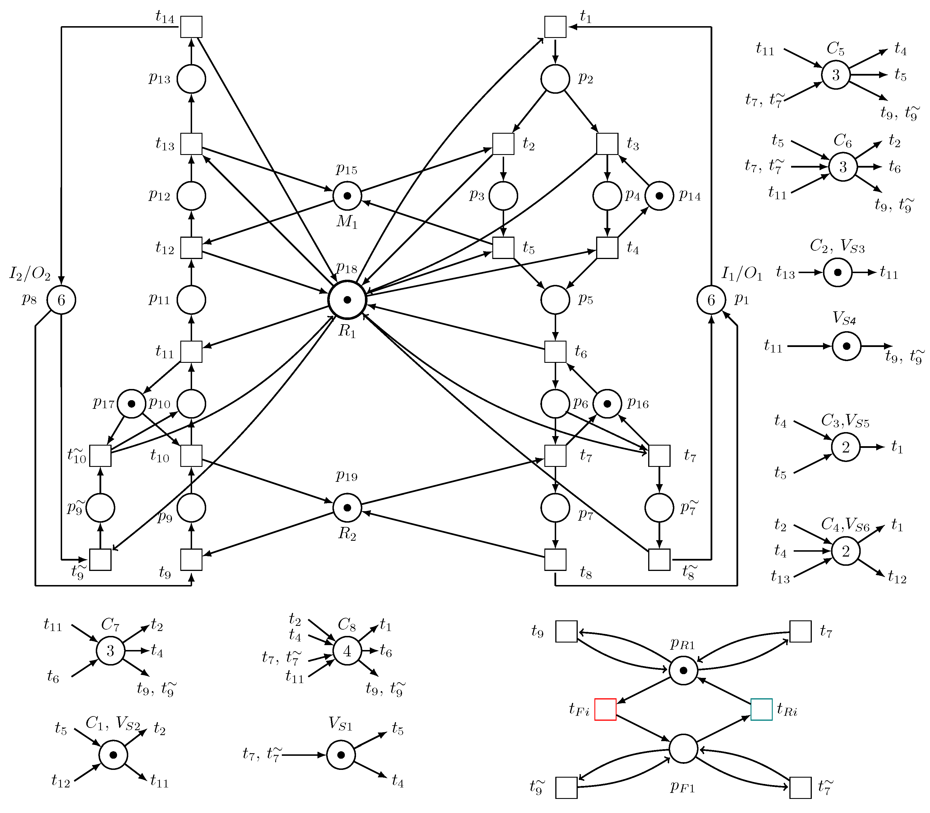
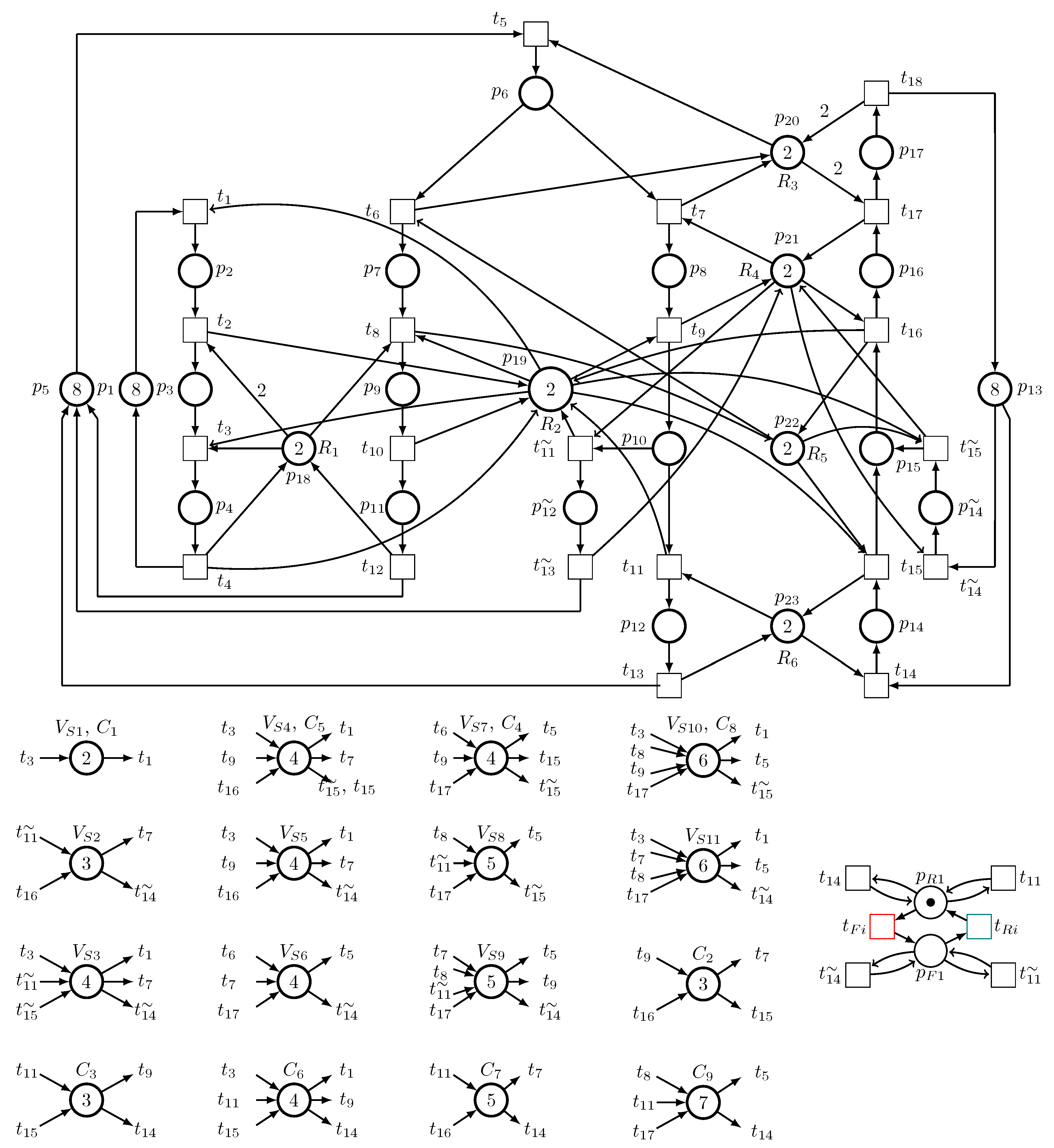
Example 5. 

Consider a robotic manufacturing cell [57] containing six robots, $r_1$–$r_6$ ($r_4$ introduced as an LSRE and $r_6$ an unreliable robot), and the S${}^4$R Petri net model of the manufacturing cell is visualized in Figure 23, where $T=\left\{t_1-t_{18}\right\}$, $P=\left\{p_1-p_{23}\right\}$, $P_R=\left\{p_{18}-p_{23}\right\}$, $P_{S/S}=\left\{p_1,p_5,p_{13}\right\},P_{A3}=\left\{p_{14}-p_{17}\right\}$, $P_{A2}=\left\{p_6-p_{12}\right\}$, and $P_{A1}=\left\{p_2-p_4\right\}$.

Consider the system operating using the load-sharing redundant robot $r_4$, i.e., an unreliable robot $r_6$ fails, as shown in Figure 24. In this case, the monitors are provided for a Petri net model using the TGAL method, as given in

Table 7. Monitors computed for the S${}^4$R Petri net model of the AMS [57] shown in Figure 24.

${\mathit{BM}}_{\mathit{i}}$	${\mathit{PI}}_{\mathit{i}}$	${\mathit{V}}_{\mathit{Si}}$	${}^{•}{\mathit{V}}_{\mathit{Si}}$	${\mathit{V}}_{\mathit{Si}}^{•}$	${\mathit{\mu }}_0\left({\mathit{V}}_{\mathit{Si}}\right)$
${\mu }_3=1,{\mu }_2=2$	${\mu }_3+2{\mu }_2\le 2$	$V_{S1}$	$t_3$	$t_1$	2
${\mu }_{15}=1,{\mu }_{14}=1,{\mu }_{10}=1,$	${\mu }_{15}+{\mu }_{14}+{\mu }_{10}+$		$t_{11}^{\sim }$, $t_{16}$	$t_7$,$t_{14}^{\sim }$
${\mu }_8=1$	${\mu }_8\le 3$	$V_{S2}$			3
${\mu }_{14}=1,{\mu }_{10}=1,{\mu }_8=1,$	${\mu }_{14}+{\mu }_{10}+{\mu }_8+$		$t_3$, $t_{11}^{\sim }$,	$t_1$, $t_7$,
${\mu }_3=1$, ${\mu }_2=1$	${\mu }_3+{\mu }_2\le 4$	$V_{S3}$	$t_{15}^{\sim }$	$t_{14}^{\sim }$	4
${\mu }_{15}=1,{\mu }_8=2$, ${\mu }_3=1,$	${\mu }_{15}+2{\mu }_8+{\mu }_3+$		$t_3$, $t_9$,	$t_1$, $t_7$,
${\mu }_2=1$	${\mu }_2\le 4$	$V_{S4}$	$t_{16}$	$t_{15}^{\sim }$	4
${\mu }_{15}=1,{\mu }_{14}=1$, ${\mu }_8=1,$	${\mu }_{15}+{\mu }_{14}+{\mu }_8+$		$t_3$, $t_9$,	$t_1$, $t_7$,
${\mu }_3=1$, ${\mu }_2=1$	${\mu }_3+{\mu }_2\le 4$	$V_{S5}$	$t_{16}$	$t_{14}^{\sim }$	4
${\mu }_{16}=1,{\mu }_{15}=2$, ${\mu }_{14}=1,$	${\mu }_{16}+2{\mu }_{15}+{\mu }_{14}+$		$t_6$, $t_7$,	$t_5$, $t_{14}^{\sim }$
${\mu }_6=1$	$+{\mu }_6\le 4$	$V_{S6}$	$t_{17}$		4
${\mu }_{16}=1,{\mu }_{15}=2$, ${\mu }_8=1,$	${\mu }_{16}+2{\mu }_{15}+{\mu }_8$		$t_6$, $t_9$,	$t_5$, $t_{15}^{\sim }$
${\mu }_6=1$	$+{\mu }_6\le 4$	$V_{S7}$	$t_{17}$		4
${\mu }_{16}=1,{\mu }_{15}=1,{\mu }_{10}=1$ ,	${\mu }_{16}+{\mu }_{15}+{\mu }_{10}+$		$t_8$, $t_{11}^{\sim }$,	$t_5$, $t_{15}^{\sim }$
${\mu }_8=1$, ${\mu }_7=1$, ${\mu }_6=1$	${\mu }_8+{\mu }_7+{\mu }_6\le 5$	$V_{S8}$	$t_{17}$		5
${\mu }_{16}=1,{\mu }_{15}=1,{\mu }_{14}=1$ ,	${\mu }_{16}+{\mu }_{15}+{\mu }_{14}+$		$t_7$, $t_8$,	$t_5$, $t_9$,
${\mu }_{10}=1,{\mu }_7=1,{\mu }_6=1$	${\mu }_{10}+{\mu }_7+{\mu }_6\le 5$	$V_{S9}$	$t_{11}^{\sim }$, $t_{17}$	$t_{14}^{\sim }$	5
${\mu }_{16}=1,{\mu }_{15}=1,{\mu }_8=1$ ,${\mu }_7=1,$	${\mu }_{16}+{\mu }_{15}+{\mu }_8+$		$t_3$, $t_8$,	$t_1$, $t_5$,
${\mu }_6=1,{\mu }_3=1,{\mu }_2=1$	${\mu }_7+{\mu }_6+{\mu }_3+{\mu }_2\le 6$	$V_{S10}$	$t_9$, $t_{17}$	$t_{15}$	6
${\mu }_{16}=1,{\mu }_{15}=1,{\mu }_{14}=1$,	${\mu }_{16}+{\mu }_{15}+{\mu }_{14}+$		$t_3$, $t_7$,	$t_1$, $t_5$,
${\mu }_7=1$, ${\mu }_6=1$, ${\mu }_3=1$, ${\mu }_2=1$	${\mu }_7+{\mu }_6+{\mu }_3+{\mu }_2\le 6$	$V_{S11}$	$t_8$, $t_{17}$	$t_{14}$	6

.

In the case when both unreliable and loading-sharing redundant resources (robots) are operating, i.e., an unreliable robot $r_4$ is not a failure, as depicted in Figure 25, the monitors for the Petri net model are provided using the TGAL method, as shown in

Table 8. Monitors computed for the S${}^4$R Petri net model of the AMS [57] shown in Figure 25.

$\mathit{B}{\mathit{M}}_{\mathit{i}}$	$\mathit{P}{\mathit{I}}_{\mathit{i}}$	${\mathit{C}}_{\mathit{i}}$	${}^{•}{\mathit{C}}_{\mathit{i}}$	${\mathit{C}}_{\mathit{i}}^{•}$	${\mathit{\mu }}_0\left({\mathit{C}}_{\mathit{i}}\right)$
${\mu }_2=2,{\mu }_3=1$	$2{\mu }_2+{\mu }_3\le 2$	$C_1$	$t_3$	$t_1$	2
${\mu }_8=2,{\mu }_{15}=2$	$2{\mu }_8+2{\mu }_{15}\le 3$	$C_2$	$t_{16}$, $t_9$	$t_{15}$, $t_7$	3
${\mu }_{10}=2,{\mu }_{14}=2$	$2{\mu }_{10}+2{\mu }_{14}\le 3$	$C_3$	$t_{15}$, $t_{11}$	$t_{14}$, $t_9$	3
${\mu }_6=1,{\mu }_8=1,{\mu }_{15}=2,$	${\mu }_6+{\mu }_8+2{\mu }_{15}+$		$t_{17}$, $t_9$,	$t_{15}$, $t_5$
${\mu }_{16}=1$	${\mu }_{16}\le 4$	$C_4$	$t_6$		4
${\mu }_2=1,{\mu }_3=1,{\mu }_8=2,$	${\mu }_2+{\mu }_3+2{\mu }_8+$		$t_{16}$, $t_9$,	$t_{15}$, $t_7$,
${\mu }_{15}=1$	${\mu }_{15}\le 4$	$C_5$	$t_3$	$t_1$	4
${\mu }_2=1,{\mu }_3=1,{\mu }_{10}=1,$	${\mu }_2+{\mu }_3+{\mu }_{10}+$		$t_{15}$,$t_{11}$,	$t_{14}$, $t_9$,
${\mu }_{14}=2$	${\mu }_{14}\le 4$	$C_6$	$t_3$	$t_1$	4
${\mu }_8=2,{\mu }_{10}=1,{\mu }_{14}=2,$	$2{\mu }_8+{\mu }_{10}+2{\mu }_{14}+$		$t_{16}$, $t_{11}$	$t_{14}$, $t_7$
${\mu }_{15}=1$	${\mu }_{15}\le 5$	$C_7$			5
${\mu }_{16}=1,{\mu }_{15}=1,{\mu }_8=1$,	${\mu }_2+{\mu }_3+{\mu }_6+{\mu }_7+$		$t_{17}$, $t_9$,	$t_{15}$, $t_5$,$t_1$
${\mu }_7=1,{\mu }_6=1,{\mu }_3=1,{\mu }_2=1$	${\mu }_8+{\mu }_{15}+{\mu }_{16}\le 6$	$C_8$	$t_3$, $t_8$		6
${\mu }_{16}=1,{\mu }_{15}=1,{\mu }_{14}=2$,	${\mu }_6+{\mu }_7+{\mu }_8+{\mu }_{10}+$		$t_{17}$, $t_{11}$,	$t_{14}$, $t_5$
${\mu }_{10}=1,{\mu }_8=1,{\mu }_7=1,{\mu }_6=1$	$2{\mu }_{14}+{\mu }_{15}+{\mu }_{16}\le 6$	$C_9$	$t_8$		7

.

The third stage is the merging stage, and in the following, two Petri net models resulting from the first stage and the second stage are merged as a unified Petri net model, and deadlocks that may exist as a result of their combination are resolved as shown in Figure 26. Moreover, redundant control places from the resulting final model are identified and removed.

Finally, simulation is an important method for evaluating the performance and validating a proposed method. TINA (TIme Petri Net Analyzer) is a software application that simulates, evaluates, and models discrete event systems using Petri net models [58]. To validate the proposed method, a simulation was performed using an applied example (the previous Example 1) based on TINA.

The proposed method was compared with the methods by Wu et al. [59] and Zhang et al. [60] for its testing and validation. In the simulation, we considered failures that happened to the target elements after a period of operation for the system over different time periods. We obtained the results as summarized in

Table 9. Comparison of time performance with the existing methods.

Performance	Wu et al. [59]	Zhang et al. [60]	The Proposed Method
Robot 1 utilization %	20.5	23.67	13.56
Machine utilization %	51.25	62.5	64.17
Robot 2 utilization %	20.33	25	37.5
Throughput time (parts/min)	45.86	35.77	32.08
Throughput (parts)	122	149	154

after running and simulating the Petri net model using TINA tools, which illustrated a comparison of the performance of the proposed method and that of other methods in the literature. Figure 27 depicts the results in terms of machine and robot utilization, the throughput of parts $J_1$ and $J_2$, work-in-process, and total time in the system (throughput time). In terms of throughput, the productivity of other techniques was less than that of the proposed method. The proposed method achieved better results than the other techniques in terms of work-in-process. In terms of throughput time for parts $J_1$ and $J_2$, the proposed method achieved a lower overall throughput time than other techniques. As a result, the proposed method is valid, can produce adequate results, and can potentially be applied to other cases.

6. Conclusions

This paper aimed to address the problem of unreliable resource failure in manufacturing cells by proposing a solution that involved the use of load-sharing redundant resources (LSRRs). The proposed method involved incorporating a load-sharing redundant element as a component of the system, which had tasks to perform regardless of whether an unreliable element failed or not. The practical implementation of this method was tested and compared with documented studies in the literature. The contributions of our method were fourfold: (1) the incorporation of a redundant element that may be part of the system eliminated the need for an additional redundant element compared with the study in [36]; (2) the proposed technique guaranteed the continuous processing of all part types, regardless of the failure of one or multiple unreliable resources compared with the studies in [45,46,47,48]; (3) the performance of the proposed technique outperformed previous studies in the literature, such as those found in [59,60]; and (4) the proposed technique did not require the use of inhibitor arcs, resulting in lower computational overheads.