Identification of Unknown Abnormal Conditions of Absorption Stabilization System in Catalytic Cracking Process Based on Cyclic Two-Step Clustering Analysis and Convolutional Neural Network

Abstract

Machine learning for online monitoring of abnormalities in fluid catalytic cracking process (FCC) operations is crucial to the efficient processing of petroleum resources. A novel identification method is proposed in this paper to solve this problem, which combines cyclic two-step clustering analysis with a convolutional neural network (CTSC-CNN). Firstly, through correlation analysis and transfer entropy analysis, key variables are effectively selected. Then, the clustering results of abnormal conditions are subdivided by a cyclic two-step clustering (CTSC) method with excellent clustering performance. A convolutional neural network (CNN) is used to effectively identify the types of abnormal operating conditions, and the identification results are stored in the sample database. With this method, the unknown abnormal operating conditions before can be identified in time. The application of the CTSC-CNN method to the absorption stabilization system in the catalytic cracking process shows that this method has a high ability to identify abnormal operating conditions. Its use plays an important role in ensuring the safety of the actual industrial production process and reducing safety risks.

1. Introduction

The production process of petrochemical enterprises has chemical, biological and other risk factors. Many hazards are caused by the occurrence of unknown operating conditions. These unknown abnormal conditions have been previously encountered but the type of abnormal conditions has not been clear. Identifying abnormal operating conditions in industrial production through big data methods can effectively solve this problem. Cluster analysis is a very practical method and has made a lot of progress [1]. Ning et al. proposed a multimodal process monitoring sequence framework based on a hidden Markov model statistical pattern analysis [2]. Wang et al. proposed a multi-model inference detection method based on fuzzy clustering and established a model based on support vector data description to detect the process [3]. Xie and Shi proposed an adaptive monitoring scheme based on a Gaussian mixture model [4]. Wang et al. proposed a process monitoring method based on Moving Window HMM [5]. Two-step clustering (TSC) is a clustering method developed in recent years, and its clustering steps are divided into two stages. For large datasets, it has low memory requirements and fast computing speed [6]. Hong et al. proposed an abnormal operating condition identification method using TSC. By comparison, the two-step clustering method has a better identification effect than traditional clustering methods like Kmeans clustering method [7]. In actual industrial data clustering, simple TSC analysis will omit some abnormal conditions. The classes with obvious characteristics will be classified quickly, but some abnormal conditions without obvious characteristics will be ignored in TSC clustering.

Artificial intelligence algorithms have developed rapidly in fault identification research into industrial production because of their ability to use raw observation data [8], obtain effective representation information of abnormal operating conditions through automatic learning, and extract sensitive features [9]. The classifications of operating conditions obtained through clustering are the features, and the identification effect is obtained by training and testing the input CNN. In the aspect of industrial fault detection, the detection based on CNN identification has achieved rapid development. Deng et al. adopted ensemble feature optimization to classify chemical process faults by using dynamic convolutional neural networks [10]. Jia et al. designed a KMedoids clustering method based on dynamic time warping [11]. He et al. Proposed an NSGAII-CNN algorithm to improve the diagnosis accuracy and efficiency for nuclear power systems [12].

The actual industrial production is not always smooth since sudden abnormal operating conditions occur easily. Timely monitoring of abnormal operating conditions and the specifying of subsequent effective treatment are very important to ensure the safety of the production process. In comparison with similar works, this paper innovatively proposes the CTSC clustering method, which shows that in the clustering of abnormal conditions, the clustering can obtain better abnormal conditions. Moreover, cluster analysis and machine learning identification are innovatively combined to make significant contributions to industrial production intelligence and provide new research ideas. A method for identifying abnormal conditions in the absorption stabilization system of the catalytic cracking process, by combining the CTSC method with the CNN model, is therefore proposed. The CTSC-CNN method subdivides the clustering results of abnormal conditions through cyclic two-step clustering analysis, uses the CNN model to effectively identify the types of abnormal operating conditions, and stores the identification results into the sample database. The CTSC-CNN method innovatively realizes the effective and accurate identification of unknown conditions of actual devices. The organizational structure of this article is as follows. Section 2 provides a detailed introduction to the framework of the CTC-CNN method, followed by the principles of CTSC and CNN. Section 3 demonstrates the excellent performance of CTSC-CNN in industrial applications. Section 4 summarizes this paper.

2. Research Method

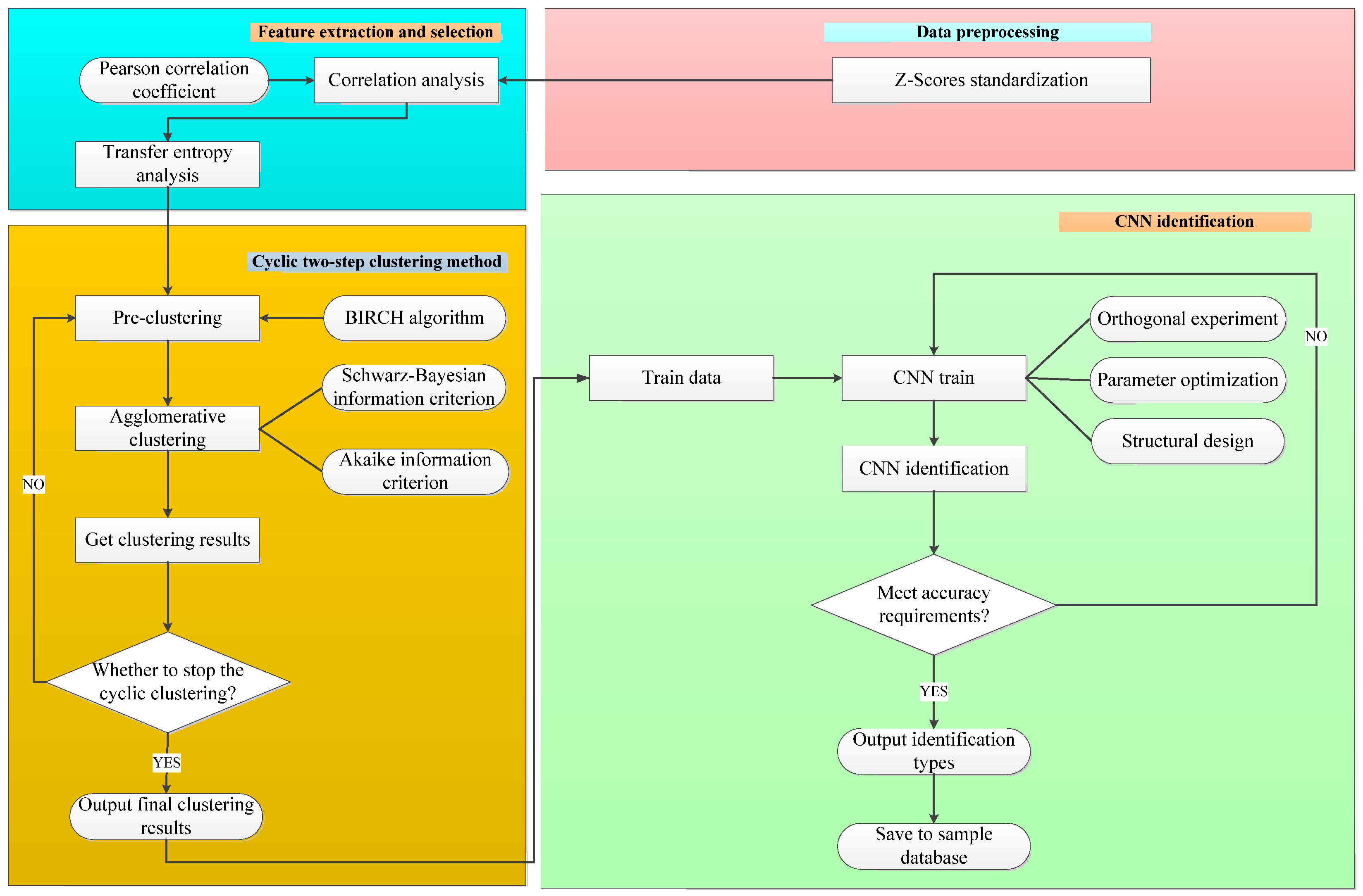
The CTSC-CNN method is composed of four parts: (1) data preprocessing; (2) feature selection; (3) CTSC method and (4) CNN identification. The framework of CTSC-CNN method is shown in Figure 1.

In the data processing part, the data of the control parameters and related variables are standardized by Z-Score standardization to reduce the effect of magnitudes on the data.

In the feature selection part, correlation analysis and transfer entropy analysis are performed on the preprocessed variables. Through calculating the Pearson correlation coefficient and transfer entropy, key variables are selected to successfully realize the reduction of the dimension.

In the CTSC analysis part, the optimal number of clustering is obtained by the Akaike information criterion (AIC) and the Schwarz Bayesian information criterion (BIC). The variables selected are clustered by the cyclic two-step clustering method to obtain more detailed clustering results with a fast and good effect.

In the CNN identification part, the dataset of clustering results is separated into a train set and a test set, respectively. The network hyperparameters in the CNN are optimized by means of quasi-orthogonal experiments.

2.1. Data Preprocessing

Differences in order of magnitude cause variables of larger magnitude to dominate the dataset, making their iterative convergence slow. Therefore, the data needs to be preprocessed to eliminate the effect of different magnitudes on different samples. Z-Scores standardization is carried out to reduce the effect of dimensions, resulting in a converted data mean value of 0 and a standard deviation of 1, as shown in Equation (1).

$$x_{ij}^{*}=\left\{\begin{array}{c}\frac{x_{ij}-\stackrel{-}{x_j}}{S_j}\hspace{1em} S_j\ne 0\\ \\ 0\hspace{1em}\hspace{1em}\hspace{1em}{S}_j=0\end{array}\right. \left(\genfrac{}{}{0pt}{}{i=\mathrm{1,2},\cdots ,\mathrm{n}}{j=\mathrm{1,2},\cdots ,\mathrm{n}}\right)$$

(1)

where $\overline{x_j}$ is the mean of the data and $S_j$ is the standard deviation of the data.

2.2. Feature Selection

In practical industrial big data applications, the correlation of variables may be low due to the influence of information flow between the time series, so it is limited to only considering the correlation. Combined with expert experience, a feature selection method based on correlation analysis and transfer entropy analysis is selected in this paper, which effectively solves the problem.

2.2.1. Correlation Analysis

Correlation analysis explores the degree and direction of the correlation of variables to study whether there is a certain dependency between variables. The study of correlation analysis is mainly about the degree of closeness between each two variables, which is a statistical method to study random variables. The correlation between variables is analyzed by using the Pearson correlation coefficient in this paper [13].

2.2.2. Transfer Entropy Analysis

The concept of transfer entropy comes from information theory, which measures the direction of information flow between two time series [14]. It essentially measures the degree to which the time series deviate from the Markov properties [15]. Transfer entropy is robust to data selection and effective for both linear and nonlinear relationships. The generalized Markov property can be expressed as $p\left(y_{t+1}|y_t^{\left(m\right)}\right)=p\left(y_{t+1}|y_t^{\left(m\right)},i_t^{\left(n\right)}\right)$. That is, the current state of a variable has nothing to do with anything else but its own state. The calculation equation of transfer entropy is shown in Equation (2) [16,17].

$$T_{I\to Y}\left(m,n\right)=\sum p\left(y_{t+1}|y_t^{\left(m\right)},i_t^{\left(n\right)}\right)\log \frac{p\left(y_{t+1}|y_t^{\left(m\right)},i_t^{\left(n\right)}\right)}{p\left(y_{t+1}|y_t^{\left(m\right)}\right)}$$

(2)

where I and Y represent the time series with order n and m Markov properties, respectively. y_t is the state or value of the Y sequence at time t, y_t^(m) = (y_t, …, y_t−m+1), i_t^(l) = (i, …, i_t−n+1). T_I→Y measures the flow of information from I to Y. P is the probability distribution. It is assumed that the chemical process variable is a first-order Markov process; that is, the parameters m and n are both set to 1 [18]. Furthermore, the probability distribution used in the above calculation is based on an empirical distribution.

2.3. CTSC Method

2.3.1. Cyclic Two-Step Clustering Method

The TSC method can automatically determine the optimal number of clustering, which is quite different from the traditional clustering methods. It can be used to solve the uncertain clustering problem of continuous data and discrete data and is suitable for clustering large data. Two-step clustering is separated into two stages. The first stage is called pre-clustering. The data points are processed one by one using the clustering tree growth theory in the BIRCH (Balanced Iterative Reducing and Clustering using Hierarchies) algorithm. When processing data points, the clustering tree is continuously updated by a set of split leaf nodes, forming many small sub-clusters. In the second stage, the clustering results of the first stage are used for clustering again with small clusters merged and grouped. The TSC is based on the combination of the two stages, which has an accurate clustering effect and good scalability. The similarity and dissimilarity between data individuals are calculated using the Euclidean distance function [19].

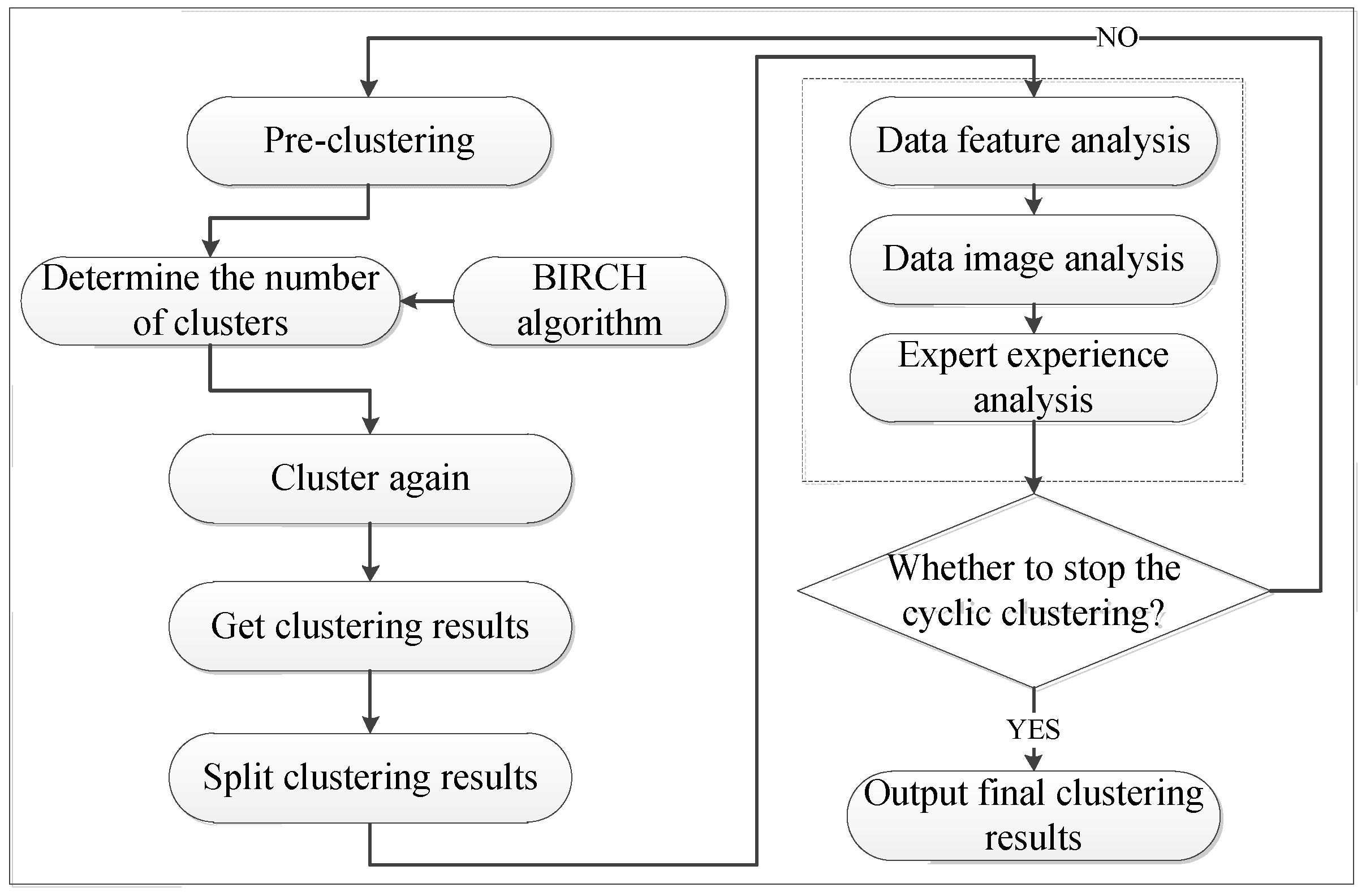
After one cycle of clustering, the classifications with obvious features are separated, but the obtained clustering results are not detailed enough. In this paper, a cyclic two-step clustering method is innovatively proposed, in which the obtained clustering results are further clustered in detail. The results of previously unknown types of abnormal conditions are thus further divided. The CTSC method is shown in Figure 2. The criteria for stopping the cycle include image analysis of the data, feature analysis of the data, and expert experience analysis, where the feature analysis of the data includes minimum value, maximum value, range, variance, mean, and standard deviation. When the stop rule is met, the clustering stops and the final clustering result is output. Otherwise, the cycle continues clustering.

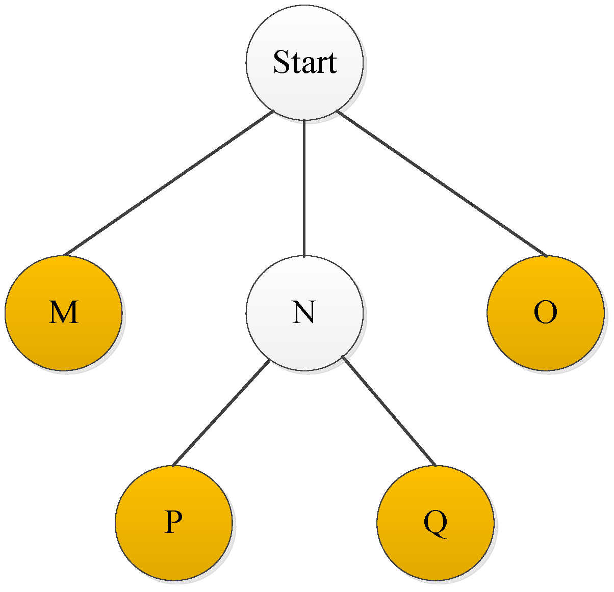
The results of CTSC method are represented in the form of tree diagram, where the nodes represent the clustering results of each step. When the node satisfies the cyclic clustering requirement, the tree diagram continues to grow with child nodes; otherwise, the tree diagram stops growing. For example, a simple tree diagram structure is shown in Figure 3. In the first clustering step, three clustering results are obtained, including Class N, Class M, and Class O. Among them, Class M and Class O do not satisfy the rule to continue cyclic clustering and therefore stop growing. Class N satisfies cyclic clustering and then continues to grow. Class N is clustered by a two-step clustering method again, resulting in classes P and Q. Class P and Class Q do not satisfy the rule to continue cyclic clustering and so stop growing. The final clustering results in 4 classes, which are Class Q, Class P, Class M, and Class O.

2.3.2. Kmeans Clustering Method

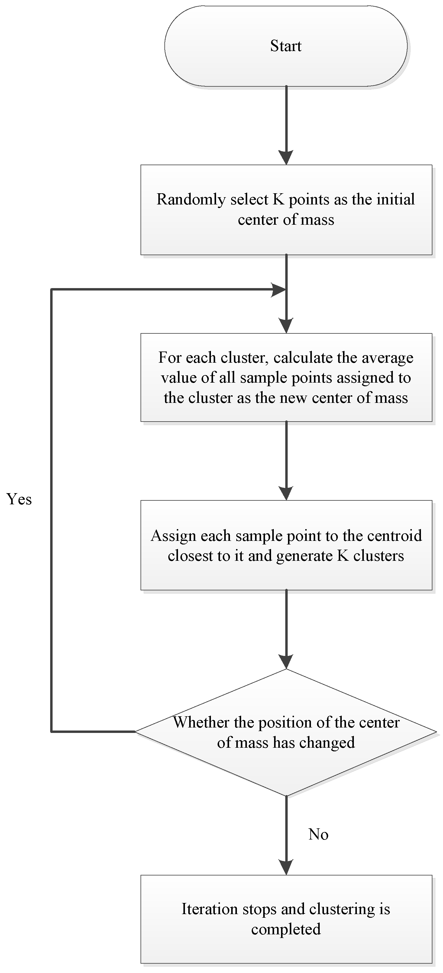
The Kmeans clustering algorithm is one of the commonly used clustering algorithms, which has the characteristics of simplicity, scalability, and so on. It is generally applied in many fields such as pattern identification, image processing, artificial intelligence, and bioengineering. The calculation process [7] of this clustering algorithm is shown in Figure 4. The observed objects are initially classified, and then adjusted to get the final classification. In this paper, the Kmeans clustering method is compared with the innovative CTSC method to illustrate the advantages of the CTSC method.

2.4. CNN Based Learning Process

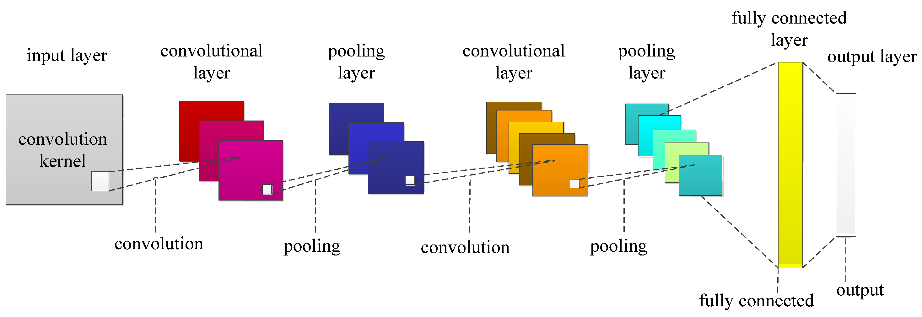
Convolutional neural networks occupy a very important position in deep neural networks and have been widely used in various fields. Convolutional neural networks were first proposed at the end of the 20th century by LeCun et al. After that, they developed rapidly with various variants emerging one after another. The biggest characteristic of a CNN is that it can automatically capture the higher-dimensional and more abstract features of the original input data layer by layer without specific prior knowledge than traditional neural networks. After obtaining the final abstracted features, the Softmax algorithm can be used to accurately classify multiple different categories. Figure 5 shows a typical CNN structure. Convolutional modules consist of an input layer, an output layer, a fully connected layer, pooling layers, and convolutional layers. These modules are able to capture the features of the original input data layer by layer, which are abstract to higher layers. The fully connected layer is generally in the previous layer of the network output layer, and its role is to perform regression or classification tasks.

A CNN is a network model that replaces the general multiplication operation in neural networks with convolution operations. The convolution operation is inspired by the visual cortex of animals. The convolutional layer has improved sparse connections and weight sharing in comparison with traditional neural networks. The weight sharing promotes the ability of each convolutional kernel to extract the same feature information from different input data during batch processing [20], which does not change with input data. A convolution kernel can perform element-wise multiplication and summation on the input matrix in the receptive field and add up the deviation. The convolution kernel is then moved by the stride until all regions of the input signal are computed. Equation (3) shows the convolution operation.

$$x_j=c_j^i\ast x_{j-1}+b_j^i$$

(3)

where ∗ represents the convolution operation, x_j−1 represents the output data of the j−1th layer, $c_j^i$ represents the ith convolution kernel of the jth layer, and $b_j^i$ represents the corresponding bias.

The CNN is composed of two basic layers: convolutional layers (feature extraction layers) and pooling layers (feature mapping layers). In the convolutional layer, the input of each neuron is connected to the local area of the previous feature for extracting local features and maintaining the relative positional relationship of the features. The pooling layer is composed of multiple features. Each feature domain is a plane. All neurons on the plane have equal weights, so that the feature plane has displacement invariance [21]. The operating principle of convolutional and pooling layers is described in detail below.

The input of the convolutional layer is the feature domain obtained by the previous layer [22]. When accepting the input feature, each convolution kernel in the convolutional layer has a limited range. The domain in this range is subjected to the convolution operation. If the convolutional layer has r convolution kernels, then r output feature domains are obtained. This is true for each input feature domain. Assuming the input is X, the output of the convolutional layer of a P × Q matrix can be calculated by Equation (4).

$$l_{i,j}^r=\theta \left({\left(W^r\ast X\right)}_{i,j}+b_r\right)$$

(4)

where $l_{i,j}^r$ is the value of the rth feature domain at the coordinate (i,j) obtained by the rth convolution kernel of the input domain, (i = 1, 2,…, P − z + 1, j = 1, 2,…, Q − z + 1). W_r∈R_z is the weight vector representing the rth convolution kernel. z is the size of the convolution kernel. b_r is the bias of the rth convolution kernel. θ(x) is the activation function, which is generally set as the Sigmoid or ReLU function.

Common pooling operations include average pooling and max pooling. By sampling the features at different positions of the input feature domain through the pooling layer, the size of the feature map obtained by convolution is reduced. The average pooling calculation is shown in Equation (5).

$$O_{i,j}=\frac{1}{z^2}\sum _{p,q=1}^z{l}_{\left(i-1\right)\times z+p,\left(j-1\right)\times z+q}$$

(5)

where O_i,j is the value of the output of the pooling layer at the coordinate (i,j), $l_{\left(i-1\right)\times z+p,\left(j-1\right)\times z+q}$ is the value of the input feature domain at the coordinate ((i − 1) × z + p, (j − 1) × z + q), and z is the pooling size [23].

At the end of the CNN, fully connected layers and classifiers are trained for classification. The fully connected layer uses a fully connected neural network [24] in this paper. The one-dimensional vector constructed from all the values in the feature domain obtained by the previous layer is used as the input of the fully connected neural network. The dot product of the input vector and the weight vector is calculated with the bias added. The results are classified by the Sigmoid function in the output layer or the Softmax classifier. In this paper, early stopping is added to prevent overfitting when training and testing data.

3. Industrial Applications

In order to verify the effectiveness of the CTSC-CNN method, an industrial application was performed on a catalytic cracking unit to identify the abnormal operating conditions in industrial production.

3.1. Process Description

The petroleum refining industry is one of the most basic industries of the national economy, which affects all aspects of people’s lives. Petroleum refining not only powers the transportation industry, but also provides raw material for other chemical plants. According to statistics, oil and its derivatives produced by petroleum refining can meet about 40% of the total global energy demand.

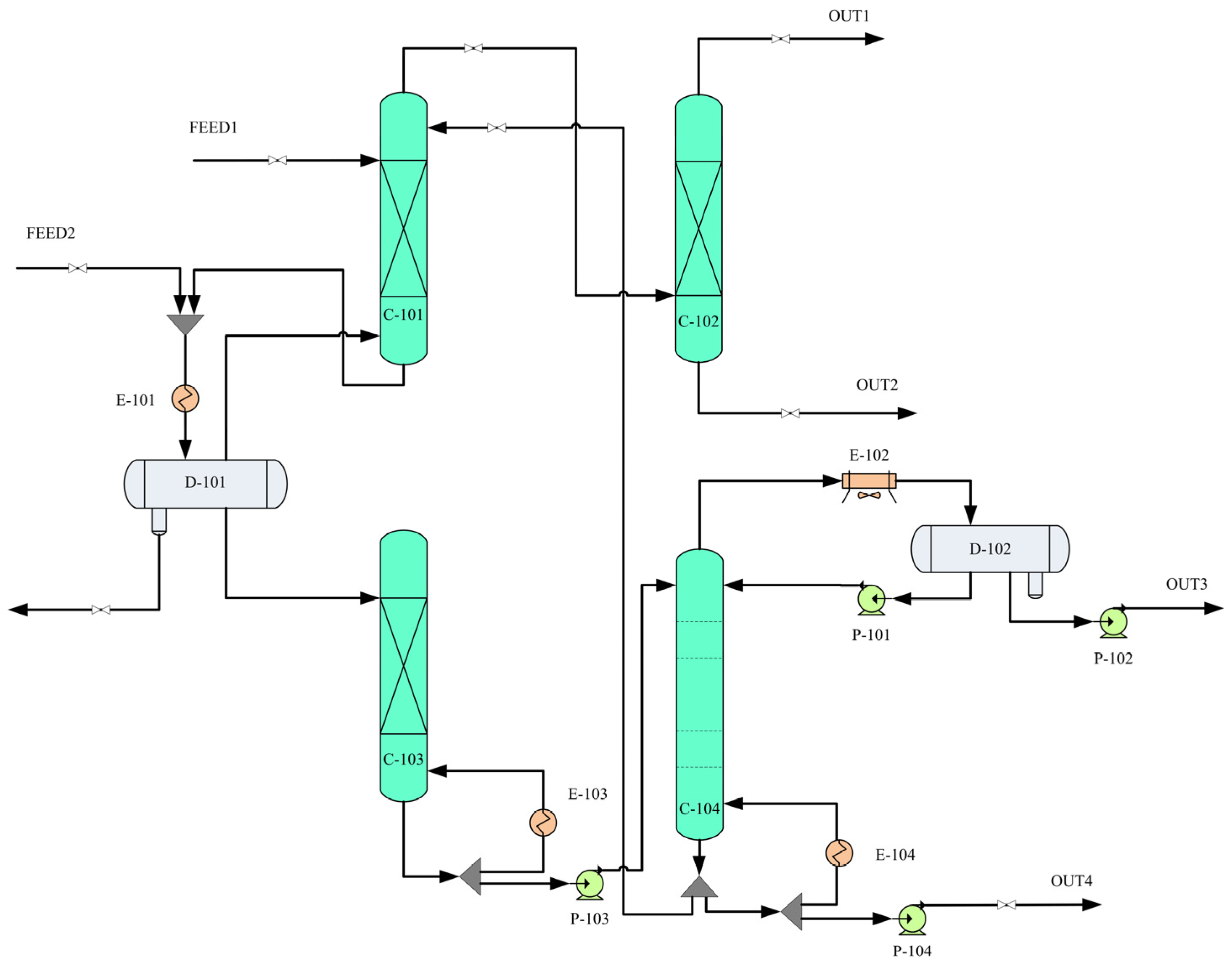
The catalytic cracking process has a harsh operating environment and complex structure, resulting in several unplanned shutdowns and abnormal operating conditions. The absorption stabilization system is an important part of the catalytic cracking process. Its main task is to separate the crude gasoline and high-pressure rich gas from the previous units into dry gas, liquefied gas, stabilized gasoline, and other products. At the same time, the content of C3 and the above heavy components in the dry gas are reduced as much as possible so that the quality of liquefied gas and stable gasoline is guaranteed to meet the product quality requirements. The state of the absorption process is important for the good operation of the whole device. The unknown operating conditions of the absorption stabilization system are mainly hidden in the temperature change, so the temperature is selected for key monitoring. According to the 347,520 operational observation data in two years, the abnormal operating conditions of the return temperature of the reboiler at the bottom of the desorption tower are identified. The entire system has 500 variables, which were collected every 3 min. Collection times are the same for different parts of the process system. The identification of abnormal operating conditions is meaningful for both the improvement of economic benefits and the long-term stable operation of the equipment.

The operation of the desorption tower has a great influence on the operation of the absorption stabilization system. Excessive desorption will not only cause the liquid level of the condensing oil tank to rise, but also lead to the waste of the heat source of the desorption tower and a large amount of desorption gas re-entering the air cooling and water cooling. In this situation, the load of the absorption tower and the energy consumption of the device will increase greatly. On the contrary, insufficient desorption will cause the pressure of the stabilization tower to be super high and affect the normal operation of the stabilization tower. The desorption effect has a great relationship with the return temperature of the reboiler of the desorption tower, and the control of this temperature is realized by adjusting the heat source control valve.

Figure 6 shows the flow chart of the absorption stabilization system of the catalytic cracking unit. The system includes absorption tower C-101, desorption tower C-103, reabsorption tower C-102, stabilization tower C-104, and so on. The crude gasoline and high-pressure rich gas in the previous process are separated into dry gas, liquefied gas, stabilized gasoline, and other products. FEED1 is crude gasoline and FEED2 is high-pressure rich gas. OUT1 represents dry gas, OUT2 represents rich absorption oil, OUT3 represents liquefied gas, and OUT4 represents stable gasoline.

3.2. Data Preprocessing

There are many variables in the FCC absorption stabilization system. Too many variables will make data analysis difficult. Only the variables related to the return temperature of the bottom reboiler in the desorption tower (T1) are considered in this paper. Combined with mechanism analysis, process knowledge, and practical work experience, 18 variables were selected through communication with field experts. These 18 variables were standardized with Z-Scores standardization. The standard deviation of the converted data was 1 and the mean value was 0.

3.3. Feature Selection of T1

The Pearson correlation coefficient analysis and transfer entropy analysis explored the relationship and properties between variables [25], and this could be used for feature selection. It was the basic work before data mining and has been widely used in research [26].

Table 1. Main variables related to T1.

Variables	Symbol Description	The Pearson Correlation Coefficient Value with T1	The Transfer Entropy Value with T1
T1	Return temperature of the bottom reboiler in the desorption tower	1.000	0
F1	Outlet flow at the top of the desorption tower	−0.093	0.000412
L1	Liquid level of the oil and gas separator at the outlet of the air compressor	0.461	0.000257
L2	Liquid level at the bottom of the absorption tower	0.622	0.000258
L3	Liquid level at the bottom of the stabilization tower	0.497	0.000407
L4	Liquid level of the reflux tank at the top of the stabilization tower	0.042	0.000563
L5	Liquid level at the bottom of the reabsorption tower	0.699	0.000517
P1	Pressure at the top of the desorption tower	0.672	0.000218
P2	Pressure at the top of the reabsorption	0.821	0.000280
T2	Temperature at the top of the absorption tower	0.088	0.000591
T3	Shell-side outlet temperature of the feed heat exchanger of the desorption tower	0.519	0.000475
T4	Temperature at the top of the stabilization tower	0.131	0.000219
T5	Temperature at the bottom of the stabilization tower	0.133	0.000223
T6	Catalytic dry gas temperature	0.179	0.000461
T7	Shell-side outlet temperature of the bottom reboiler of the stabilization tower	0.781	0.000138
T8	Shell-side outlet temperature of the bottom reboiler of the desorption tower	0.911	0.002282
T9	Shell side outlet temperature of the reboiler in the middle section of the desorption tower	0.709	0.001272
L6	Liquid level at the bottom of the desorption tower	0.533	0.000763

lists the Pearson correlation coefficients and transfer entropy values of 18 variables with T1.

Through the correlation analysis and transfer entropy analysis in Table 1, the correlation between each variable and T1 could be intuitively reflected. After feature selection, there were eight highly correlated variables, as shown in

Table 2. Variables after feature selection.

Variables	Symbol Description	The Pearson Correlation Coefficient Value with T1	The Transfer Entropy Value with T1
T1	Return temperature of the bottom reboiler of the desorption tower	1.000	0
L5	Liquid level at the bottom of the reabsorption tower	0.699	0.000517
P2	Pressure at the top of the reabsorption	0.821	0.000280
L2	Liquid level at the bottom of the absorption tower	0.622	0.000258
P1	Pressure at the top of the desorption tower	0.672	0.000218
T8	Shell-side outlet temperature of the bottom reboiler of the desorption tower	0.911	0.002282
T9	Shell side outlet temperature of the reboiler in the middle section of the desorption tower	0.709	0.001272
L6	Liquid level at the bottom of the desorption tower	0.533	0.000763

. Through feature selection, the data are effectively reduced in dimensionality. For the identification of the CTSC-CNN model in this paper, it was very necessary to reduce the dimension of data variables. Too many variables would cause a waste of computing resources, and effective clustering results would not be obtained.

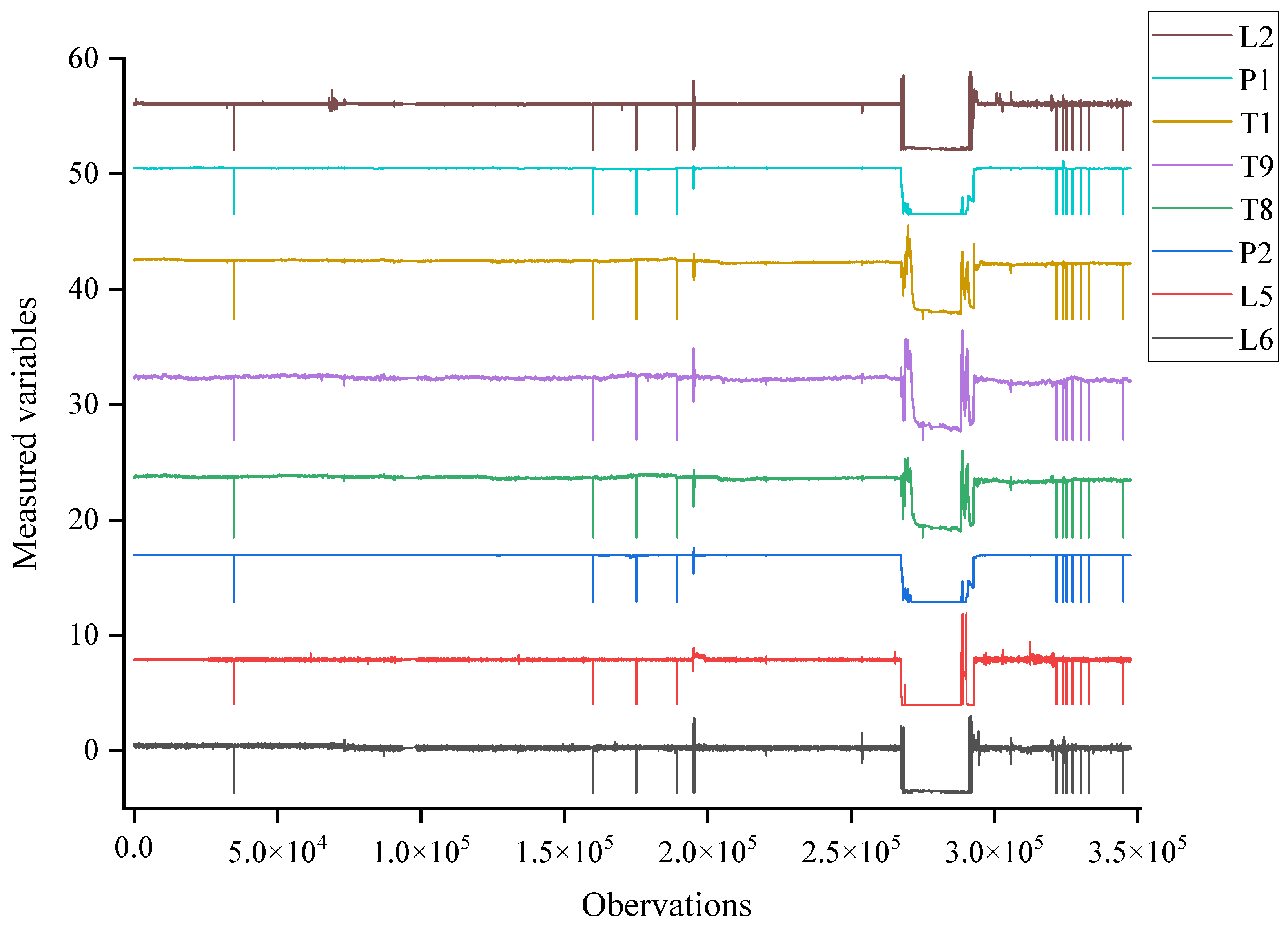
The standardized data of these eight variables are shown in Figure 7. It can be seen that the variables after feature selection have a high correlation with T1.

3.4. Cyclic Two-Step Cluster Analysis

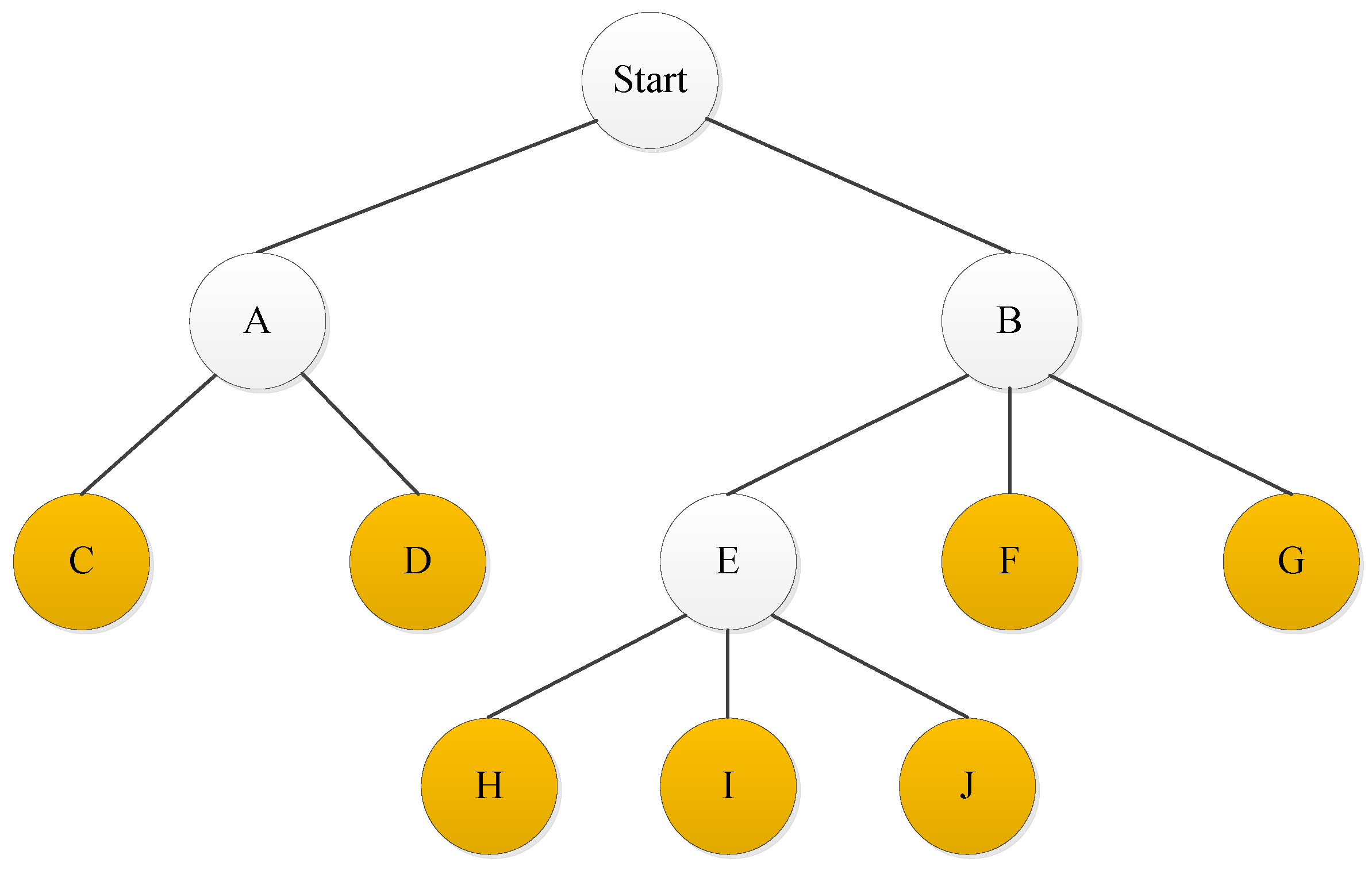
The resulting eight variables were clustered using the cyclic two-step clustering method. The tree diagram of the clustering results is shown in Figure 8. In the first clustering step, two clustering results were obtained, which were Class B and Class A. Class B and Class A satisfied the criteria to continue cyclic clustering, so the tree continued to grow. Class A was clustered by the two-step clustering method again, resulting in classes C and D. Class C and Class D did not satisfy the criteria to continue cyclic clustering and stopped growing. Class B was clustered by the two-step clustering method, resulting in classes E, F, and G. Class F and Class G did not satisfy the criteria to continue cyclic clustering and stop growing. Class E satisfy the continuous cycle clustering criteria and continued to grow. Class E was clustered by the two-step clustering method, resulting in Class H, Class I, and Class J. Class J, Class I, and Class H did not satisfy the criteria to continue cyclic clustering and stopped growing. The final clustering resulted in seven classes, which were Class J, Class I, Class H, Class G, Class F, Class D, and Class C.

The size of each class in the final cyclic two-step clustering results is shown in

Table 3. The cluster size of each class of the cyclic two-step clustering results.

Clustering Name	Operating Condition Name	Cluster Size	The Number of Observations
Class C	Abnormal operating condition 1	2.29%	7958
Class D	Abnormal operating condition 2	5.11%	17,749
Class F	Normal operating condition 1	25.20%	87,856
Class G	Normal operating condition 2	66.49%	231,056
Class H	Abnormal operating condition 3	0.08%	294
Class I	Abnormal operating condition 4	0.27%	941
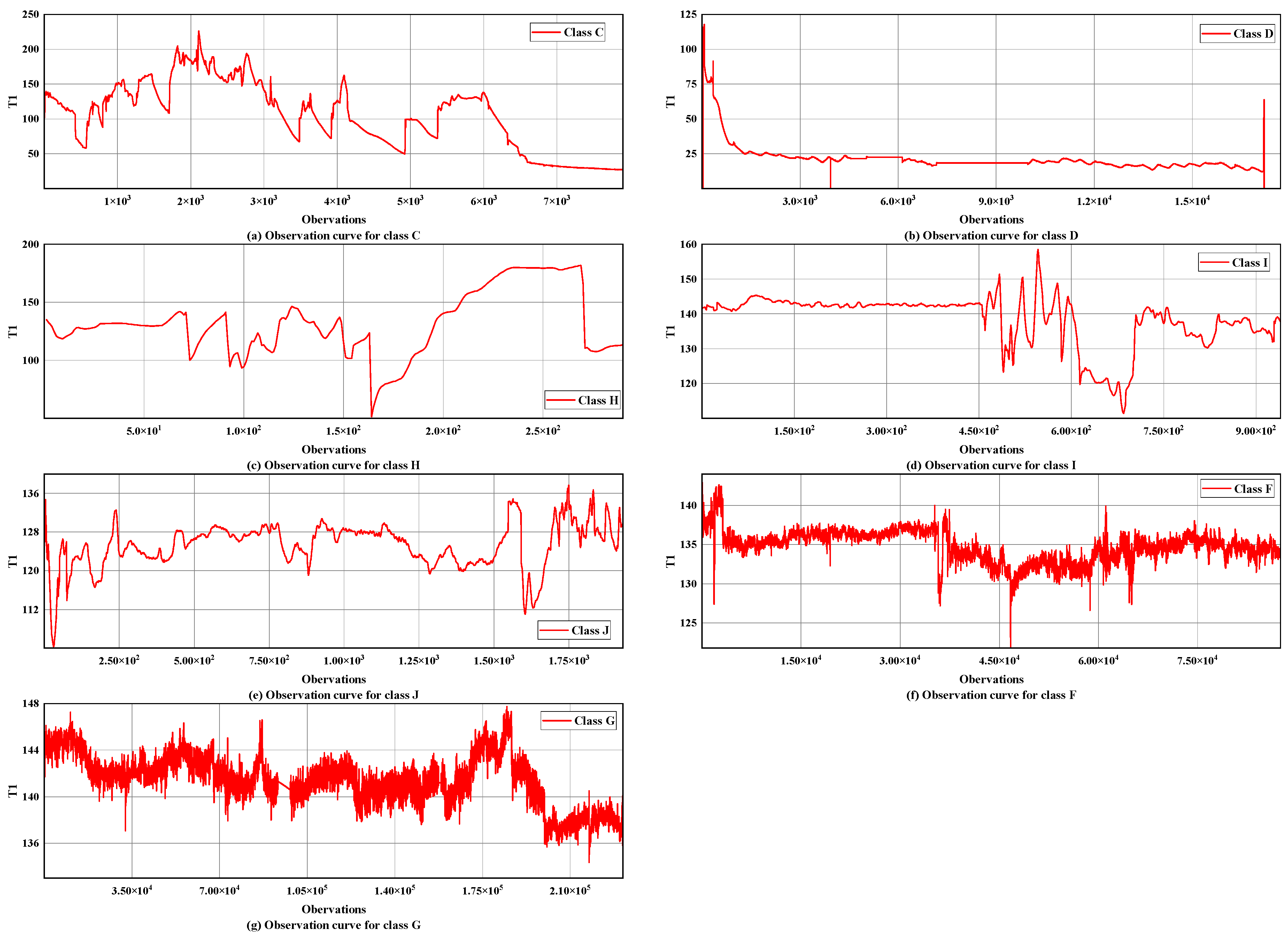
Class J	Abnormal operating condition 5	0.56%	1936

. There were seven types of clusters in the cyclic two-step clustering results. The normal value range of T1 was around 136. The numerical properties of Class F fluctuated within the normal range, so it was normal operating condition 1, with 87,856 observations clustered in this class. The numerical properties of Class G also fluctuated within the normal range. Class G was thus normal operating condition 2, with 231,056 observations clustered in this class. Class F and Class G were two different types of normal operating conditions. Changes in the composition of the feedstock and differences in feed conditions could have resulted in different types of normal operating conditions. The numerical characteristics of Class H, Class D, Class C, Class J, and Class I had a larger fluctuation range in comparison with the normal value. Class C was abnormal operating condition 1 with a total of 7958 observations. Class D was abnormal operating condition 2, with a total of 17,749 observations. Class H was abnormal operating condition 3, with a total of 294 observations. Class I was abnormal operating condition 4, with a total of 941 observations. Class J was abnormal operating condition 5 with a total of 1936 observations. The data feature analysis of these classes is shown in

Table 4. The data feature analysis of the cyclic two-step clustering classes.

Clustering Name	Maximum Value	Minimum Value	Range	Mean	Variance	Standard Deviation
Class C	226.056	26.840	199.216	104.179	2310.441	48.067
Class D	117.901	0.000	117.901	20.840	126.461	11.245
Class F	142.891	121.983	20.908	134.775	3.980	1.995
Class G	147.749	134.285	13.464	141.470	4.343	2.084
Class H	181.708	51.343	130.365	131.192	744.647	27.288
Class I	158.494	111.448	47.046	138.466	54.217	7.363
Class J	137.708	104.323	33.385	125.284	21.195	4.604

.

The observation curves of T1 in the CTSC classes are shown in Figure 9. It can be seen that the cyclic two-step clustering achieved good clustering results. From Table 3 and Table 4, Figure 9, and the overall changes in T1 data, combined with expert analysis and numerical analysis, Class F and Class G were normal operating conditions. Class C was an abnormal operating condition due to the startup and shutdown of the device. Class D was an abnormal operating condition caused by meter damage and meter calibration. Class H, Class I, and Class J were three kinds of abnormal operating conditions caused by other reasons.

3.5. Comparison with Kmeans Clustering Method

For better comparison between different clustering methods, the K value of the Kmeans clustering method was set to 7. The size of each class in the Kmeans clustering results is shown in

Table 5. The cluster size of each class of the Kmeans clustering results.

Clustering Name	Operating Condition Name	Cluster Size	The Number of Observations
Class 1	Abnormal operating condition 1	0.72%	2508
Class 2	Abnormal operating condition 2	0.31%	1063
Class 3	Abnormal operating condition 3	4.97%	17,266
Class 4	Abnormal operating condition 4	0.25%	866
Class 5	Abnormal operating condition 5	0.34%	1179
Class 6	Normal operating condition 1	92.59%	321,782
Class 7	Abnormal operating condition 6	0.82%	2856

. There were seven types of clusters in the Kmeans clustering results. The data feature analysis of the Kmeans clustering classes is shown in

Table 6. Data feature analysis of the Kmeans clustering classes.

Clustering Name	Maximum Value	Minimum Value	Range	Mean	Variance	Standard Deviation
Class 1	134.303	35.256	99.047	74.369	409.257	20.230
Class 2	142.499	62.916	79.584	113.531	299.100	17.295
Class 3	63.753	0.000	63.753	19.098	27.328	5.228
Class 4	150.874	81.400	69.474	106.253	234.441	15.311
Class 5	118.902	26.840	92.062	31.893	66.267	8.140
Class 6	181.708	93.332	88.376	139.536	15.075	3.883
Class 7	226.056	99.636	126.420	152.448	595.944	24.412

. As can be seen from Table 5 and Table 6, the numerical properties of Class 6 fluctuated within the normal range. Therefore, Class 6 was normal operating condition 1, with 321,782 observations clustered in this class. The numerical characteristics of Class 1, Class 2, Class 3, Class 4, Class 5, and Class 7 had a larger fluctuation range in comparison with the normal value. Class 1 was abnormal operating condition 1 with a total of 2508 observations. Class 2 was abnormal operating condition 2, with a total of 1063 observations. Class 3 was abnormal operating condition 3, with a total of 17,266 observations. Class 4 was abnormal operating condition 4, with a total of 866 observations. Class 5 was abnormal operating condition 5 with a total of 1179 observations. Class 7 was abnormal operating condition 6 with a total of 2856 observations.

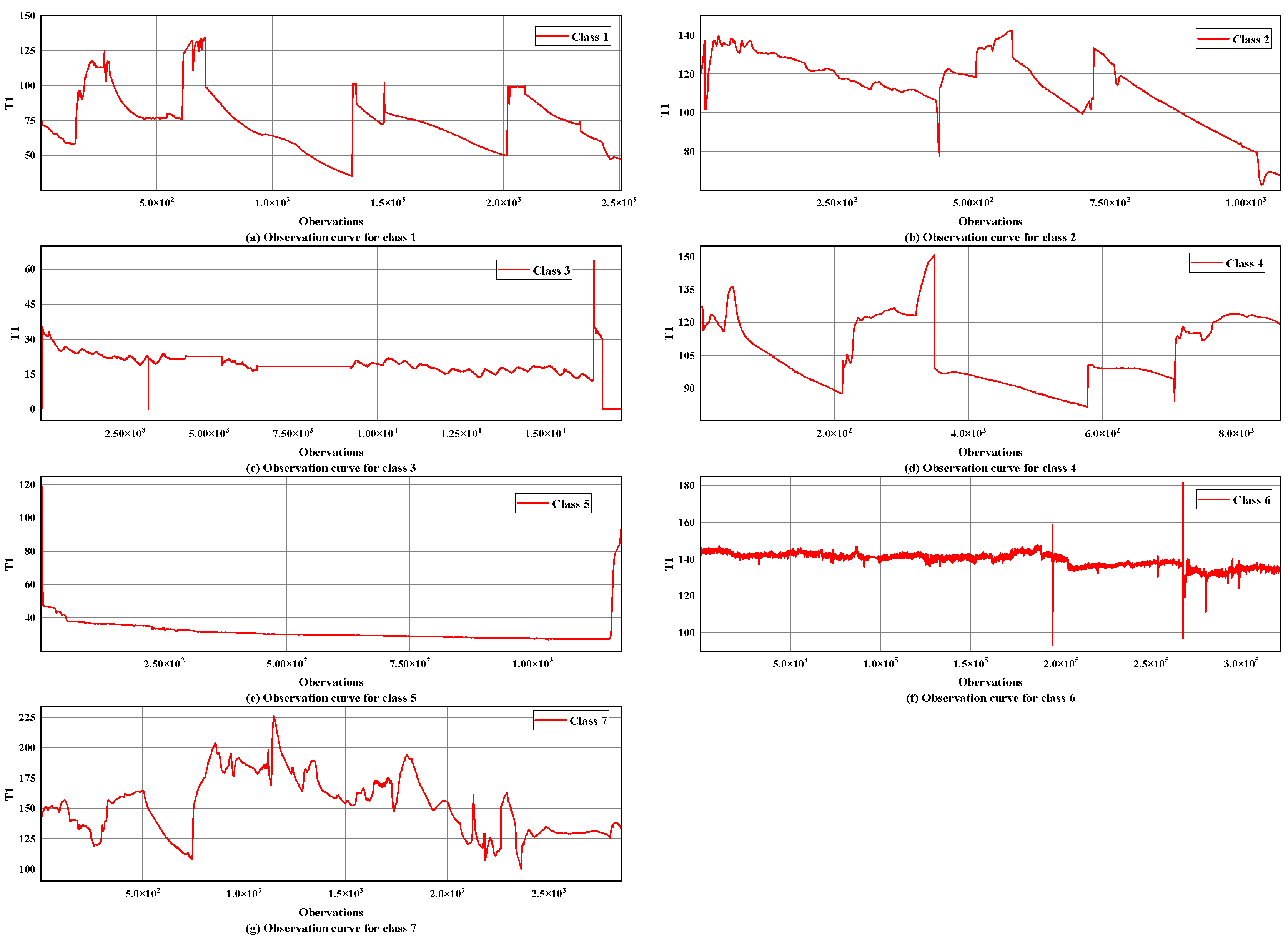
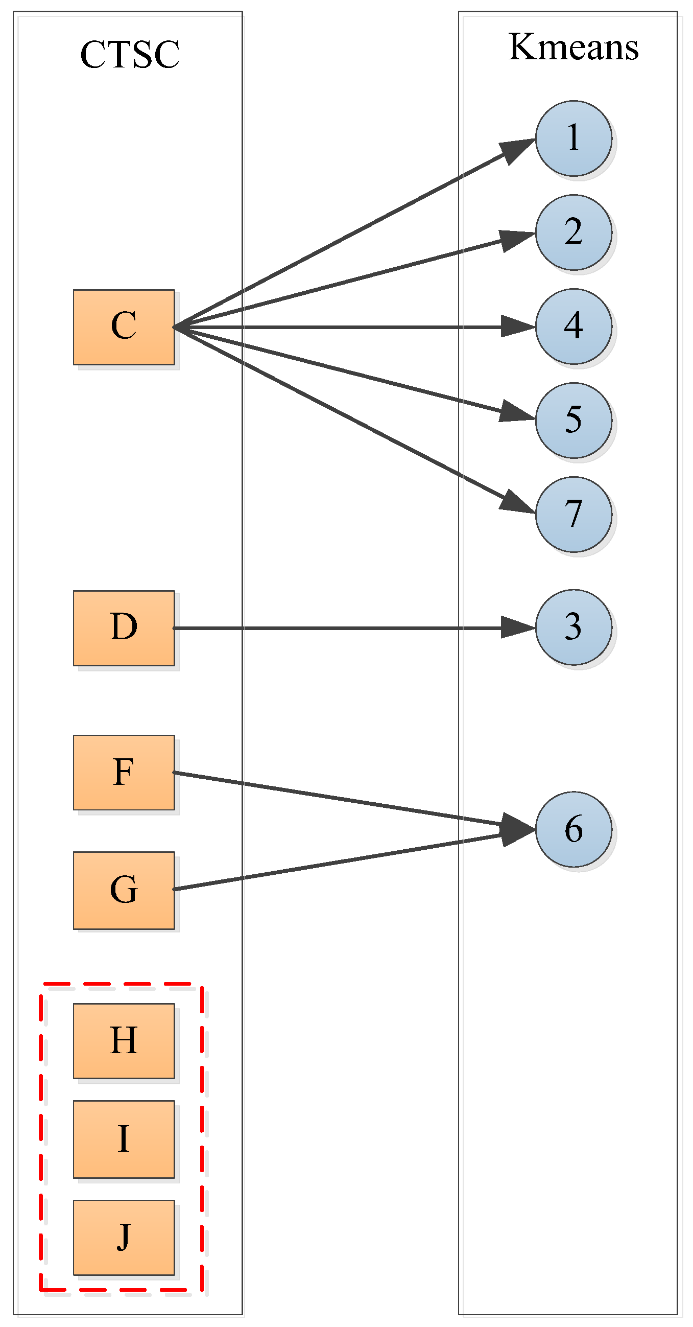
The observation curves of T1 in the Kmeans clustering classes are shown in Figure 10. From Table 5 and Table 6, Figure 10, and the overall changes in T1 data, combined with expert analysis and numerical analysis, Class 6 was a normal operating condition. Class 1, Class 2, Class 4, Class 5, and Class 7 were abnormal operating conditions due to startup and shutdown of the device. Class 3 was an abnormal operating condition caused by meter damage and meter calibration. The comparison of CTSC clustering results and Kmeans clustering results is shown in Figure 11.

As shown in Figure 11, the CTSC clustering method proposed in this paper has had a better performance. Class 1, Class 2, Class 4, Class 5, and Class 7 obtained from the Kmeans clustering results were abnormal conditions clustered before and after startup and shutdown, which were all included in the Class C of the CTSC clustering results. In the CTSC clustering results, the normal operating conditions were classified as Class F and Class G. The normal value range of T1 was around 136. In the Kmeans clustering results, only Class 6 represented the normal operating condition, but its maximum value was 181.708, minimum value is 93.332, and range is 88.376, indicating that a large number of abnormal operating condition data were clustered into the normal operating condition class. In addition, the three abnormal operating conditions of Class H, Class I, and Class J obtained from the CTSC clustering results were not effectively clustered in the Kmeans clustering results. From the comparison results, it can be clearly seen that the CTSC clustering method had an excellent clustering performance and was more suitable for the data-driven identification of abnormal operating conditions in actual industrial production.

3.6. Identification Result

The features of the CTSC clustered classes are identified in this section. The latent relationship between variables was deeply mined. The network learning effect was tested through the test set. The dataset had to be delimited before entering the network. The dataset was randomly sampled with a ratio of 2:8 and divided into a test set and a training set to better test the advantages and disadvantages of the network.

The V&V method was used to find the optimal model hyperparameters. Its steps were divided into two steps. The first step was to design the structure of the network model and verify whether the structure was reasonable and whether it conformed to the optimal design principle of the network through expert experience. The second step was to use the training set for network training and verify network performance through the test set. If it was not satisfactory, the network hyperparameters had to be readjusted. Otherwise, the adjustment was stopped. Through continuous testing, the CNN network structure and hyperparameters were finally determined as shown in

Table 7. CNN network structure and hyperparameter.

Input Variable Dimension	Pooling Layer 1 Size	Pooling Layer 2 Size	Fully Connected Layer Size
8	2	2	32

and

Table 8. CNN convolutional layer structure.

Convolutional Layer	Filter	Convolution Kernel
1	32	3
2	64	3
3	64	3
4	64	3
5	128	3
6	128	3

. The CNN structure contained six convolutional layers and two pooling layers. The optimization algorithm used was the Adaptive Moment Estimation algorithm. The error variation of the network was monitored by the Early Stopping method. When there was a downward trend in the training process, the iteration was stopped in time to ensure the accuracy of network identification. At the same time, a dropout layer was added to prevent the network from overfitting [27].

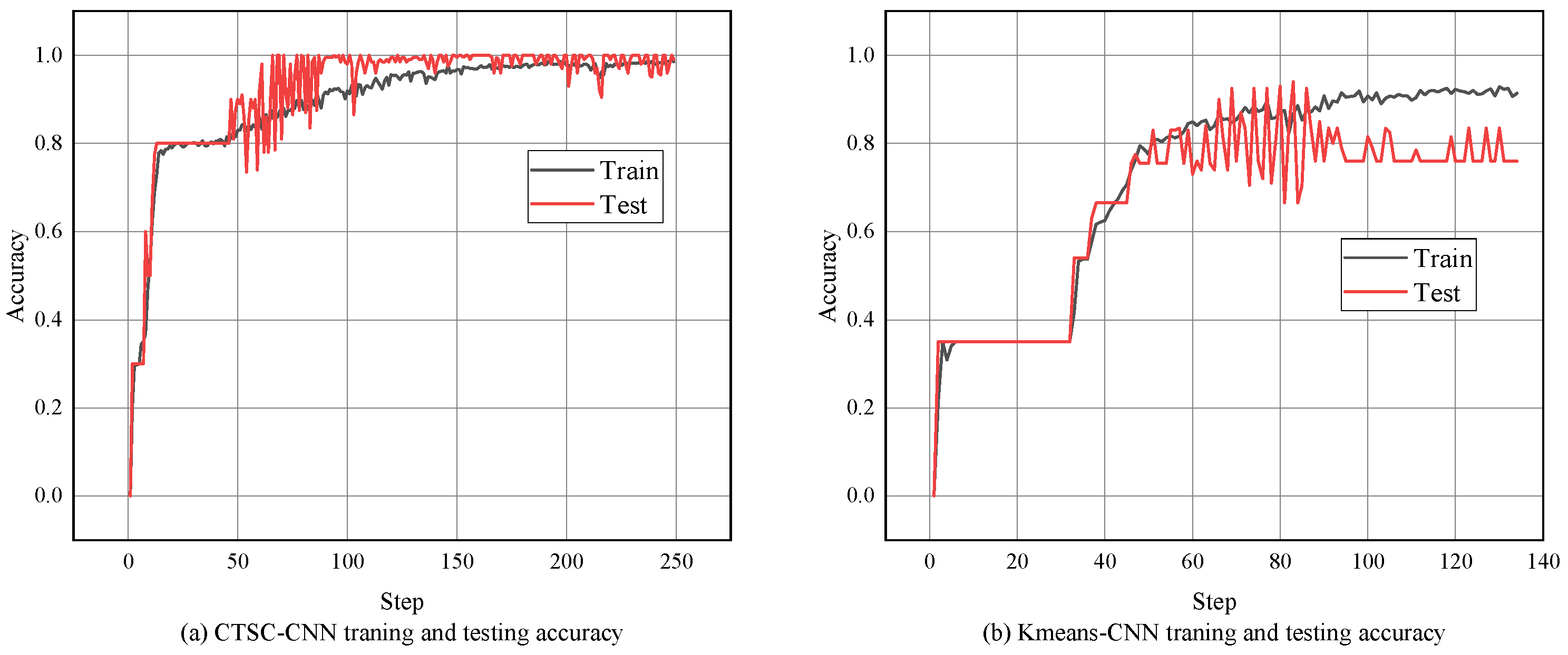
For comparison, Figure 12a,b shows the identification accuracy of CTSC-CNN and Kmeans-CNN, respectively. The accuracy rate of the CTSC-CNN model on test set finally reaches 99.0%, while the Kmeans-CNN model only reaches 76.0%. Compared with the Kmeans-CNN model, the CTSC-CNN model has higher identification accuracy, and the accuracy fluctuation during model training was smaller. The test set and training set-based results of the CTSC-CNN model had almost the same trend (rising smoothly with the increase of the number of iterations), proving the stability of the CTSC-CNN learner.

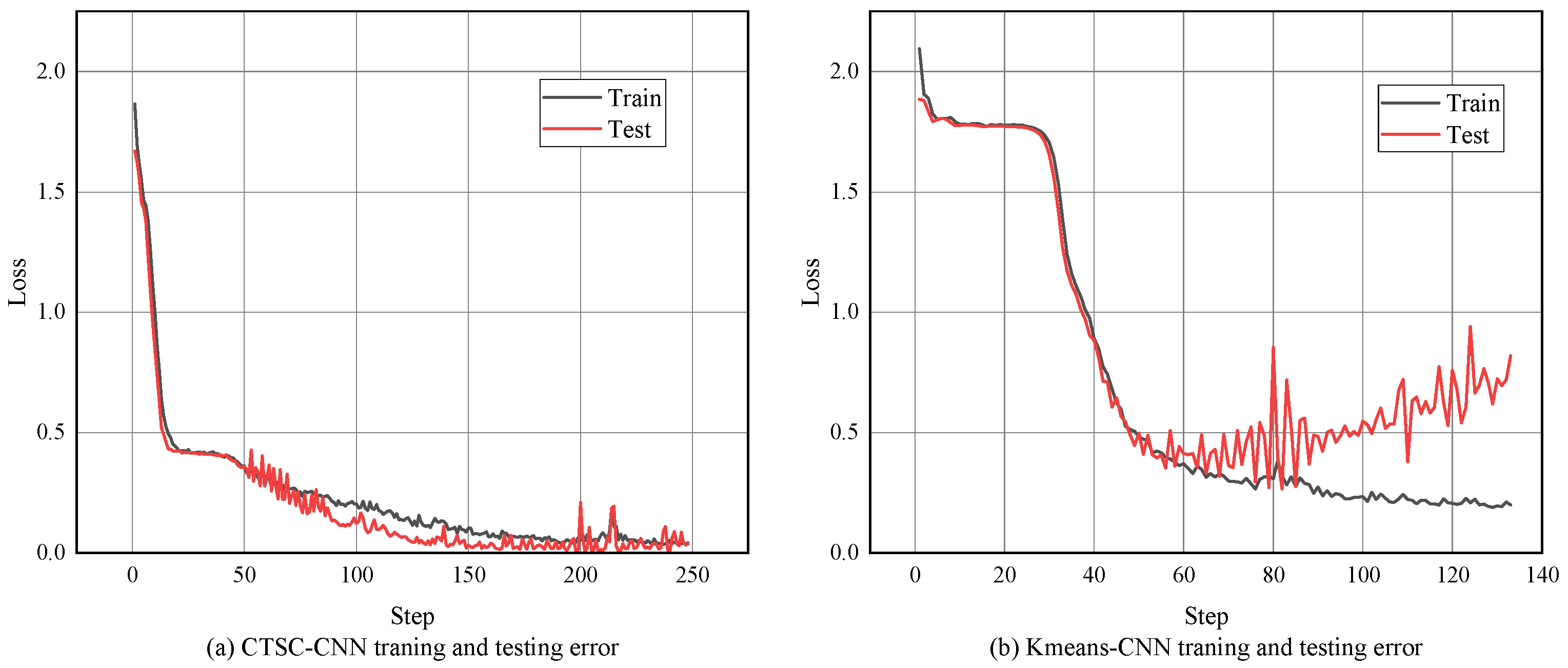
The CNN-based learning process in this paper included the mean square error loss function. Figure 13a,b shows the identification errors of CTSC-CNN and Kmeans-CNN, respectively. The final error of the CTSC-CNN model on test set was 0.04, while the final error of the Kmeans-CNN model on test set was 0.82. Compared with the Kmeans-CNN model, the error of the CTSC-CNN model decreased faster with the iteration, and was smaller and more stable in the later stage of the training process. At about 50 times, the learning efficiency of CTSC-CNN began to decline. After that, the error gradually stabilized.

From the comparison results, it can be seen that the CTSC-CNN method proposed in this paper had an excellent identification performance and had a very good identification effect on the abnormal operating conditions of the absorption and stabilization system of the catalytic cracking process. The identified normal operating conditions and abnormal operating conditions were stored in the operating condition sample database, which effectively realizes the rapid identification of unknown operating conditions.

4. Conclusions

In this work, a novel CTSC method was proposed and the CTSC clustering in catalytic cracking process was realized. After the optimal model parameters were obtained through the adjustment of the training set and test set, CTSC-CNN was comprehensively analyzed. The results are shown as follows:

(1) Through correlation analysis and transfer entropy analysis, eight variables were selected, such as the pressure at the top of the reabsorption, the shell-side outlet temperature of the bottom reboiler of desorption tower, and the liquid level at the bottom of the absorption tower.

(2) The comparison of CTSC clustering results and Kmeans clustering results demonstrated that the CTSC clustering method has an excellent clustering performance and was more suitable for data-driven identification of abnormal operating conditions in actual industrial production. The clustering results obtained by the CTSC clustering method were better, and the abnormal operating conditions of Class H, Class I, and Class J were further obtained by comparing the Kmeans clustering method.

(3) The accuracy of the CTSC-CNN model on the test set finally reached 99.0%, and its identification error reached as low as 0.04. The results indicate that the operating conditions were effectively identified by CTSC-CNN model.

The potential research directions in the future will include further optimization and improvement of the clustering algorithm to realize rapid and effective identification of abnormal conditions in industrial production and reduce the occurrence of safety accidents. The organic combination of the clustering method and the machine learning algorithm will be further studied to make a greater contribution to the realization of intelligent industrial production. In addition, the identification research of abnormal conditions will be combined with the root cause analysis of abnormal conditions, and the abnormal conditions will be labeled.

References

- Cai, W.; Deng, R.; Gao, C.; Wang, Y.; Ning, W.; Shu, B.; Chen, Z. Evaluation techniques for shale oil lithology and mineral composition based on principal component analysis optimized clustering algorithm. Processes 2023, 11, 958. [Google Scholar] [CrossRef]
- Ning, C.; Chen, M.; Zhou, D. Hidden Markov Model-Based Statistics Pattern Analysis for Multimode Process Monitoring: An Index-Switching Scheme. Ind. Eng. Chem. Res. 2014, 53, 11084–11095. [Google Scholar] [CrossRef]
- Wang, X.; Wang, X.; Wang, Z.; Qian, F. A novel method for detecting processes with multi-state modes. Control Eng. Pract. 2013, 21, 1788–1794. [Google Scholar] [CrossRef]
- Xie, X.; Shi, H. Dynamic Multimode Process Modeling and Monitoring Using Adaptive Gaussian Mixture Models. Ind. Eng. Chem. Res. 2012, 51, 5497–5505. [Google Scholar] [CrossRef]
- Wang, L.; Yang, C.; Sun, Y. Multimode Process Monitoring Approach Based on Moving Window Hidden Markov Model. Ind. Eng. Chem. Res. 2018, 57, 292–301. [Google Scholar] [CrossRef]
- Tan, J.P.; Yang, Z.J.; Cheng, Y.Q.; Ye, J.L.; Wang, B.; Dai, Q.Y. SRAGL-AWCL: A two-step multi-view clustering via sparse representation and adaptive weighted cooperative learning. Pattern Recognit 2021, 117, 107987. [Google Scholar] [CrossRef]
- Hong, J.; Qu, J.; Tian, W.D.; Cui, Z.; Liu, Z.J.; Lin, Y.; Li, C.K. Identification of unknown abnormal conditions in catalytic cracking process based on two-step clustering analysis and signed directed graph. Processes 2021, 9, 2055. [Google Scholar] [CrossRef]
- Guediri, A.; Hettiri, M.; Guediri, A. Modeling of a wind power system using the genetic algorithm based on a doubly fed induction generator for the supply of power to the electrical grid. Processes 2023, 11, 952. [Google Scholar] [CrossRef]
- Chen, W.Y.; Zhang, L.M. An automated machine learning approach for earthquake casualty rate and economic loss prediction. Reliab. Eng. Syst. Saf. 2022, 225, 108645. [Google Scholar] [CrossRef]
- Deng, L.; Zhang, Y.; Dai, Y.Y.; Ji, X.; Zhou, L.; Dang, Y.G. Integrating feature optimization using a dynamic convolutional neural network for chemical process supervised fault classification. Process Saf. Environ. Prot. 2021, 155, 473–485. [Google Scholar] [CrossRef]
- Jia, X.M.; Qin, N.; Huang, D.Q.; Zhang, Y.M.; Du, J.H. A clustered blueprint separable convolutional neural network with high precision for high-speed train bogie fault diagnosis. Neurocomputing 2022, 500, 422–433. [Google Scholar] [CrossRef]
- He, C.; Ge, D.C.; Yang, M.H.; Yong, N.; Wang, J.Y.; Yu, J. A data-driven adaptive fault diagnosis methodology for nuclear power systems based on NSGAII-CNN. Ann. Nucl. Energy 2021, 159, 108326. [Google Scholar] [CrossRef]
- Liu, Y.; Mu, Y.; Chen, K.; Li, Y.; Guo, J. Daily activity feature selection in smart homes based on Pearson correlation coefficient. Neural Process. Lett. 2020, 51, 1771–1787. [Google Scholar] [CrossRef]
- Benedetto, F.; Mastroeni, L.; Quaresima, G.; Vellucci, P. Does OVX affect WTI and Brent oil spot variance? Evidence from an entropy analysis. Energy Econ. 2020, 89, 104815. [Google Scholar] [CrossRef]
- Liu, N.; Wang, J.; Sun, S.L.; Li, C.K.; Tian, W.D. Optimized principal component analysis and multi-state Bayesian network integrated method for chemical process monitoring and variable state prediction. Chem. Eng. J. 2022, 430, 132617. [Google Scholar] [CrossRef]
- Schreiber, T. Measuring Information Transfer. Phys. Rev. Lett. 2000, 85, 461–464. [Google Scholar] [CrossRef]
- Shannon, C.E. A Mathematical Theory of Communication. Bell Syst. Tech. J. 2001, 5, 3–55. [Google Scholar] [CrossRef]
- Simon, B.; Thomas, D.; Franziska, J.P.; David, J.Z. RTransferEntropy-Quantifying information flow between different time series using effective transfer entropy. SoftwareX 2019, 10, 100265. [Google Scholar]
- Xue, W. Statistical Analysis and SPSS Application; China Renmin University Press: Beijing, China, 2017; pp. 269–272. [Google Scholar]
- Zhu, Z.J.; Li, D.M.; Hu, Y.; Li, J.S.; Liu, D.; Li, J.J. Indoor scene segmentation algorithm based on full convolutional neural network. Neural Comput. Appl. 2020, 2, 8261–8273. [Google Scholar] [CrossRef]
- Guo, S.; Yang, T.; Gao, W.; Zhang, C. A Novel Fault Diagnosis Method for Rotating Machinery Based on a Convolutional Neural Network. Sensors 2018, 18, 1429. [Google Scholar] [CrossRef] [PubMed]
- Song, Q.S.; Jiang, P. A multi-scale convolutional neural network based fault diagnosis model for complex chemical processes. Process Saf. Environ. Prot. 2022, 159, 575–584. [Google Scholar] [CrossRef]
- He, Y.F.; Liu, X.F.; Lu, X.L.; He, L.P.; Ma, Y.X.; Guo, X.; Yang, T. Modeling and Intelligent Identification of Axis Orbit for Rotating Machinery Based on the Convolution Neural Networks. J. Phys. Conf. Ser. 2021, 1746, 12011. [Google Scholar] [CrossRef]
- Guo, S.; Zhang, B.; Yang, T.; Lyu, D.Z.; Gao, W. Multitask Convolutional Neural Network with Information Fusion for Bearing Fault Diagnosis and Localization. IEEE Trans. Ind. Electron. 2020, 67, 8005–8015. [Google Scholar] [CrossRef]
- Edelmann, D.; Móri, T.F.; Székely, G.J. On relationships between the Pearson and the distance correlation coefficients. Stat. Probab. Lett. 2021, 169, 108960. [Google Scholar] [CrossRef]
- Qin, L.M.; Yang, G.; Sun, Q. Maximum correlation Pearson correlation coeffcient deconvolution and its application in fault diagnosis of rolling bearings. Measurement 2022, 205, 112162. [Google Scholar] [CrossRef]
- Li, Y.B.; Wan, H.; Jiang, L. Alignment subdomain-based deep convolutional transfer learning for machinery fault diagnosis under different operating conditions. Meas. Sci. Technol. 2022, 33, 55006. [Google Scholar] [CrossRef]
Figure 1.
The framework of the CTSC-CNN method.
Figure 2.
CTSC method flowchart.
Figure 3.
A simple tree diagram structure.
Figure 4.
Kmeans clustering algorithm calculation steps.
Figure 5.
Basic CNN structure.
Figure 6.
Flow chart of absorption stabilization system of catalytic cracking unit.
Figure 7.
The standardized data of 8 variables.
Figure 8.
The tree diagram after cyclic two-step clustering.
Figure 9.
The observation curves of the cyclic two-step clustering classes of T1.
Figure 10.
The observation curves of the Kmeans clustering classes of T1.
Figure 11.
Comparison of CTSC clustering results and Kmeans clustering results.
Figure 12.
Comparison of training and testing accuracy of CTSC-CNN (a) and Kmeans-CNN (b).
Figure 13.
Comparison of training and testing error of CTSC-CNN (a) and Kmeans-CNN (b).