Abstract
Wellbore leakage mostly occurs in structurally developed fractured formations. Analyzing the real-time leakage rate during the drilling process plays an important role in identifying the leakage mechanism and its rules on-site. Based on the principles of fluid mechanics and using Herschel-Bulkley (H-B) drilling fluid, by reasonably simplifying the drilling fluid performance parameters, fracture roughness characteristic parameters, pressure difference between the wellbore and formation, and the radial extension length of drilling fluid, the radial leakage model is improved to improve the calculation accuracy. Using the Euler format in numerical analysis to solve the model and with the help of numerical analysis software, the radial leakage law of this flow pattern in the fractures is obtained. The results show that the deformation coefficient of the fracture index, fracture aperture, pressure difference, leakage rate, and cumulative leakage rate are positively correlated. The larger the curvature of the fracture, the rougher the fracture, and the smaller the leakage rate and cumulative leakage rate. The larger the consistency coefficient of the drilling fluid, the greater the additional resistance between the fractures, and the smaller the leakage rate and cumulative leakage rate. As the extending length of the fracture increases, the invasion of drilling fluid decreases, the leakage rate slows down, and eventually reaches zero, with the maximum cumulative leakage rate.
1. Introduction
Currently, it is common to encounter drilling fluid leakage when drilling in formations with intense geological structure development and widespread fractures. For fissured formations [1,2,3], there is a tendency for fault-based fluid leakage to occur during drilling processes with substantial fluid leakage [4,5,6]. Huang Fansheng has analyzed fluid leakage mechanisms in various types of formations, which has significant implications for understanding the laws of fissurebased fluid leakage [7]. However, it is difficult to accurately predict fluid leakage processes in the field. Since 1990, numerous scholars have proposed various models for drilling fluid leakage. Tessa U et al. discussed the leakage of drilling mud in fissured reservoirs by using the Ban and Newton models [8,9]. They later researched mud leakage in natural fractures below the fracturing pressure. Ozdemirtas et al. established a twodimensional plane model using the H-B model, taking into account the influence of fissure roughness, aperture, and the structural division of the network [10,11]. Shahri et al. emphasized the importance of introducing realistic non-Newtonian fluid rheology and established a two-dimensional radial drilling fluid leakage model using the Heba model [12]. As the models continued to improve, scholars began to consider fissure deformation. Li Daqi et al. established one-dimensional linear and two-dimensional planar fissure leakage models using non-Newtonian fluids [13,14,15]. Jia Lichun et al. utilized the power-law model of drilling fluid to establish a two-dimensional fissure model while considering the characteristics of fissure deformation, inclination, and roughness [16]. Song Tao et al. considered one-dimensional radial flow of drilling fluid but did not take into account the influence of fissure surface roughness [17]. Lavrovd et al. used Newtonian fluids and introduced fractal dimension to establish a one-dimensional single-fissure model, taking into account fissure deformation [18]. Shi Xianya used the H-B model of drilling fluid to establish a two-dimensional fissure leakage model, considering the tortuosity of the fissure to represent its roughness [19]. Zhai et al. established a one-dimensional induced fissure leakage dynamic model, considering the influence of fissure aperture and dynamic fissure width [20]. Therefore, it can be seen that fissure index deformation and roughness have significant effects on the fissure model.
Regarding model establishment analysis using dimension models, three-dimensional models are the most fitting, but simulation is limited, and research on this topic is currently scarce. The next best fits are one-dimensional radial and two-dimensional planar models. With the use of drilling fluid in the field, it has gradually shifted from Newtonian fluids to non-Newtonian fluids (power-law fluids, H-B fluids, etc.). According to the survey, there are few scholars who apply fissure roughness to one-dimensional models. This paper uses tortuosity to represent fissure roughness, combines it with fissure deformation indices, and establishes equations for fluid leakage velocity and fluid leakage volume to study the laws of fluid leakage. Choosing H-B fluid drilling mud, equations are established for radial fluid leakage. Combining fissure-related parameters, the influence of these on fluid leakage rate and cumulative fluid leakage volume is analyzed.
2. Fissure Characterization
Based on the scanning electron microscopy image of the fissure surface in Figure 1, it can be seen that the distribution of particles is uneven on the fissure surface [21]. In order to better understand fissures with uneven surfaces, it is necessary to first understand the geometric characteristics of the fissure surface. There have been significant advancements in identifying fissures domestically and internationally, such as with CT scanning, electromagnetic borehole deviation surveys, nuclear magnetic resonance, etc. [10,11,12,13]. These methods can identify fissure length, width, height, and particle structure within the fissure through logging. Based on these data, Rongrong Hu et al. extracted the corresponding microfracture model [22].

Figure 1.
Comparison of the features on the fracture surface and non-fracture surface under scanning electron microscope.
Fractures have a high relative permeability and porosity compared to the surrounding rock formations, which makes them have a significant influence on fluid leakage rates. BARS is a new-generation imaging tool that uses sound waves to produce high-resolution images of acoustic discontinuities beyond the wellbore, thereby improving its ability to identify effective fractures outside the wellbore and supplementing the limitations of log data in recognizing fracture features [23]. However, the characterization of fracture morphology based on current measurements is significantly costlier and lacks accurate correlation with fluid leakage rates, and there are many complex situations where all fracture features cannot be recognized.
Mandelbrot (1982) extended Brownian motion to fractional Brownian motion [24], linking it to fractal dimensions, and fractional Brownian motion has become one of the foundations of fractional dimensions. This statistical process is called fBM and is one of the most useful mathematical tools for random fractal dimensions in nature. For self-similar fBM, the current main method is to describe fractures as fractals, evolving Mandelbrot’s fBM into fractal theory by characterizing fracture roughness with fractal dimensions D and Hurst index H. The Hurst index measures the degree of roughness of the fracture surface [25], and H approaches 0 as the fracture becomes rougher. Rough fracture surfaces can be generated using a random midpoint displacement method through numerical simulation software [26], as shown in the Figure 2 below.
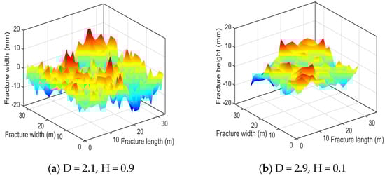
Figure 2.
The roughness of the fracture under different fractal dimensions.
Many scholars have studied fluid dynamics in pipeline flow [27], combined with existing fractal models of relative roughness, and the morphology of fractures, using laminar flow of non-Newtonian fluids with low Reynolds numbers in cylindrical capillary models [28]. The model is used to derive the relationship between the relative roughness and the tortuosity in the cylindrical channel to characterize the roughness [29].
Figure 3a is a schematic diagram of the rough cylindrical capillary model. Figure 3b is a schematic diagram of the rough cross-section profile and the rough element distribution of the cylinder. Each bulge in the figure is a cross-sectional profile of the rough element. The radius (capillary diameter) of the cylindrical channel model is . Based on the above model, the following can be calculated:

Figure 3.
Capillary (a) rough cylindrical capillary model, and (b) rough cylindrical cross-section profile and rough element distribution.
The relative roughness of the fracture is as follows:
The effective radius of the rough element is as follows:
The total volume of fractures is as follows:
The total volume of capillary inner surface roughness element is as follows:
The fracture tortuosity is as follows:
Bring Equations (2)–(5) into Equation (1), as follows:
where is the relative roughness of fractures; is the effective radius of the rough element, mm; is the effective radius of drilling fluid circulation, mm; is the inner radius of the fracture, mm; is the total volume of the capillary, mm3; is the total volume of the roughness element on the inner surface of the tube, mm3; is the fracture extension length, m; is the actual length in the fracture, m; is the tortuosity of fracture.
It can be seen from this formula that the relative roughness of fractures is related to the tortuosity and volume of fractures. The model does not contain any empirical parameters, and each parameter has a clear physical meaning.
Equation (6) is deformed to obtain the following:
At present, some scholars have used the fractal method [13,14] to represent the fracture roughness in the leakage model and have used the fracture tortuosity [15] to characterize the fracture roughness—see Equation (8)—which can also express the influence of fracture roughness on fracture mechanical opening, as follows:
where is the mechanics opening of fracture, ; is the hydraulic aperture of fracture, .
Since the opening of fracture mechanics is directly related to the total volume and diameter in the fracture, Equation (7) can be reasonably simplified to Equation (8).
Compared with the linear deformation formula, the fracture index deformation formula can better describe the dynamic change behavior of fracture width as follows:
where is the static width of fracture, ; is the fracture width index deformation coefficient, ; is the seam pressure, ; is the formation pore pressure, .
3. Drilling Fluid Leakage Model
For fractured complex formations, the filtrate leakage of drilling fluid on the fracture surface is much smaller than the leakage of drilling fluid inside the fracture when focusing on the leakage inside the fracture. In order to better simulate the leakage of drilling fluid, a radial leakage model for H-B drilling fluid was established. Various influencing factors, such as drilling fluid consistency coefficient, drilling fluid dynamic shear force, fracture width, fracture roughness (curvature, fracture index deformation coefficient), pressure difference, and the radial extension length of drilling fluid, are studied to improve the radial model.
Assumptions made for the model are as follows:
- 1
- Filtrate leakage on the fracture surface is negligible;
- 2
- The initial pressure of the fracture is the formation pressure;
- 3
- The fracture extends infinitely in the radial direction;
- 4
- The fluid flow inside the fracture is laminar flow;
- 5
- The compressibility of drilling fluid is not considered;
- 6
- The width of the fracture is much smaller than the height and length;
- 7
- The drilling fluid leakage velocity in the height direction of the fracture is relatively small compared to the leakage velocity in the length direction of the fracture.
3.1. Mathematical Model
As shown in Figure 4, it is assumed that the fracture extends infinitely into the formation; the longitudinal leakage velocity (Z axis) of drilling fluid in the fracture is very small compared with the transverse leakage velocity (r direction), which can be ignored.
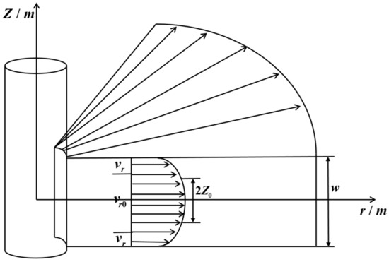
Figure 4.
Radial flow model of drilling fluid in the fracture of the wellbore.
At present, three models of drilling fluid rheology are described (Figure 5). Since the initial dynamic shear force is one of the rheological properties of drilling fluid, the drilling fluid will flow only when the external force reaches or exceeds this initial value. The Bingham model is the initial value, which is generally much higher than the actual drilling fluid limit dynamic shear force, while in the power-law model rheological curve through the origin, the initial shear force is zero, so the two traditional models cannot better reflect this characteristic. Considering that drilling fluids are non-Newtonian fluids [19], the rheological model of drilling fluid is the H-B model.

Figure 5.
Fluids with different rheological modes.
3.2. Drilling Fluid Leakage Model
The drilling fluid is a viscous fluid, and the flow law conforms to the NS equation.
- 1
- The constitutive equation of the H-B flow pattern is as follows:
- 2
- The continuity equation along the radial direction of the wellhead around the wellbore is as follows:
- 3
- The momentum conservation equation in the radial direction is as follows:
- 4
- The momentum equation can be substituted into the N-S equation to obtain the following:
Combining the fluid constitutive equation and integrating, the average velocity is obtained by omitting the high-order term after Taylor expansion, as follows:
Bring Equation (7) into the continuity equation to obtain the following:
3.3. Model Solving
The model equation is a non-steady-state second-order equation with fraction order, which is difficult to solve. Although the explicit method is easier to solve, it is necessary to consider the step ratio, and different step ratios will lead to different errors with the increase in the number of calculation layers, which may also make the results diverge. Therefore, the implicit difference method [30] is used to solve the problem, and the result is absolutely convergent. The flow pattern index n = 1 is used for simplified calculation. For this equation, the following equation is obtained by difference:
Using the approximate method, the first item in the right bracket is expanded as follows:
The second expansion is:
Therefore, the equation can be approximately written as follows:
Among them are the following:
The backward Euler scheme with absolute stability (the calculation result must be convergent and credible, not limited by space step and time step) is used to calculate the following:
The equation is expanded as follows:
Multiply both sides of the above equation by to obtain the following:
This difference equation is a tridiagonal equation, written in the form of a matrix as follows:
3.4. Model Boundary Conditions
The simulation uses the following boundary conditions:
where is the wellbore pressure, ; is the borehole radius, ; is the radius of the fracture extending to the fracture tip, ; is the time when the fracture extends to the fracture tip, .
4. Drilling Fluid Leakage Pattern
Table 1 shows the initial data for analyzing the factors of each parameter in the mathematical model for the fracture-based leakage of H-B drilling fluids.

Table 1.
Basic parameters of numerical simulation of leakage model.
4.1. Consistency Coefficient of Drilling Fluid
By controlling the influence of other parameters, the consistency coefficient of drilling fluid is taken as 0.2 , 0.4 , 0.6 , and 0.8 , and the leakage law of drilling fluid under the consistency coefficient of drilling fluid at different times is simulated by numerical analysis; the results are shown in Figure 6:
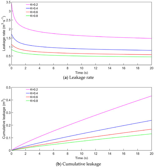
Figure 6.
Effect of drilling fluid viscosity coefficient on leakage.
As shown in Figure 6, it can be observed that the consistency coefficient of the drilling fluid gradually decreases with increasing time. The higher the consistency coefficient, the lower the rate and cumulative amount of fluid leakage. When time changes within a certain range, the trend of the fluid leakage rate curve becomes slower, and the slope of the cumulative fluid leakage curve also changes slowly, resulting in the maximum cumulative fluid leakage. The viscosity coefficient of the drilling fluid affects its flowability in the fracture, and the greater the additional friction, the smaller the fluid leakage rate and the amount of fluid leakage.
4.2. Dynamic Shear Force of Drilling Fluid
Simulate the leak characteristic curves (Figure 7) of dynamic shear force at 10 Pa, 15 Pa, 20 Pa, and 25 Pa, respectively, while controlling the influence of other parameters.
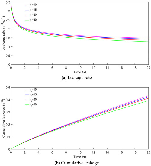
Figure 7.
Effect of drilling fluid dynamic shear force on leakage.
As shown in Figure 7a,b, the larger the dynamic shear force, the smaller the fluid leakage rate, and the lower the cumulative fluid leakage. This indicates that the presence of dynamic shear force to some extent affects the fluid leakage rate in the fracture, and adjusting this factor can effectively reduce the cumulative fluid leakage. However, the effect of dynamic shear force on fluid flow is much smaller than that of pressure gradient in the wellbore at the given depth level. Therefore, in the figure, there is no significant difference in the fluid leakage rates among several different dynamic shear forces, which also have little impact on the cumulative fluid leakage.
4.3. Initial Aperture of Fracture
Simulate the leak characteristic curves while controlling the influence of other parameters, with initial fracture widths of 1.0 mm, 1.5 mm, 2.0 mm, and 3.0 mm, respectively; the results are shown in Figure 8.
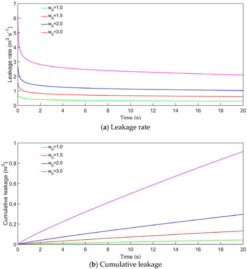
Figure 8.
Effect of initial fracture opening on leakage.
Based on the classification of the solid phase of the drilling fluid, the solid phase of the drilling fluid is at the micro level and can effectively pass through the assumed width of the fracture. As shown in Figure 8, the larger the initial fracture width, the faster the instantaneous fluid leakage rate, and the larger the cumulative fluid leakage. At the initial stage of fluid leakage, the fluid leakage rate reaches a peak value, but with the increase in fluid leakage time, the fluid leakage rate begins to flatten. This is because the infiltration rate of the drilling fluid in the fracture is much larger than that of the formation. However, due to the particle size, there are microfractures in the fracture that can be blocked by solid phase particles, which restricts the flow channel of the fracture.
From Equation (8), it can be seen that in the case of constant pressure conditions in the fracture, the larger the initial fracture opening, the larger the fracture opening that provides a good fluid leakage channel for the drilling fluid and exacerbates the fluid leakage.
4.4. Fracture Index Deformation Coefficient
Simulate the leak characteristic curves while controlling the influence of other parameters, with fracture index deformation coefficients of 8.6 × 10⁻⁸, 1.29 × 10⁻⁷, 1.72 × 10⁻⁷, and 2.58 × 10⁻⁷, respectively; the results are shown in Figure 9.
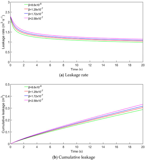
Figure 9.
Effect of fracture index deformation coefficient on leakage.
As shown in Figure 9, as the deformation coefficient of the fracture index increases, the fluid leakage rate and the cumulative fluid leakage amount within the fracture increase, and the ultimate fluid leakage rate value is also larger than that of other parameter values. With the gradual decrease in the deformation coefficient, the fluid leakage rate curve is similar to the cumulative fluid leakage curve. The smaller the deformation coefficient of the fracture index, the smaller the change in the fracture width with the change in the fluid pressure in the fracture, and the less likely the fracture is to deform. However, with the increase in the deformation coefficient, the increase in fluid pressure inside the fracture can be moderated by the deformation index. Therefore, the larger the deformation coefficient, the easier the fracture shape changes, and the greater the change in the width.
4.5. Fracture Tortuosity
Simulate the leak characteristic curves while controlling the influence of other parameters, with fracture tortuosities of 1.0, 1.5, 2.0, and 3.0, respectively; the results are shown in Figure 10.
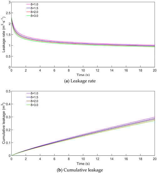
Figure 10.
Effect of fracture tortuosity on leakage.
Figure 10 shows that the smaller the curvature of the fracture, the larger the fluid leakage rate and the cumulative fluid leakage amount. With the prolongation of time, the fluid leakage rate of the drilling fluid gradually tends to be stable within the fracture. Under the condition that the curvature of the fracture is two times different, there is no significant difference in the characteristic curve of fluid leakage, indicating that the degree of influence of the fracture curvature on fluid leakage is small. Since the curvature refers to the ratio of the total length of the fracture to the horizontal length of the fracture, the smaller the curvature value, the smoother the fracture, the lower the flow resistance of the fluid, and the larger the fluid leakage rate. Although the impact of the fracture curvature on the fluid leakage rate is small, due to the special nature of the fracture, it cannot be completely ignored.
4.6. Pressure Differential
Maintain initial fracture pressure at 20 MPa and simulate the leak characteristic curves while controlling the influence of other parameters, with wellbore fluid column pressures of 30 MPa, 35 MPa, 40 MPa, and 45 MPa, respectively; the results are shown in Figure 11.
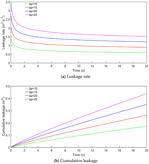
Figure 11.
Effect of pressure difference on leakage.
As shown in Figure 11, when the bottom hole pressure difference changes from 10 MPa to 25 MPa, the fluid leakage rate of the drilling fluid increases significantly, and the cumulative fluid leakage amount also increases, showing a trend of multiplicative growth. At the initial moment of fluid leakage, the fluid leakage rate of the drilling fluid reaches the peak value, and there is a significant difference between the final stable state. The main reason for the fluid leakage of the drilling fluid is due to the pressure difference between the static column pressure and the formation pressure. The larger the bottom hole pressure difference, the more serious the fluid leakage situation and the greater the risk. With the increase in the pressure difference and under the hydraulic effect, the length and width of the fracture will increase, the fluid flow channel of the drilling fluid will be larger, and the fluid leakage will be more serious.
4.7. Radial Extension Length
With other parameters set constant, simulate the leak feature curves while controlling the radial extension length, the depth of invasion of the drilling fluid, at 0 m, 5 m, 10 m, and 15 m, respectively; the results are shown in Figure 12.
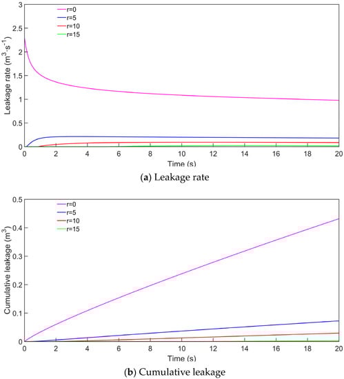
Figure 12.
Effect of radial extension length on leakage.
As shown in Figure 12, as the depth of drilling fluid intrusion increases, the rate of drilling fluid leakage gradually decreases, and the trend of cumulative leakage gradually slows down. On the wall at the point where the leakage is 0 m, the characteristics of drill−ing fluid leakage are obvious. At the beginning of the leakage time, there is a significant downward trend in leakage, and, as the time increases, the radial extension length in−creases, the leakage rate and peak become smaller, and the cumulative leakage amount progresses slowly. This is because the surface of the fracture is rough, causing additional resistance to the fluid flow and resulting in the leakage of drilling fluid. When the radial extension length reaches a certain point, the fracture tip pressure tends to be the formation pressure, the bottom hole pressure difference becomes 0, and the leakage stops. Figure 12b can better characterize the relationship between the extension length and the cumulative leakage amount. At the beginning of the leakage, the leakage has not yet extended to the point of 15 m, and the cumulative leakage amount is 0 at this time. With the leakage inside the fracture, the cumulative leakage amount begins to change but changes slowly. Due to the high pressure at the tip of the fracture, when the fluid reaches the tip, it cannot support a large pressure, causing the formation to be compacted, and no pressure difference exists. At this time, the pressure at the tip is the formation pressure.
5. Discussion
From Figure 6, Figure 7, Figure 8, Figure 9, Figure 10, Figure 11 and Figure 12, it can be seen that the most significant factors affecting the fracture are the pressure difference and fracture width (Figure 8 and Figure 11) when the initial leakage rate and the final cumulative leakage are both high. In the petroleum industry, not only is drilling fluid leakage a problem, but so too is fracturing fluid leakage. Although drilling fluid leakage causes a relatively small decrease in pressure, fracturing fluid causes a significant pressure drop. Fracturing fluid itself accumulates at high pressure to generate fractures in the formation, which is different from drilling fluid, but they both belong to the fluids group. The pressure leakage caused by a leakage may completely block the formation, resulting in no fracture creation and closure of the original oil flow channel in the formation. At this point, an efficient solution for oil recovery becomes a problem. To reduce such leakages, studying drilling fluid leakage can provide valuable references for fracturing fluid leakage, as their viscosity is the most significant difference between them.
In the future, research can focus on simplifying different flow index models to provide better solutions to fluid leakage problems in the petroleum industry.
6. Conclusions
This article selects the high-precision computational H-B flow type drilling fluid and establishes a non-steady-state radial leakage model, analyzing the influence of various parameters on leakage characteristics. The following conclusions are obtained:
(1) For radial leakage models in geological formations with fractures, we find that roughness has an important impact on the fracture leakage model.
(2) Consistency coefficient, tortuosity, and dynamic shear force of the drilling fluid is negatively correlated with the leakage rate and cumulative leakage; the fracture index de-formation coefficient, pressure difference and initial fracture width are positively correlated with the leakage rate and cumulative leakage. Controlling the degree of leakage mainly involves controlling the pressure difference and fracture opening parameters.
(3) As time increases, the depth of drilling fluid invasion increases, and the stress on the fracture gradually increases, causing the leakage rate to gradually decrease and eventually become zero; the change in cumulative leakage quantity weakens and eventually becomes constant.
Author Contributions
Conceptualization, Z.X. and S.B.; methodology, S.B.; software, M.H.; validation, T.W. and H.W.; formal analysis, Z.X.; investigation, S.B.; writing—original draft preparation, Z.X.; writing—review and editing, L.Z.; visualization, H.J. and H.Z.; supervision, L.Z.; funding acquisition, H.W. All authors have read and agreed to the published version of the manuscript.
Funding
This research was funded by the 13th Five-Year National Science and Technology Major Project, grant number 2016ZX05061-009.
Data Availability Statement
Data is unavailable due to privacy.
Acknowledgments
The author thanks Zhu of Yangtze University for his valuable research ideas and writing help.
Conflicts of Interest
The authors declare no conflict of interest.
References
- Zhao, W.B. Study on the mechanism of induced fracture leakage and the countermeasures of preventing and plugging in Liujiagou Formation of Hangjinqi. In Proceedings of the 2018 National Natural Gas Academic Annual Conference (04 Engineering Technology), Fuzhou, China, 14 November 2018; pp. 78–83. [Google Scholar]
- Tan, Z.J.; Hu, Y.; Yuan, Y.D.; Cao, J.; Zhang, Q.Q.; Yang, Z.X. Study on the mechanism of lost circulation in fractured formations in Bohai Sea-Taking Bozhong 34-9 oilfield as an example. China Pet. Explor. 2021, 26, 127–136. [Google Scholar]
- Cui, G.J.; Zhu, G.W.; Su, J.; Gao, K.C. Study on wellbore stability of Bohai deep well. Petrochem. Technol. 2021, 28, 93–94+100. [Google Scholar]
- He, R.b.; Xu, J.; Wang, H.W. High-efficiency plugging technology for fault fracture leakage in Bo hai Oilfield. J. Yangtze Univ. (Sci. Ed.) 2015, 12, 38–42. [Google Scholar]
- Chen, X.H.; Qiu, Z.S.; Yang, P.; Guo, B.Y.; Wang, B.T.; Wang, X.D. Dynamic simulation of fracture leakage process based on ABAQUS. Drill. Fluid Complet. Fluid 2019, 36, 15–19. [Google Scholar]
- Gaurina-Međimurec, N.; Pašić, B.; Mijić, P.; Medved, I. Drilling Fluid and Cement Slurry Design for Naturally Fractured Reservoirs. Appl. Sci. 2021, 11, 767. [Google Scholar] [CrossRef]
- Huang, F.S. Numerical Simulation of Drilling and Completion Fluid Leakage in Natural Fracture Network System. Master’s Thesis, Southwest Petroleum University, Chengdu, China, 2014. [Google Scholar]
- Lietard, O.; Unwin, T.; Guillot, D.; Hodder, M. Fracture Width LWD and Drilling Mud/LCM Selection Guidelines in Naturally Fractured Reservoirs. In Proceedings of the European Petroleum Conference, Milan, Italy, 22–24 October 1996. [Google Scholar]
- Lietard, O.; Unwin, T.; Guillo, D.J.; Hodder, M.H. Fracture Width Logging While Drilling and Drilling Mud/Loss-Circulation-Material Selection Guidelines in Naturally Fractured Reservoirs. SPE Drill. Complet. 1999, 14, 168–177. [Google Scholar] [CrossRef]
- Ozdemirtas, M.; Babadagli, T.; Kuru, E. Effects of fractal fracture surface roughness on borehole ballooning. Vadose Zone J. 2009, 8, 250–257. [Google Scholar] [CrossRef]
- Ozdemirtas, M.; Kuru, E.; Babadagli, T. Experimental investigation of borehole ballooning due to flow of non-Newtonian fluids into fractured rocks. Int. J. Rock Mech. Min. Sci. 2010, 47, 1200–1206. [Google Scholar] [CrossRef]
- Shahri, M.P.; Mehrabi, M. A new approach in modeling of fracture ballooning in naturally fractured reservoirs. In Proceedings of the SPE Kuwait International Petroleum Conference and Exhibition, Kuwait City, Kuwait, 10–12 December 2012. [Google Scholar]
- Li, D.Q.; Kang, Y.L.; Liu, X.S.; Chen, C.W.; Si, N. Research progress on dynamic model of drilling fluid loss in fractured formations. Oil Drill. Technol. 2013, 41, 42–47. [Google Scholar]
- Li, S.; Kang, Y.L.; Li, D.Q.; Tang, L.; Yang, J.; Liu, X.F. Lost circulation model and experimental simulation of H-B flow pattern drilling fluid in fractured formation. Pet. Drill. Process 2015, 37, 57–62. [Google Scholar]
- Li, D.Q. Study on Drilling Fluid Leakage Kinetics in Fractured Formations. Ph.D. Thesis, Southwest Petroleum University, Chengdu, China, 2012. [Google Scholar]
- Jia, L.C.; Chen, M.; Hou, B.; Sun, Z.; Jin, Y. Drilling fluid loss model and law in fractured formations. Pet. Explor. Dev. 2014, 41, 95–101. [Google Scholar] [CrossRef]
- Song, T.; Zhao, X.Y. Research and application of leakage model in fractured formation, science and technology and engineering. J. Mater. Chem. A 2013, 13, 9191–9195. [Google Scholar]
- Lavrov, A. Numerical modeling of steady-state flow of a non-Newtonian power-law fluid in a rough-walled fracture. Comput. Geotech. 2013, 50, 101–109. [Google Scholar] [CrossRef]
- Shi, X.Y. Fracture Opening, Propagation and Leakage in Carbonate Formation. Master’s Thesis, China University of Petroleum, Qingdao, China, 2017. [Google Scholar]
- Zhai, X.P.; Chen, H.; Lou, Y.S.; Wu, H.M. Prediction and control model of shale induced fracture leakage pressure. J. Pet. Sci. Eng. 2021, 198, 108186. [Google Scholar] [CrossRef]
- Jing, C.; Duan, Q.; Han, G.; Nie, J.; Li, L.; Ge, M. Quantitative Interpretation Model of Inter well Tracer for Fracture-Cavity Reservoir Based on Fracture-Cavity Configuration. Processes 2023, 11, 964. [Google Scholar] [CrossRef]
- Hu, R.; Wang, C.; Zhang, M.; Zhang, Y.; Zhao, J. The Study of Multi-Scale Specific Surface Area in Shale Rock with Fracture-Micropore-Nanopore. Processes 2023, 11, 1015. [Google Scholar] [CrossRef]
- Wu, H.Y.; Zhu, L.F. Application of imaging and nuclear magnetic resonance logging in the evaluation of Chengbei fractured reservoir. Pet. Nat. Gas Geol. 2002, 23, 45–48. [Google Scholar] [CrossRef]
- Mandelbrot, B.B. The Fractal Geometry of Nature; W. H. Freeman and Company: San Francisco, CA, USA, 1982. [Google Scholar]
- Brown, S.R. Fluid flow through rock joints: The effect of surface roughness. J. Geophys. Res. 1987, 92, 1337–1348. [Google Scholar] [CrossRef]
- Bi, S.B.; Zhang, Y.; Zhou, Z.; Lou, Y.S.; Zhou, R.; Zhang, X.M. Study on the Model and Law for Radial Leakage of Drilling Fluid in Fractured Formations. ACS Omega 2022, 7, 39840–39847. [Google Scholar] [CrossRef]
- Mustafa, T. Eyring–Powell fluid flow through a circular pipe and heat transfer: Full solutions. Int. J. Numer. Methods Heat Fluid Flow. 2020, 30, 4765–4774. [Google Scholar] [CrossRef]
- Pinho, F.T.; Whitelaw, J.H. Flow of non-newtonian fluids in a pipe. J. Non-Newton. Fluid Mech. 1990, 34, 129–144. [Google Scholar] [CrossRef]
- Qu, G.Z. Description of Rough Fracture Structure and Its Seepage Law. Ph.D. Thesis, China University of Petroleum, Qingdao, China, 2016. [Google Scholar]
- Sun, Z.Z. Numerical Solution of Partial Differential Equations; Science Press: Beijing, China, 2012. [Google Scholar]
Disclaimer/Publisher’s Note: The statements, opinions and data contained in all publications are solely those of the individual author(s) and contributor(s) and not of MDPI and/or the editor(s). MDPI and/or the editor(s) disclaim responsibility for any injury to people or property resulting from any ideas, methods, instructions or products referred to in the content. |
© 2023 by the authors. Licensee MDPI, Basel, Switzerland. This article is an open access article distributed under the terms and conditions of the Creative Commons Attribution (CC BY) license (https://creativecommons.org/licenses/by/4.0/).