Robustness Prediction in Dynamic Production Processes—A New Surrogate Measure Based on Regression Machine Learning

Abstract

This feasibility study utilized regression models to predict makespan robustness in dynamic production processes with uncertain processing times. Previous methods for robustness determination were computationally intensive (Monte Carlo experiments) or inaccurate (surrogate measures). However, calculating robustness efficiently is crucial for field-synchronous scheduling techniques. Regression models with multiple input features considering uncertain processing times on the critical path outperform traditional surrogate measures. Well-trained regression models internalize the behavior of a dynamic simulation and can quickly predict accurate robustness (correlation: $r>0.98$). The proposed method was successfully applied to a permutation flow shop scheduling problem, balancing makespan and robustness. Integrating regression models into a metaheuristic model, schedules could be generated that have a similar quality to using Monte Carlo experiments. These results suggest that employing machine learning techniques for robustness prediction could be a promising and efficient alternative to traditional approaches. This work is an addition to our previous extensive study about creating robust stable schedules based on deep reinforcement learning and is part of the applied research project, Predictive Scheduling.

1. Introduction

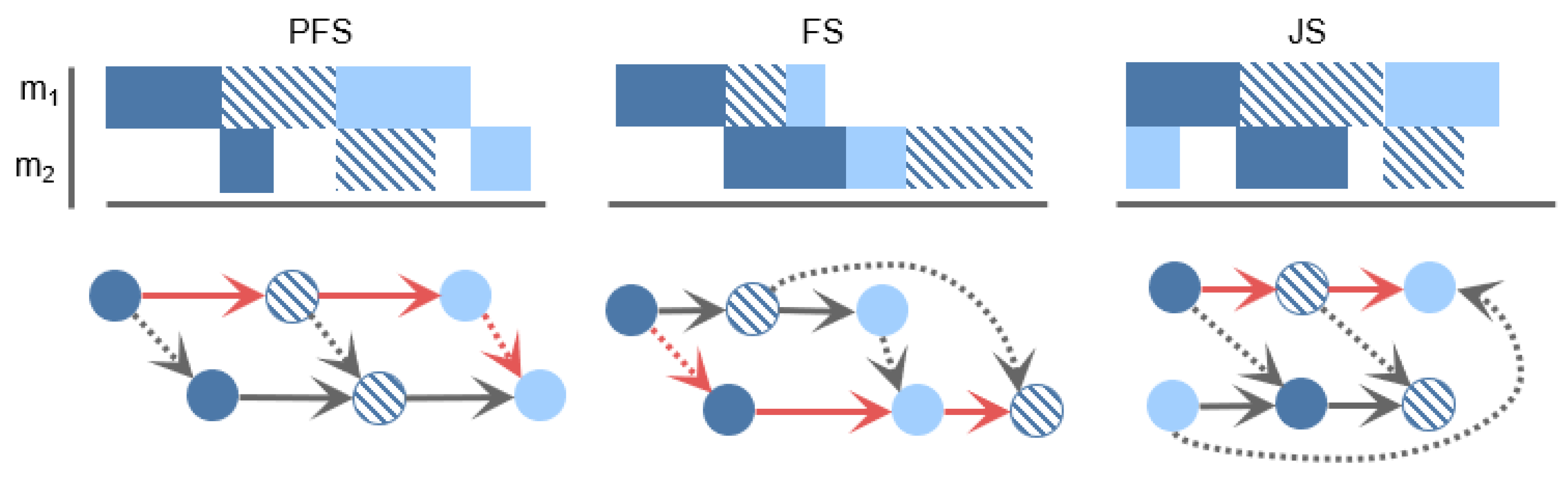
1.1. Production Environments and Schedule Representations

In order to highlight the relevance of an efficient robustness estimation, production environments and the representability of production schedules must be introduced. Production schedules can be generated by mathematical methods for sequencing activities by assigning them to limited resources in order to optimize an objective function [1]. To depict different forms of manufacturing with specific constraints, a variety of optimization models have been developed. Permutation flow shops (PFSs), which can often be found in the industry, are suitable as an introductory example. According to Rossi et al. [2], the following constraints apply in traditional PFSs regardless of uncertainties:

• Every production job has m operations (activities), each to be processed on a different machine (resource);
• Within each job, the machines must be visited in a sequential order $1,\dots ,m$;
• Operations of a job can only start when any previous operations of the job have been completed;
• Each machine can only process one operation at a time;
• The job order is equal for all machines (jobs cannot overtake each other in the line);
• All operations must be processed exactly once and non-preemptively.

Common deterministic objectives minimize the makespan ($min{C}_{max}$), flow time or total tardiness of jobs. Although the model is comparatively easy to formulate and has only one decision variable (order of jobs on the first machine), it is a non-deterministic polynomial-time (NP) hard problem [2].

Other well-known production environments are the flow shop (FS), and job shop (JS) as well as their flexible forms. The FS problem is a generalization of the PFS problem without considering constraint 5. Accordingly, jobs in the production line can overtake each other. The JS is another generalization of the FS without considering constraint 2. As a result, the jobs can be based on different material flows with different machine orders. In flexible environments, a machine must be selected from a set of alternatives for each operation. This makes the problems even more difficult to solve, since a resource allocation decision must also be made in addition to the sequencing decision  [1].

Regardless of specific constraints and decision variables, a feasible solution to these problems can be represented as a directed acyclic solution graph (DASG) $G(O,\mathsf{\Psi })$ [3], where O is the set of scheduled operations, and $\mathsf{\Psi }$ is the set of directed predecessor relationships between the operations. For traditional production scheduling models with one resource type and $m\ge 2$ machines, every operation vertex in the DASG has $\mathsf{\Phi }\in \{0,1,2\}$ outgoing and incoming edges. Figure 1 shows different exemplary solutions to PFS, FS and JS problems with three jobs and two machines. In addition to the DASG, a Gantt chart is presented at the top to visualize the assigned operations on the timeline. The red arrows highlight the critical path of the schedule. Dashed arrows represent job successors, and solid arrows represent machine successors.

1.2. Robustness Measures

Since many real-world production processes are influenced by uncertainties, there has been a substantial amount of research on scheduling in dynamic environments that takes into account factors such as uncertain processing times (UPTs) or dynamic events such as machine failures. In contrast to reactive rescheduling, robust (syn. proactive, predictive) scheduling plays a crucial role in anticipating uncertainties in advance. The aim is to create a robust schedule (RS) in such a way that occurring events change its baseline structure as minimally as possible  [4,5,6,7].

Consequently, a robust scheduling problem is an extension of its deterministic counterpart considering uncertainties and further objectives for robustness optimization [8]. Generally formulated, a baseline objective ($minZ$) is balanced with a robustness objective ($minR$). In addition, a number of constraints ${\Theta }_1,\dots ,{\Theta }_{\eta }$ with stochastic parameters are considered:

$$\begin{array}{cc}\hfill & minZ\hfill \\ & minR\hfill \\ & \mathrm{s}.\mathrm{t}.\hfill \\ & {\Theta }_1,\dots ,{\Theta }_{\eta }\hfill \end{array}$$

Regarding R, prior studies such as [4,9] established a definition for robustness: A schedule is robust when the performance of a realized robust schedule (RS*) deviates as minimally as possible from the performance of its baseline RS. The performance deviation refers to a schedule metric Z (e.g., $C_{max}$) before and after realization:

$$\begin{array}{c}\hfill R=R{S}_Z-R{S}_Z^{\ast }\end{array}$$

In order to obtain a reliable result, Monte Carlo experiments (MCEs) are required to determine uncertainty effects in complex stochastic settings. Alternatively, surrogate measures (SMs) can be used to quickly but inaccurately estimate R (see Section 1.3). In connection with positive robustness values ($R>0\iff R{S}_Z>R{S}_Z^{*}$), the RS was planned too conservatively. Otherwise, if $R<0\iff R{S}_Z<R{S}_Z^{*}$, the RS is too optimistic. Figure 2 visualizes this effect: After realization of a schedule, there is a deviation between the planned and actual makespan ($R{S}_{C_{max}}<R{S}_{C_{max}}^{*}$). Consequently, the RS was planned too optimistically. The figure also shows machine idle times $x_1,\dots ,x_3$, where an operation is not assigned to the resource. $x_2$ is a slack time between two operations that can be used to extend the preceding operation without affecting the overall structure of the schedule.

In the context of robust scheduling, several authors consider stability S as a second measure. According to most authors, a schedule is stable when the realized operations $o\in R{S}_O^{*}$ are terminated as defined a priori [9]. Thus, S can be calculated by the sum of absolute deviations of operation completion times $o_e$:

$$\begin{array}{c}\hfill S=\sum _{i=1}^{|R{S}_O^{*}|}|{\left(R{S}_{O_i}\right)}_e-{\left(R{S}_{O_i}^{*}\right)}_e|\end{array}$$

Robustness R and stability S have been identified as conflicting measures [9,10,11,12]. Moreover, both measures are in a triangular conflict with several baseline objectives [10,12]. For this reason, it is recommended that robust scheduling methods balance these three dimensions. Complementary to robustness measures, another part of the literature took focus on fuzzy numbers, where different model parameters such as processing times or due dates are represented as fuzzy intervals [13,14]. The practical advantage of using fuzzy numbers is the easy calculability of operation completion times [3] or waiting times [15]. However, the calculation of robustness is likely not trivial in the context of more complex uncertainty models and cannot be performed analytically [16]. This suggests that the robust scheduling literature beyond fuzzy intervals mainly utilized SMs or MCEs.

1.3. Robust Scheduling Techniques

As this work is supplementary to our prior research, we direct readers to the section “Literature Review” presented in [17], which provides an overview of relevant studies in the field of robust scheduling. The studies have been classified based on the following four dimensions:  

• Scheduling stage: (A) RS generation in a second stage based on a given DASG. (B) Aggregated with baseline objective optimization.
• Optimization technique: (A) Adding buffer times to critical operations. (B) Creating neighbor solutions, e.g., by swapping operations.
• Evaluation technique: (A) Obtaining robustness by MCE. (B) Estimating robustness by SMs.
• Robustness objective: (A) Standalone robustness [R]. (B) Robustness and stability [$R,S$]. (C) Robustness, stability and baseline objective [$R,S,Z$].

This study pays special attention to the third dimension, the evaluation technique. Either R can be estimated by using SMs (see [5,8,16]) or by performing MCEs (see [4,10,11,18]). On the one hand, MCEs require a lot of computational time but generate reliable results [16]. On the other hand, SMs, which are arithmetic measures to approximate R or S without performing MCEs, can be calculated quickly but show an insufficient accuracy [8]. Traditional SMs are total or free slack time per operation, number of critical path operations per machine and average makespan per neighbor RS [19]. Zahid et al. [20] provided a comprehensive survey of surrogate measures utilized both in production and project scheduling. Their objective was to investigate various parameters that can aid the assessment of robustness in the context of tardiness in project scheduling. Their results underline the importance of total slack. More sophisticated SMs are presented in [8,16,21]. Xiao et al. [8] presented two new surrogate measures that both consider the estimated robustness degradation of the critical path as well as of the non-critical path. The authors highlighted the importance of the inspection of the non-critical path, since other studies such as [22] only considered operations on the critical path of a schedule. In a follow-up study [16], the authors analyzed how the expected delay in the schedule realization is propagated downstream the schedule. Both studies share a common set of limitations. Firstly, they necessitate a parameter set by a decision maker. Secondly, the proposed surrogate measures are exclusively applicable for normally distributed processing times. In each study, the authors recommended further research for different distribution types. Yang et al. [21] criticized the fact that many SMs under-utilize the available information contained in a schedule. Thus, the authors utilized a single-hidden layer feedforward network with an extreme learning algorithm to predict the robustness. Three types of information are integrated in the prediction, namely probability of machine breakdown, workload and location of total slack. The proposed method eliminates the need for manual weighting of the three factors. The authors recommended extending this approach to other types of uncertainties, such as uncertain processing times. To the best of our knowledge, this is the only approach that utilizes machine learning (ML) for robustness estimation. In contrast to these highly specific surrogate measures designed for an individual class of problems, Himmiche et al. [23] proposed a modeling framework based on stochastic timed automata that enables robustness evaluation based on evaluation and model-checking techniques. The primary benefit of this approach lies in its versatility, as it can be easily adapted to different types of workshops and different types of uncertainties. Conversely, a significant shortcoming is the computation time, which dramatically increases the the size of the workshop.

1.4. Motivation and Contribution of This Work

The study is motivated by lack methods to predict robustness measures, which are efficient and accurate at the same time. According to Section 1.3, robust scheduling methods utilize computationally intensive MCEs to obtain these measures, or SMs, which are either imprecise due to under-utilization of available information or are highly specific and thus not applicable to a wide range of problems. This leads to decisive disadvantages and shortcomings in field-synchronous scheduling methods. Thus, it should be investigated how the advantages of accuracy and computational efficiency can be combined. The contribution of this work is a method that merges the beneficial attributes of the methods outlined in Section 1.3. It combines

• the analysis of disturbance propagation throughout the schedule [16];
• the utilization of different types of information in combination with ML [21];
• and the versatility presented in [23].

The approach utilizes regression models (RMs) to predict the makespan robustness ($R=R{S}_{C_{max}}-R{S}_{C_{max}}^{*}$) based on generic DASGs with gamma distributed UPTs. Operations, machines, noisy operations end times, idle and slack times are considered as a priori input features for the RMs. In Section 2, the scope of the method is narrowed down. Moreover, hypotheses for validating the method are presented. Subsequently, details of the RMs, the training data and the implementation are described. According to the hypotheses, the results are presented and discussed in Section 3. It could be shown that RMs can predict very accurate robustness scores in a very short computing time and without computationally intensive MCEs.

2. Method

In this chapter, we first present the scope and utility of the proposed method and formulate hypotheses for verifying its contribution. Subsequently, we describe mathematical modeling, implementation specifics, and training data related to the RMs.

2.1. Scope and Utility

In general, the prediction method is independent of the specific baseline problem, since it is already based on the DASG representation of a generated schedule. It can therefore be used for job shops and flow shops with $m>1$ machines regardless of specific constraints and baseline objectives. Due to the universal calculation of uncertainties and their effect on the critical path (see Section 2.4), the method can also be applied to other types of distributions. However, further uncertainties such as dynamic release times or due dates are not taken into account in this proof-of-concept study.

To illustrate the utility and applicability of the method, Algorithm 1 provides a simplified robust scheduling trajectory search. It is an abstract algorithm to show the basic procedure of many current heuristics to optimize a baseline objective and/or robustness measures. Here, a search method with $\overline{n}$ iterations is conducted, which successively generates neighborhood solutions of a schedule to identify a good local optima considering stochastic and deterministic objectives. When utilizing MCEs in the $EVAL$ function to obtain the robustness, a large number of simulations is required in complex environments (see Section 2.5). It is even conceivable that the number of MCEs $\overline{m}$ is larger than the number of search iterations $\overline{n}$. This leads to a complexity of $O\left(\overline{n}\overline{m}\right)⪆O\left({\overline{n}}^2\right)$, which can be a crucial bottleneck in reactive real-time environments with extensive simulations. Integrating a RM into the $EVAL$ function, the number of simulations can be substituted with a singular prediction, which corresponds to a reduced complexity of $O\left(\overline{n}\right)$. In this way, the same complexity prevails, as is the case with SMs.

Algorithm 1 Exemplary local search robust scheduling heuristic (simplified pseudocode)
1: $R{S}_1\leftarrow CIS\left(O\right)$	▹ Create initial schedule based for a set of operations O (output: DASG)
2: $R{S}_1^{*}\leftarrow EVAL\left(R{S}_1\right)$	▹ Evaluate the initial schedule considering uncertainties
3: for $i\leftarrow 1,i\le \overline{n},i\leftarrow i+1$ do	▹ Conduct a local search for $\overline{n}$ iterations
4:       $R{S}_2\leftarrow CNS\left(R{S}_1\right)$	▹ Create neighbor solution, e.g., by changing the operation order
5:       $R{S}_2^{*}\leftarrow EVAL\left(R{S}_2\right)$	▹ Evaluate the neighbor
6:        if $FIT\left(R{S}_2^{*}\right)>FIT\left(R{S}_1^{*}\right)$  then
7:              $R{S}_1\leftarrow R{S}_2$	▹ Replace the current schedule if the neighbor has a better fitness
8:        end if
9: end for
10: return $R{S}_1^{*}$

2.2. Hypotheses and Statistical Measures

In order to concretize the contribution of this study (see Section 1.4), the following hypotheses are formulated and tested in the experiments:

H1. 

If EPTs are utilized to create an RS, and $R\not\approx 0$, it is caused by deviating idle times between RS* and RS.

H2. 

If the DASG as well as all related UPTs are known, R can be predicted with little computational effort (without performing MCEs).

H3. 

If RMs come close to the precision of MCEs and significantly outperform SMs, robust scheduling problems can be solved more efficiently.

To evaluate the performance of the RMs, we utilized a set of commonly used metrics in the ML literature. These are Mean square error (MSE), root mean square error (RMSE), mean absolute error (MAE) and mean absolute percentage error (MAPE). The metrics are widely recognized for their effectiveness in evaluating model performance and are often used in combination in many studies [24]. RMSE and MSE are calculated based on the mean squared distances between predicted and actual variables. These metrics quantify prediction errors and are well suited for determining model accuracy [25]. However, because of the squared distances, they are sensitive to extreme values and are therefore less suitable for analyzing outliers. In contrast, MAE and MAPE are more suitable in this case, as they measure the absolute distances between the predicted and actual variables [26].

Moreover, the Pearson coefficient r was used to test the correlation between actual and predicted values. Considering the number and independence of the input features, a coefficient of $0.7\le \left|r\right|<1$ indicates a very high positive or negative correlation, while a value of $0.3\le \left|r\right|<0.7$ indicates a moderate one with a fuzzy-firm linear rule [27]. The hypotheses $H_1,H_2,H_3$ are rejected if it is not possible to observe a very high absolute r value. $H_3$ is also rejected if the absolute r values of traditional SMs indicate a very high correlation. In order to ensure a good behavior to outliers, $H_2$ is rejected if the RMs do not obtain a low MAPE score (MAPE $<10\%$) [28].

2.3. Uncertainty Modeling and Operation Parameters

In real-world production environments, UPTs are often distributed asymmetrically and can be approximated with Pearson distributions such as the gamma distribution [29]. In our proposed method, gamma distributions with a shape parameter $\alpha$ and a rate parameter $\beta$ = 1 in combination with a minimum duration $\gamma$ were utilized to depict UPTs. Each operation $o\in R{S}_O$ has an UPT distribution tuple $o_U$ containing the parameters $(\alpha ,\gamma )$. The probability density function can be calculated as follows:

$$\begin{array}{c}\hfill PDF\left(x\right)=\frac{{\beta }^{\alpha }}{(\alpha -1)!}{(x-\gamma )}^{\alpha -1}{\mathit{e}}^{-\beta (x-\gamma )}\end{array}$$

Based on this, the mean processing time $o_E=\frac{\alpha }{\beta }+\gamma$ and the standard deviation $o_{\sigma }=\sqrt{\frac{\alpha }{{\beta }^2}}$ are given. Moreover, each operation belongs to a job $o_j,j=\{1,\dots ,n\}$ and to a machine $o_k,k=\{1,\dots ,m\}$. According to the topological sorting of the schedule’s DASG, each operation has an index $i=1,\dots ,\left|O\right|$. Given the DASG, an operation has a determined start time $o_s$ and end time $o_e$. According to $\mathsf{\Phi }$ (see Section 1.1), every operation has $0..2$ direct predecessor operations ${\overleftarrow{o}}_j$,${\overleftarrow{o}}_k$ and $0..2$ direct successor operations ${\overrightarrow{o}}_j$,${\overrightarrow{o}}_k$ located within a job j or on a machine k.

2.4. Prediction Features

In order to predict R, the a priori features ${\omega }_1,\dots ,{\omega }_{11}$ were considered as an input for the RMs (see

Table 1. RM features to predict R.

${\omega }_1$	Sum of idle times ${\sum }_{i=1}^{|R{S}_X|}R{S}_{x_i}$
${\omega }_2$	Number of machines m
${\omega }_3$	Number of operations $nm$
${\omega }_4$	Number of overlapping integrals $\lambda \in \Lambda$ (see Figure 3)
${\omega }_5$	Standard deviation of all $\lambda$
${\omega }_6$	Mean $\lambda$
${\omega }_7$	Mean operation duration $\frac{1}{nm}{\sum }_{i=1}^{nm}{\left(R{S}_{O_i}\right)}_E$
${\omega }_8$	Standard deviation of operation durations
${\omega }_9$	Mean free slack relative to $nm$
${\omega }_{10}$	Mean total slack relative to $nm$
${\omega }_{11}$	Total slack standard deviation

). In this context, a priori means that they can be derived from the (uncertain) parameters and the structure of the DASG. In other words, the features can be collected without MCEs or information about the RS*.

Besides features concerning idle and slack times, so-called overlapping integrals $\lambda$ of an operation’s $PDF$ were considered. Figure 3 shows an operation o and its machine successor ${\overrightarrow{o}}_k$. The $PDF$ of o is depicted in orange. The shape of the $PDF$ indicates that there exists a certain probability that operation o will cause a delay of operation ${\overrightarrow{o}}_k$. This probability of delay $p_d$ is depicted in blue and can be calculated as follows given that $CDF$ is the corresponding cumulative density function to $PDF$:

$$\begin{array}{c}\hfill p_d=1-CDF\left(x^{\prime }\right),x^{\prime }={\left({\overrightarrow{o}}_k\right)}_s-o_s-o_{\gamma }\end{array}$$

Given the probability of delay $p_d$, the expected delay $E_d$ can be calculated as follows:

$$\begin{array}{c}\hfill E_d=\left({\int }_{x^{\prime }}^{\infty }\frac{PD{F}^{\prime }\left(x\right)}{p_d}dx\right)-x^{\prime }\end{array}$$

Then, the overlapping integral can be calculated as follows:

$$\begin{array}{cc}\hfill {\lambda }_{o,\overrightarrow{o}}& =p_d\ast E_d\hfill \end{array}$$

2.5. Test Data Generation

Benchmark studies about production scheduling have traditionally employed well-known test instances such as that proposed by Taillard [30]. However, this paper does not deal with the development of a scheduling algorithm but with the investigation of how robustness can be estimated with RMs regardless of a specific scheduling problem and method. In the robust scheduling literature, many authors such as [8,9,11] have generated custom test data to depict specific uncertainties. Since ML models require a sufficiently large quantity of training data with a broad consideration of different parameter scales (number of machines, jobs, uncertainties), we also generated custom data due to the lack of existing suitable instances.

In order to train and test the RMs, 500 generic RS* samples were created and labeled via MCEs (see Algorithm 2). Per generated DASG, a random number of jobs and machines was chosen ($C{H}_1$ function). For each operation, a random UPT was chosen from a set $\pi$ containing different gamma distributions ($C{H}_2$ function). In order to create the DASG, the vector O was split into n equal-sized sectors, each representing a job with its k sequential operations. The job permutation was determined by the sector order $1,\dots ,n$.

Algorithm 2 Generate one sample (pseudo code)
1: $n\leftarrow C{H}_1(3,5,7,10)$	▹ Choose a random number of jobs
2: $m\leftarrow C{H}_1(2,3,5,7)$	▹ Choose a random number of machines
3: $O\leftarrow C{H}_2(\pi ,nm)$	▹ Choose $nm$ non-unique random UPTs from $\pi$
4: $RS\leftarrow GS(O,k)$	▹ Generate RS with EPTs
5: $R{S}^{*}\leftarrow MCE(RS,O)$	▹ Evaluate RS* via MCE
6: return $CF(RS,R{S}^{*})$	▹ Collect features (see Section 2.4)

The RS* was then obtained by MCE, where the jobs were processed by DASG topological sorting. Per experiment, the processing time p of each operation was determined randomly by the distribution $p\sim$UPT. The number of experiments $ϵ$ to be carried out was determined automatically by an adaption of the standard deviation of the means method [31]. A lower precision bound of $2\times {10}^{-3}$ and a mean $R{S}_{C_{max}}^{*}$ standard deviation $\overline{\sigma }$ was considered relative to the RS makespan. The benefit of this approach is that all samples are evaluated with a similar accuracy with respect to R.

$$\begin{array}{c}\hfill ϵ=⌈\sqrt{\frac{\overline{\sigma }{\left(R{S}_{C_{max}}^{*}\right)}^{-1}}{2\ast {10}^{-3}}}⌉\end{array}$$

2.6. Regression Model Implementation

The following common and widely utilized RMs in the applied ML literature have been tested: linear regression (LR), random forest, support vector machine, gradient boosting and neural (deep feedforward) network. In the processing stage, min–max normalization was applied to all features. Due to the data-generation process (as described in Section 2.5), no further data cleaning was deemed necessary. Then, a univariate feature selection was performed using scikit-learn, resulting in reducing the feature space to the eleven most important features. All models were trained using a four-fold cross validation, with standard scikit-learn hyperparameters used for all models except the neural network. The neural network parameters, including network structure and size, learning rate and learning algorithm, were optimized using grid search.

3. Results

The following sections present and discuss the results from the numerical experiments, addressing the formulated hypotheses.

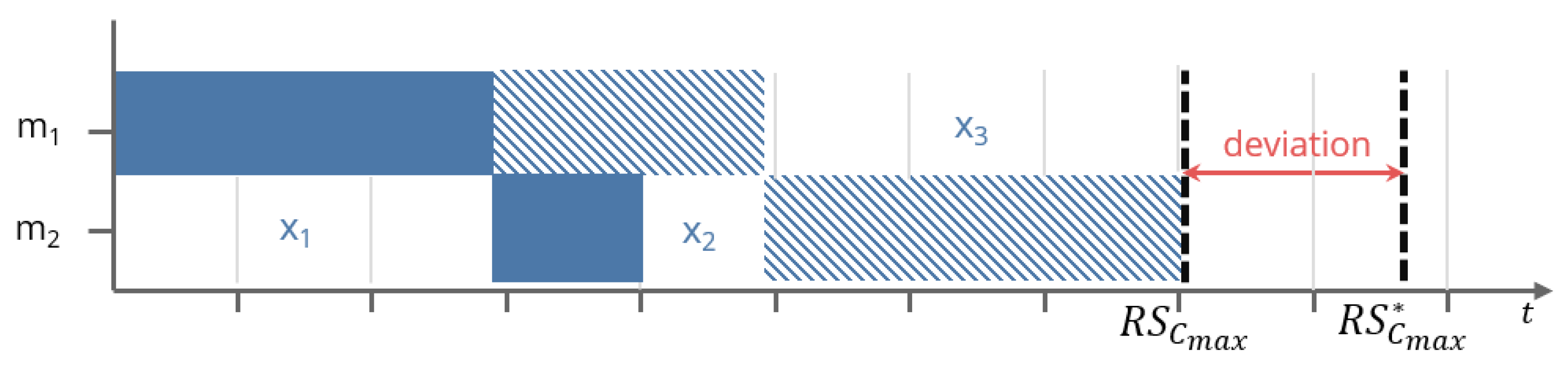
3.1. Idle Time Deviation

R and idle time deviations between RS and RS* are certainly related, which confirms $H_1$. It is to be assumed that $\forall o\in R{S}_O^{*}:o_e-o_s\approx o_E$. If $R\not\approx 0$, then the deviation between $R{S}_Z$ and $R{S}_Z^{*}$ is purely affected by idle times. Thus, the following equation precisely approximates R:

$$\begin{array}{c}\hfill R_{C_{max}}\approx \frac{\Delta X}{m}=\frac{1}{m}\left(\sum _{i=1}^{|R{S}_X|}R{S}_{x_i}-R{S}_{x_i}^{*}\right)\end{array}$$

(1)

It relativizes the sum of idle time deviations $\Delta X$ with regard to the number of machines m. A RMSE$<1\%$ could be obtained, which can be explained by measurement errors from MCE (for more information see

Table 2. Comparison of robustness prediction models (results after cross-validation).

Method	MSE	RMSE	MAE	MAPE
Equation (1) ($H_1$)	0.00004	0.0065	0.0050	0.0095
LR	0.00202	0.0450	0.0363	0.0683
Neural network	0.00283	0.0525	0.0408	0.0877
Gradient boosting	0.00292	0.0539	0.0404	0.0903
Random forest	0.00410	0.0639	0.0481	0.1099
Support vector machine	0.00428	0.0654	0.0536	0.1017

). Overlapping integrals $\lambda >0$ lead to a leverage effect in schedules with idle times or more than one machine: If the actual operation completion time $o_e$ lies inside an integral, it shifts and delays the successor operation ${\overrightarrow{o}}_k$ or ${\overrightarrow{o}}_j$, which recursively shifts its direct successors as well [3]. Thus, a cumulative displacement of critical path operations is the reason for $\Delta X\ne 0$. In other words: the more overlaps, the noisier $o_e$, $o_s$ but not $o_E$ [32], and thus the noisier the idle times between operations. To sum up, this finding suggests to include idle times and overlapping UPTs as features in the RMs. By accounting for these factors, the models may be better able to capture the complex dynamics of the system and provide more accurate predictions.

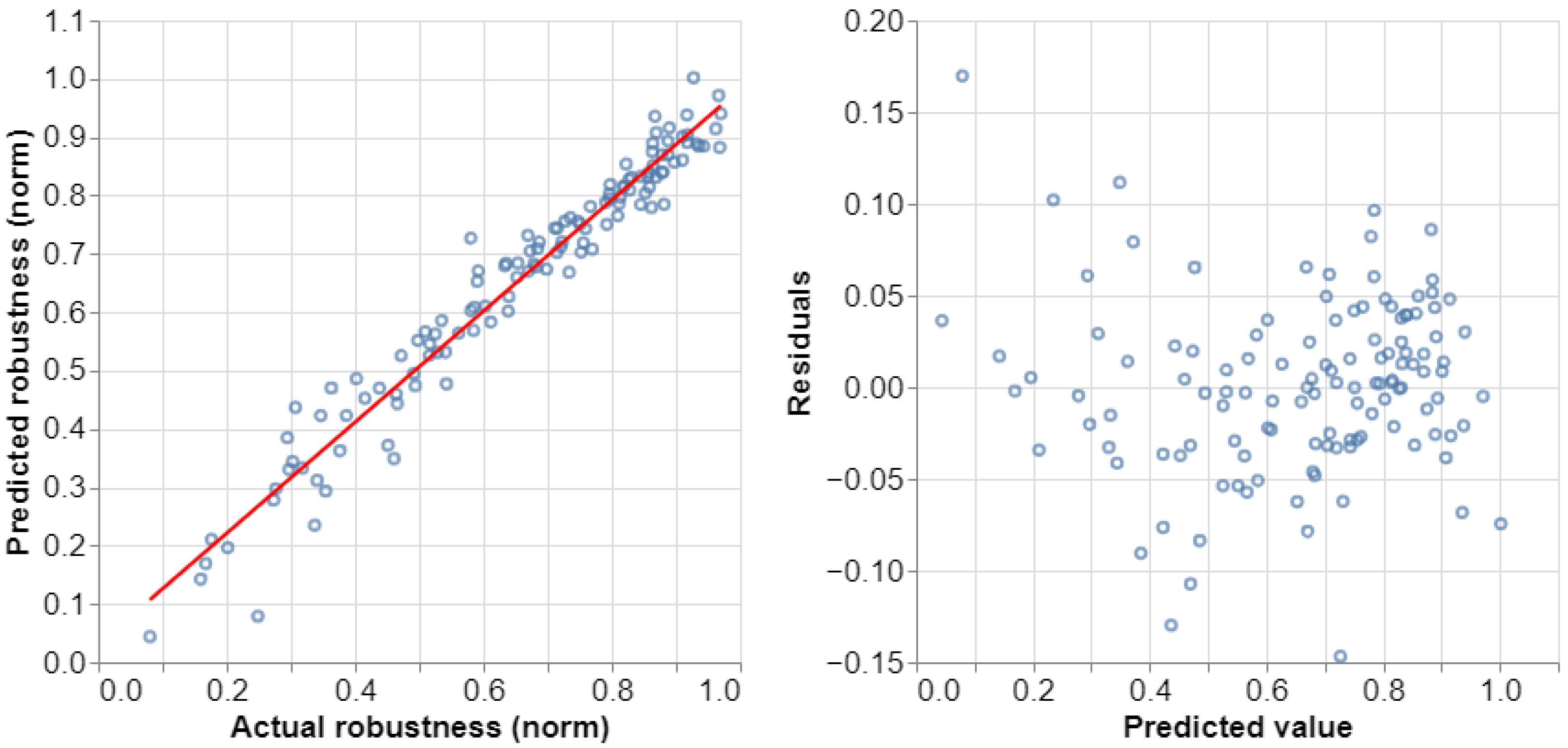
3.2. Regression Model Validation

$H_2$ could be confirmed: RMs were able to appropriately predict makespan robustness based on a priori information including overlapping integrals. Table 2 shows the summary statistics of validation results of the implemented ML models. According to the obtained scores, all ML models had low prediction errors and a high robustness to outliers. Thus, it can be inferred that RMs generally appear to be well suited for predicting robustness. Even if a hyperparameter search was conducted for the neural network, LR still had the highest accuracy. One possible explanation is that the data exhibit a linear structure, which is an advantage for LR models. In contrast, neural networks are more suitable for modeling complex nonlinear relationships [33].

To further examine the LR performance, Figure 4 displays a residual analysis. Although there are some minor outliers, the data points show a clear linear direction and a symmetric form with evenly distributed errors. No funnel shape or obvious nonlinear relationship can be observed in the residuals, which is is an indicator that there is no heteroscedasticity or other dependencies. If we now turn to the coefficients of the trained model, we observed that ${\omega }_{10}$ (coefficient $=1.12$) had the greatest influence on the prediction, which indicates a multicollinearity at first glance. Upon closer analysis, there is a high correlation with ${\omega }_{11}$ (coefficient $=-0.69$). However, without considering ${\omega }_{11}$ as a feature, the model’s predictions noticeably worsen. Therefore, both the mean total slack and its associated standard deviation are important features for prediction. Other important features were ${\omega }_4$ (coefficient $=-0.63$) and ${\omega }_1$ (coefficient $=0.44$), which confirms the association between overlapping UPTs, idle times and critical path operations. Overall, the analysis suggests that suitable features were selected to predict the makespan robustness. Moreover, the findings suggest that multiple different features are needed to define an accurate SM.

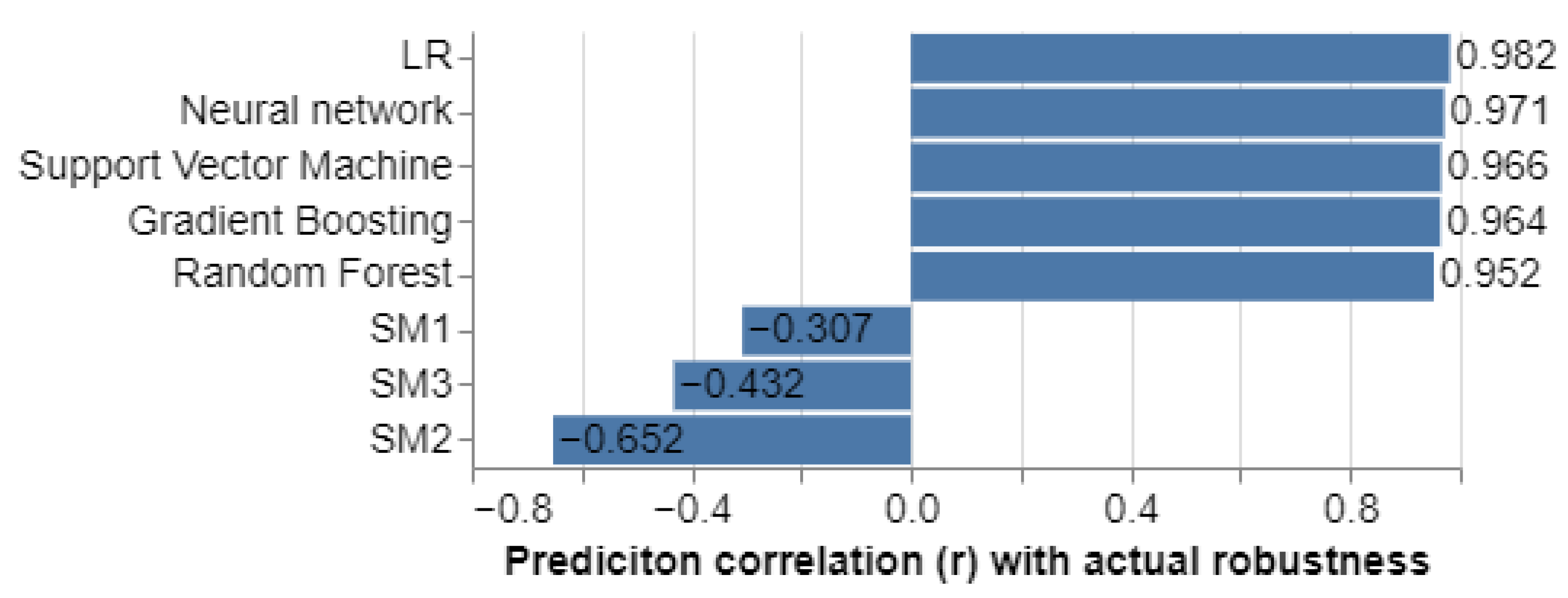
3.3. Surrogate Measure Benchmark

$H_3$ could be confirmed in the context of the considered test data: RMs obtain very high correlations with actual makespan robustness and clearly outperform SMs. The ML models were benchmarked against three widely used SMs. Traditionally, most surrogate measures are based on slack, and the importance of slack for robustness estimation was also confirmed in [20]. As mentioned in Section 1.3, recent developments in the field of surrogate measures are problem-specific and thus cannot be readily applied to this benchmark. Our first SM for robustness was the average slack measure introduced in [4] and utilized by many researchers such as [8,9,12,16,34] up to today. The proposed measure is given by

$$\begin{array}{c}\hfill S{M}_1=\frac{1}{|R{S}_o|}\sum _{o\in R{S}_o}{s}_o\end{array}$$

where $s_o$ denotes the total slack of operation o. Total slack is defined as the units of time an operation can be delayed without increasing the makespan. However, since operations on the same path in a schedule share total slack, summation of total slack of all operations could potentially overestimate the capability of the buffer [20]. In [34], the authors proposed the total sum of free slack, which is defined as the units of time an operation can be delayed without delaying the start of the next operation SM. It is calculated as follows:

$$\begin{array}{c}\hfill S{M}_2=\sum _{o\in R{S}_o}{f}_o\end{array}$$

where $f_o$ denotes the free slack of operation o. The third SM we used was also introduced by [34]. $S{M}_3$ is given by the weighted sum of total slack for each operation

$$\begin{array}{c}\hfill S{M}_3=\sum _{o\in R{S}_o}\frac{w_{o_k}}{w_{total}}{s}_o\end{array}$$

where $w_{o_k}$ describes the workload of the machine operation o that it is processed on, $w_{total}$ describes the total workload of all machines, and $s_o$ is again the total slack of operation o.

Since the introduced SMs do not try to estimate the actual robustness of a schedule, but try to correlate with it, a correlation analysis of the SMs and the predicted robustness values of the ML-algorithms was conducted. As shown in Figure 5, the predictions of the ML algorithms strongly correlate with the actual makespan robustness, which was an expected result given the results from the previous experiment. The SMs, on the other hand, have only a moderate negative correlation with actual robustness. A possible explanation for this outcome is that common SMs tend to focus on a limited number of variables to assess robustness, which may be an overly simplistic assumption. However, in the previous section, it was found that several factors associated with the critical path affect the robustness. This includes not only individual measures of slack times or workloads, but also more detailed features to describe the schedule and its uncertainties as comprehensively as possible. In the next section, the compared methods are applied to a new scenario beyond the provided test data. Here, we investigate how the different approaches affect the actual quality of generated RSs.

3.4. Application Study

To investigate the applicability and transferability of the RMs as well as their concrete advantages over SMs and MCEs, this experiment evaluates the proposed approach in the context of a typical robust scheduling procedure. We implemented a simulated annealing with research strategy (SARS) algorithm proposed by [17] to solve a robust PFS scheduling problem considering the constraints formulated in Section 1.1. The algorithm was executed for 100 iterations, and per iteration, a solution neighbor was generated by swapping the positions of two randomly selected jobs. The following multi-criteria objective function is defined for the synchronous minimization of the expected makespan and the makespan robustness:

$$\begin{array}{c}min{C}_{max}=\underset{o\in R{S}_O}{max}\left\{o_e\right\}\hfill \\ min{R}_{C_{max}}=\left\{\begin{array}{c}|R{S}_{C_{max}}-R{S}_{C_{max}}^{*}|,\mathrm{if}\mathrm{MCE}\mathrm{s}\mathrm{are}\mathrm{utilized}\mathrm{to}\mathrm{determine}\mathrm{robustness}\hfill \\ \left|PREDICT\right(RS\left)\right|,\mathrm{if}\mathrm{LR}\mathrm{is}\mathrm{utilized}\hfill \\ -S{M}_2,\mathrm{else}\hfill \end{array}\right.\hfill \end{array}$$

(2)

In terms of robustness evaluation, the specific value for Equation (2) can be determined by MCE, SM or by a RM. As $S{M}_2$ and LR exhibited the strongest correlations, they were selected as the models to be benchmarked. When selecting the best feasible solution, 80% priority (weight) was given to the robustness objective, and 20% was given to the makespan objective. In order to demonstrate the transferability of the method, we used a well-known test instance ($ta001$) introduced by [30] to evaluate the performance of the three methods. The instance consists of 20 jobs and 5 machines, and we modified it to include UPTs. Based on each operation processing time, we selected a random shape parameter $\alpha \in \{1.5,2,2.5,3,3.5,4,4.5,5\}$ and the scale parameter $\beta =5$ to generate a gamma distribution (see Section 2.3).

Figure 6 depicts a benchmark of the three methods in terms of the specified problem. In addition to LR and $S{M}_2$, MCEs were performed to varying extents. In one case, 200 stochastic simulations were conducted per creation of a neighbor solution, while in the other case, 400 simulations were conducted. Due to the 100 iterations of the SARS procedure, a total of 20,000 and 40,000 simulations had to be performed. For each method, 25 samples were collected to analyze the mean and variability of the obtained values. A closer inspection of the plots confirms the assumption that a traditional SM, while computationally efficient, yields relatively poor results. This applies to both the average values and the variance achieved. Particularly for the robustness values achieved, there are sometimes unacceptable outliers, which explain the moderate correlation observed in experiment 3 (see Section 3.2). On the other hand, MCEs provide significantly better schedules, but this comes at the cost of a large number of simulations. Especially when using extensive material flow simulations with computation times of several seconds per run, this is a crucial and potentially unacceptable hurdle. Another noteworthy observation is the varying robustness spread between 200 and 400 simulations per iteration. Doubling the number of simulations leads to higher precision and greater reliability of the method to minimize actual robustness. However, this is a critical tradeoff in terms of computation time.

If we now turn to LR, the benefits of the method become apparent in the figure. Utilizing ML models, it is possible to generate RSs that are close in quality to the MCE-based schedules with a minimum of computing time. Although the achieved makespan is slightly worse compared to the MCE-based method, the average achieved robustness is surprisingly even better. However, this initially unexpected result is understandable with regard to a slight model bias. One possible explanation in this context is that the model provides a rather pessimistic prediction of robustness. On the one hand, this leads to the generation of even more RSs. On the other hand, however, it also affects the conflicting objective of minimizing makespan, as displayed in the figure. The same pattern can also be observed between $MCE\times 200$ and $MCE\times 400$. Using fewer simulations results in a slightly less precise estimated robustness, but in comparison to $MCE\times 400$, it leads to a slightly better actual robustness and a slightly worse makespan. One possible solution to address this issue in this case is to use two plausible strategies. The first is to further improve the training of the RM to reduce the mentioned pessimism. Alternatively, the prioritization of the objectives could be adjusted in favor of minimizing makespan.

Overall, it has been confirmed that SMs generate significantly less optimal and less reliable schedules compared to what can be achieved with multivariate RMs. Thus, the results of this last experiment complement the results from the previous sections. In this specific scenario, it was possible to reconfirm $H_3$ from an application-oriented perspective. However, more scenarios must be investigated in future works.

4. Conclusions

This work employed RMs to predict makespan robustness for generic production schedules represented by DASGs and with the consideration of gamma-distributed UPTs. Within a computational study, three hypotheses $H_1,H_2,H_3$ could be confirmed: Overlapping uncertainty distributions on the critical path leas to a cumulative displacement of actual operation end times, which accordingly makes the idle time windows more noisy (see Section 3.1, $H_1$). This effect needs to be taken into account to construct feature vectors for ML models. In this manner, RMs and especially LR algorithms are suitable to accurately predict robustness with multiple a priori variables from the baseline DASG and are known before schedule realization or evaluation (see Section 3.2, $H_2$). Utilizing these models, well-known SMs could be significantly outperformed (see Section 3.3 and Section 3.4, $H_3$). Overall, the models offer a promising alternative to previous approaches such as inaccurate SMs and computationally intensive MCEs. In particular, they combine the advantages of both approaches: A well-trained model is able to anticipate the output of runtime-intensive simulations with a single prediction. If it is integrated into a optimization procedure, the complexity can be significantly reduced without major loss in solution quality. From a practical point of view, time-critical robust scheduling procedures could be executed in an even more resource-saving manner without the need of stochastic material flow simulations. This is particularly relevant in the context of rescheduling procedures that need to react quickly during daily operations to create a new RS. However, further research is necessary to evaluate the external validity of the method in other scenarios. The method must be tested with other scheduling models, uncertainty modelings, robustness or stability measures. Although we assume that our method can be applied to other distribution types, the effect of dynamic events such as machine failures must to be analyzed more closely. Moreover, it would also be interesting to investigate how the method performs on real-world production data. Consequently, the results of this study clearly motivate further research on this topic.

References

1. Pinedo, M.L. Scheduling, 4th ed.; Springer US: New York, NY, USA, 2012; p. 1. [Google Scholar] [CrossRef]
2. Rossi, F.L.; Nagano, M.S.; Sagawa, J.K. An effective constructive heuristic for permutation flow shop scheduling problem with total flow time criterion. Int. J. Adv. Manuf. Technol. 2016, 90, 93–107. [Google Scholar] [CrossRef]
3. Vela, C.R.; Afsar, S.; Palacios, J.J.; Gonzalez-Rodriguez, I.; Puente, J. Evolutionary tabu search for flexible due-date satisfaction in fuzzy job shop scheduling. Comput. Oper. Res. 2020, 119, 104931. [Google Scholar] [CrossRef]
4. Leon, J.V.; Wu, D.S.; Storer, R.H. Robustness measures and robust scheduling for job shops. IIE Trans. 1994, 26, 32–43. [Google Scholar] [CrossRef]
5. Davenport, A.J.; Gefflot, C.; Beck, J.C. Slack-based Techniques for Robust Schedules. In Proceedings of the Sixth European Conference on Planning (ECP-2001), Toledo, Spain, 12–14 September 2001. [Google Scholar]
6. Ouelhadj, D.; Petrovic, S. A survey of dynamic scheduling in manufacturing systems. J. Sched. 2008, 12, 417–431. [Google Scholar] [CrossRef]
7. Iglesias-Escudero, M.; Villanueva-Balsera, J.; Ortega-Fernandez, F.; Rodriguez-Montequín, V. Planning and Scheduling with Uncertainty in the Steel Sector: A Review. Appl. Sci. 2019, 9, 2692. [Google Scholar] [CrossRef]
8. Xiao, S.; Sun, S.; Jin, J.J. Surrogate measures for the robust scheduling of stochastic job shop scheduling problems. Energies 2017, 10, 543. [Google Scholar] [CrossRef]
9. Goren, S.; Sabuncuoglu, I. Robustness and stability measures for scheduling: Single-machine environment. IIE Trans. 2008, 40, 66–83. [Google Scholar] [CrossRef]
10. Shen, X.N.; Han, Y.; Fu, J.Z. Robustness measures and robust scheduling for multi-objective stochastic flexible job shop scheduling problems. Soft Comput. 2016, 21, 6531–6554. [Google Scholar] [CrossRef]
11. Liu, F.; Wang, S.; Hong, Y.; Yue, X. On the Robust and Stable Flowshop Scheduling Under Stochastic and Dynamic Disruptions. IEEE Trans. Eng. Manag. 2017, 64, 539–553. [Google Scholar] [CrossRef]
12. Sundstrom, N.; Wigstrom, O.; Lennartson, B. Conflict Between Energy, Stability, and Robustness in Production Schedules. IEEE Trans. Autom. Sci. Eng. 2017, 14, 658–668. [Google Scholar] [CrossRef]
13. Behnamian, J. Survey on fuzzy shop scheduling. Fuzzy Optim. Decis. Mak. 2015, 15, 331–366. [Google Scholar] [CrossRef]
14. Delgoshaei, A.; Ariffin, M.K.A.B.M.; Leman, Z.B. An Effective 4–Phased Framework for Scheduling Job-Shop Manufacturing Systems Using Weighted NSGA-II. Mathematics 2022, 10, 4607. [Google Scholar] [CrossRef]
15. Goyal, B.; Kaur, S. Flow shop scheduling-especially structured models under fuzzy environment with optimal waiting time of jobs. Int. J. Des. Eng. 2022, 11, 47. [Google Scholar] [CrossRef]
16. Xiao, S.; Wu, Z.; Dui, H. Resilience-Based Surrogate Robustness Measure and Optimization Method for Robust Job-Shop Scheduling. Mathematics 2022, 10, 4048. [Google Scholar] [CrossRef]
17. Grumbach, F.; Müller, A.; Reusch, P.; Trojahn, S. Robust-stable scheduling in dynamic flow shops based on deep reinforcement learning. J. Intell. Manuf. 2022. [Google Scholar] [CrossRef]
18. Soofi, P.; Yazdani, M.; Amiri, M.; Adibi, M.A. Robust Fuzzy-Stochastic Programming Model and Meta-Heuristic Algorithms for Dual-Resource Constrained Flexible Job-Shop Scheduling Problem Under Machine Breakdown. IEEE Access 2021, 9, 155740–155762. [Google Scholar] [CrossRef]
19. Minguillon, F.E.; Stricker, N. Robust predictive–reactive scheduling and its effect on machine disturbance mitigation. CIRP Ann. 2020, 69, 401–404. [Google Scholar] [CrossRef]
20. Zahid, T.; Agha, M.H.; Schmidt, T. Investigation of surrogate measures of robustness for project scheduling problems. Comput. Ind. Eng. 2019, 129, 220–227. [Google Scholar] [CrossRef]
21. Yang, Y.; Huang, M.; Wang, Z.Y.; Zhu, Q.B. Robust scheduling based on extreme learning machine for bi-objective flexible job-shop problems with machine breakdowns. Expert Syst. Appl. 2020, 158, 113545. [Google Scholar] [CrossRef]
22. Goren, S.; Sabuncuoglu, I.; Koc, U. Optimization of schedule stability and efficiency under processing time variability and random machine breakdowns in a job shop environment. Nav. Res. Logist. 2011, 59, 26–38. [Google Scholar] [CrossRef]
23. Himmiche, S.; Marangé, P.; Aubry, A.; Pétin, J.F. Robustness Evaluation Process for Scheduling under Uncertainties. Processes 2023, 11, 371. [Google Scholar] [CrossRef]
24. Jierula, A.; Wang, S.; OH, T.M.; Wang, P. Study on Accuracy Metrics for Evaluating the Predictions of Damage Locations in Deep Piles Using Artificial Neural Networks with Acoustic Emission Data. Appl. Sci. 2021, 11, 2314. [Google Scholar] [CrossRef]
25. Singh, U.; Rizwan, M.; Alaraj, M.; Alsaidan, I. A Machine Learning-Based Gradient Boosting Regression Approach for Wind Power Production Forecasting: A Step towards Smart Grid Environments. Energies 2021, 14, 5196. [Google Scholar] [CrossRef]
26. Chen, C.; Twycross, J.; Garibaldi, J.M. A new accuracy measure based on bounded relative error for time series forecasting. PLoS ONE 2017, 12, e0174202. [Google Scholar] [CrossRef] [PubMed]
27. Ratner, B. The correlation coefficient: Its values range between +1/−1, or do they? J. Target. Meas. Anal. Mark. 2009, 17, 139–142. [Google Scholar] [CrossRef]
28. Montaño, J.J.; Palmer, A.; Sesé, A.; Cajal, B. Using the R-MAPE index as a resistant measure of forecast accuracy. Psicothema 2013, 500–506. [Google Scholar] [CrossRef]
29. Yamashiro, H.; Nonaka, H. Estimation of processing time using machine learning and real factory data for optimization of parallel machine scheduling problem. Oper. Res. Perspect. 2021, 8, 100196. [Google Scholar] [CrossRef]
30. Taillard, E. Benchmarks for basic scheduling problems. Eur. J. Oper. Res. 1993, 64, 278–285. [Google Scholar] [CrossRef]
31. Jacoboni, C.; Lugli, P. The Monte Carlo Method for Semiconductor Device Simulation; Springer: Vienna, Austria, 1989. [Google Scholar] [CrossRef]
32. Kuroda, M.; Wang, Z. Fuzzy job shop scheduling. Int. J. Prod. Econ. 1996, 44, 45–51. [Google Scholar] [CrossRef]
33. Goodfellow, I.; Bengio, Y.; Courville, A. Deep Learning; MIT Press: Cambridge, MA, USA, 2016; pp. 164–199. Available online: http://www.deeplearningbook.org (accessed on 15 March 2023).
34. Xiong, J.; Xing, L.N.; Chen, Y.W. Robust scheduling for multi-objective flexible job-shop problems with random machine breakdowns. Int. J. Prod. Econ. 2013, 141, 112–126. [Google Scholar] [CrossRef]
Figure 1. Exemplary feasible solutions to (flexible) PFS, FS and JS problems with three jobs and two machines (Gantt and DASG representation).
Processes 11 01267 g001
Figure 2. Exemplary schedule with two jobs and two machines (Gantt representation).
Processes 11 01267 g002
Figure 3. Two subsequent operations on a machine m k . With a probability of p d , the machine predecessor operation o k is shifted to the right on the time axis. Expected shift: E d .
Processes 11 01267 g003
Figure 4. Residual analysis of the LR model (best identified RM) with 125 test samples.
Processes 11 01267 g004
Figure 5. Correlation benchmark of selected RMs and SMs. Key finding: RMs clearly outperform SMs in the approximation of C m a x robustness.
Processes 11 01267 g005
Figure 6. Comparing RSs generated by LR, S M 2 and MCE integrated into a SARS algorithm.
Processes 11 01267 g006