Article

The Application of Hyperspectral Images in the Classification of Fresh Leaves’ Maturity for Flue-Curing Tobacco

1
College of Tobacco, Henan Agriculture University, Zhengzhou 450002, China
2
Sichuan Tobacco Company, Chengdu 610000, China
3
Qujing Tobacco Company of Yunnan Province, Qujing 655000, China
*
Author to whom correspondence should be addressed.
Processes 2023, 11(4), 1249; https://doi.org/10.3390/pr11041249
Submission received: 8 March 2023 / Revised: 4 April 2023 / Accepted: 17 April 2023 / Published: 18 April 2023

Abstract

:
The maturity of tobacco leaves directly affects their curing quality. However, no effective method has been developed for determining their maturity during production. Assessment of tobacco maturity for flue curing has long depended on production experience, leading to considerable variation. In this study, hyperspectral imaging combined with a novel algorithm was used to develop a classification model that could accurately determine the maturity of tobacco leaves. First, tobacco leaves of different maturity levels (unripe, under-ripe, ripe, and over-ripe) were collected. ENVI software was used to remove the hyperspectral imaging (HSI) background, and 11 groups of filtered images were obtained using Python 3.7. Finally, a full-band-based partial least-squares discriminant analysis (PLS-DA) classification model was established to identify the maturity of the tobacco leaves. In the calibration set, the model accuracy of the original spectrum was 88.57%, and the accuracy of the de-trending, multiple scattering correction (MSC), and standard normalization variable (SNV) treatments was 91.89%, 95.27%, and 92.57%, respectively. In the prediction set, the model accuracy of the de-trending, MSC, and SNV treatments was 93.85%, 96.92%, and 93.85%, respectively. The experimental results indicate that a higher model accuracy was obtained with the filtered images than with the original spectrum. Because of the higher accuracy, de-trending, MSC, and SNV treatments were selected as the candidate characteristic spectral bands, and a successive projection algorithm (SPA), competitive adaptive reweighted sampling (CASR), and particle swarm optimization (PSO) were used as the screening methods. Finally, a genetic algorithm (GA), PLS-DA, line support vector machine (LSVM), and back-propagation neural network (BPNN) classification and discrimination models were established. The combination SNV-SPA-PLS-DA model provided the best accuracy in the calibration and prediction sets (99.32% and 98.46%, respectively). Our findings highlight the efficacy of using visible/near-infrared (ViS/NIR) hyperspectral imaging for detecting the maturity of tobacco leaves, providing a theoretical basis for improving tobacco production.

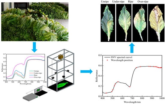
Graphical Abstract

1. Introduction

The flue curing of tobacco (Nicotiana tabacum L.) plants has greatly improved tobacco farmers’ income [1,2,3,4,5]. Tobacco production comprises many steps, including breeding, cultivation, harvesting, curing, and grading [6,7,8,9]. For the harvesting step, maturity is the most important indicator for determining whether tobacco leaves are ready for flue curing [10,11]. Using immature leaves or leaves at various maturity levels increases the difficulty of curing and reduces the quality of flue-cured tobacco leaves, resulting in great economic losses [12,13,14]. However, the assessment of tobacco maturity depends mainly on individual experience, and errors are introduced due to variations in levels of experience [5]. Consequently, establishing a harvest maturity standard was challenging. Therefore, developing an objective evaluation method to determine the maturity of tobacco leaves is highly desirable to improve tobacco production.
Hyperspectral imaging (HSI) technology has been utilized by an increasing number of agricultural experts to resolve problems in crop production, food safety, crop maturity, meat freshness, and other fields in recent years [15,16,17,18]. Yuan et al. [19] reported a visible/near-infrared (ViS/NIR) HIS system for classifying jujube internal bruises over time, and showed that this rapid and nondestructive technique could identify bruising time with 100% accuracy. Ke et al. [20] developed an HSI method for the nondestructive determination of volatile oil and moisture content and the discrimination of geographical origins of Zanthoxylum bungeanum Maxim. Yang et al. [21] reported a classification accuracy of 75.50% for an integrated convolutional neural network (CNN) model for estimating corn yield classification based on HSI and RGB images. Liu et al. [22] successfully proposed a novel framework that combines hyperspectral imaging (HSI) and deep learning techniques for plant image classification. The best accuracy measured for the models was 0.834.
Despite the progress made, most previous studies used only the original hyperspectral image without modifications. On the one hand, a lot of noise is generated during the acquisition of hyperspectral images due to the noise generated by the instrument itself and the external environment, as well as interference from light scattering [23], and on the other hand, original hyperspectral images comprise many narrow spectral bands, leading to a large amount of repeated information in the adjacent bands. Hyperspectral image data have high dimensionality and collinearity [19]. When applying an original hyperspectral image to experimental or production practice, hundreds of bands of data exist, which increases the computational burden calculation in the model-building process, seriously hindering the popularization and application of the model [24,25].Therefore, we need to effectively eliminate collinearity between variables, extract useful information from overlapping information, and minimize the number of variables and complexity of models to improve the efficiency and speed of modeling.Nevertheless, filtering transformation and characteristic wavelength screening have a good effect on reducing the multidimensionality and high collinearity of hyperspectral data, which could improve the speed of the model [26,27,28]. In many studies, several filtering methods, such as multiple scattering correction (MSC), standard normalization variable (SNV), and Gaussian filter (GF), have been used to filter the original hyperspectral image, while particle swarm optimization (PSO), competitive adaptive reweighted sampling (CARS), and successive projection algorithm (SPA) have been used to select characteristic wavelengths.
Concerning tobacco, researchers have used HSI to analyze the color and location features of tobacco [29] to rapidly and nondestructively predict nicotine and chlorophyll contents [30] and photosynthetic capacity [31] and quantitate tobacco chemical composition [25]. Focusing on the classification of tobacco maturity, Chen et al. [5] successfully used near-infrared spectroscopy to discriminate between the different maturity levels of fresh tobacco leaves. However, this technique relies on a high computational effort that increases the processing workload. Therefore, we postulate that it would be a wise solution to establish an efficient and accurate maturity recognition model for flue-cured tobacco by using the method of filtering and transforming the original spectra and screening the characteristic spectra. In the present study, we developed a new methodology to determine the maturity of tobacco leaves using hyperspectral technology. This new method has a lower computational burden than current methods while producing more accurate results. This proposed method is expected to replace the traditional method of classifying tobacco maturity grade, providing an auxiliary means for objective classification of tobacco maturity and reducing the difficulty of tobacco curing.

2. Materials and Methods

2.1. Sample Preparation

Tobacco leaves were obtained from Luoyang, Henan Province, China, in 2021. A total of 213 tobacco samples were collected for this study. Experts who had been engaged in flue-cured tobacco leaf production for a long time were invited to evaluate the maturity level of all samples and label them according to four maturity stages (unripe, under-ripe, ripe, and over-ripe), as shown in Table 1. There were 36 unripe, 43 under-ripe, 91 ripe, and 53 over-ripe tobacco leaves. Hyperspectral images of all samples were obtained within 2 h.

2.2. Acquisition of Hyperspectral Images

Hyperspectral images were acquired using a HSI system (GaiaField-V10E, Jiangsu Dualix Spectral Imaging Technology Co., Ltd., Wuxi City, Jiangsu, China). The spectral range was 400–1000 nm. The number of bands in the hyperspectral images was 256. Data acquisition and management were conducted using SpecView software 5.3.1 (Jiangsu Dualix Spectral Imaging Technology Co., Ltd., Wuxi City, Jiangsu, China). A clear image was captured using an exposure time of 12 ms. The distance between the sample and the camera was 120 cm. Four 200 W/220 V halogen lamps were used as the light source. A schematic is shown in Figure 1.

2.3. Hyperspectral Image Correction

During hyperspectral image acquisition, dark currents and uneven illumination lead to noise in the collected images [32]. Therefore, the hyperspectral image must be corrected using the white reference image Iwhite (obtained from the standard white plate scan) and the black reference image Idark (obtained by covering the lens without illumination). The corrected image R was transformed from raw hyperspectral image I based on Equation (1):
R = I I d a r k I w h i t e I d a r k

2.4. Extraction of Spectral and Image Data

To effectively extract the spectral and image data from the object, ENVI5.3.1 (Research System Inc., Boulder, CO, USA) software was used to mask and select the region of interest (ROI) in all sample images. The ROI was used to remove invalid backgrounds from the hyperspectral image. The mean spectral values of the removed background images were then calculated. Spectral data were extracted and preprocessed using Python 3.7.
In order to reduce the high dimensionality and collinearity of the hyperspectral image for further data analysis and modeling, it needed to be preprocessed. In this experiment, baseline, de-trending, MSC, normalization, orthogonal signal correction (OSC), Savitzky–Golay (SG), SNV, spectroscopic transformation (ST), GF, moving average (MA), and median filter (MF) methods were used to filter the original hyperspectral images. Baseline and ST can effectively block image noise [23]; de-trending is primarily used to eliminate baseline drift of diffuse reflections [17]; normalization unifies the spectral values of each image element to the overall average luminance level to reduce luminance differences [23]; MSC and SNV are mainly used for light scattering correction and aim to improve the accuracy of spectral data [23]; OSC is used to filter out noise from the raw data and to ensure that the information filtered out is not relevant to the information to be measured [19]; SG is mainly used to eliminate random noise [23]; GF eliminates Gaussian noise and is widely used in image processing for noise reduction [17]; MA can filter out high-frequency noise [17]; MF effectively blocks image noise, greatly reduces the blurring of image edges, and is better at handling slightly dense noise points [17].

2.5. Data Analysis

PLS-DA models [33] were used to analyze the filtered and original hyperspectral images. Then, high-accuracy image data were collected. Finally, to effectively eliminate collinearity between variables, minimize the complexity of the model variables, and improve the efficiency and speed of modeling, the SPA [34], PSO [35], and CARS [36] algorithms were used to obtain the characteristic wavelengths of the selected image from step 2. Finally, the GA [37], PLS-DA, LSVM [38], and BPNN [39] models were used to analyze the characteristic wavelengths of the hyperspectral images.

2.6. Analytical Software

The invalid background of the hyperspectral images was removed using ENVI5.3.1. Image filtering, characteristic wavelength selection, and construction of the analytical model were carried out in Python 3.7. The graphs were created using Excel 2010.

3. Results

3.1. Image Analysis

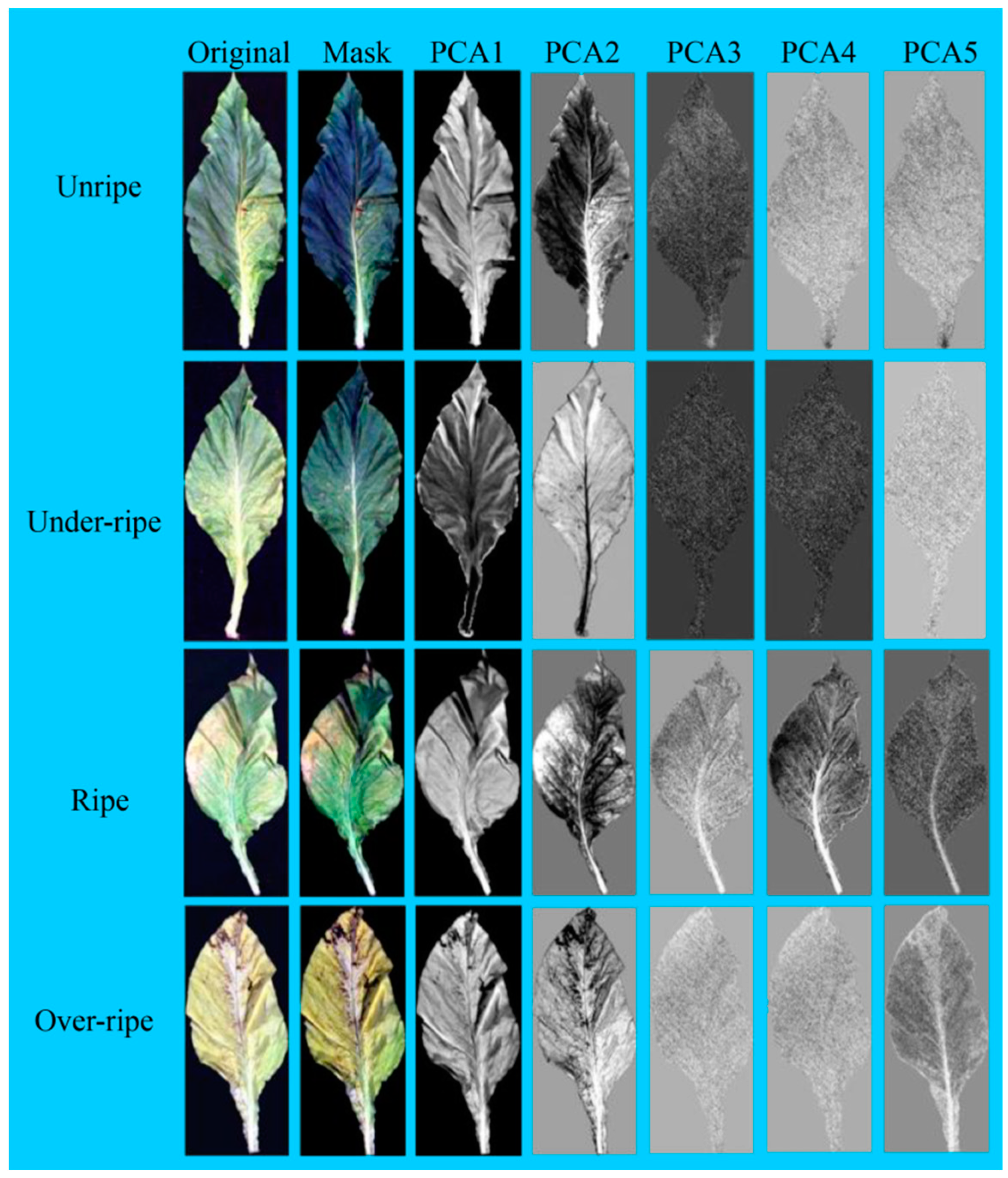
The ENVI software was used to mask the images of tobacco and remove the image background. As shown in Figure 2, the background image can be easily removed from the ROI. Principal component analysis (PCA) was performed on the masked images. The top 5 images of the 256 principal component images were then obtained. The results show that the color and principal components of tobacco leaves clearly differed among maturity levels and that the tobacco leaves changed from green to yellow as they matured.

3.2. Spectra Analysis

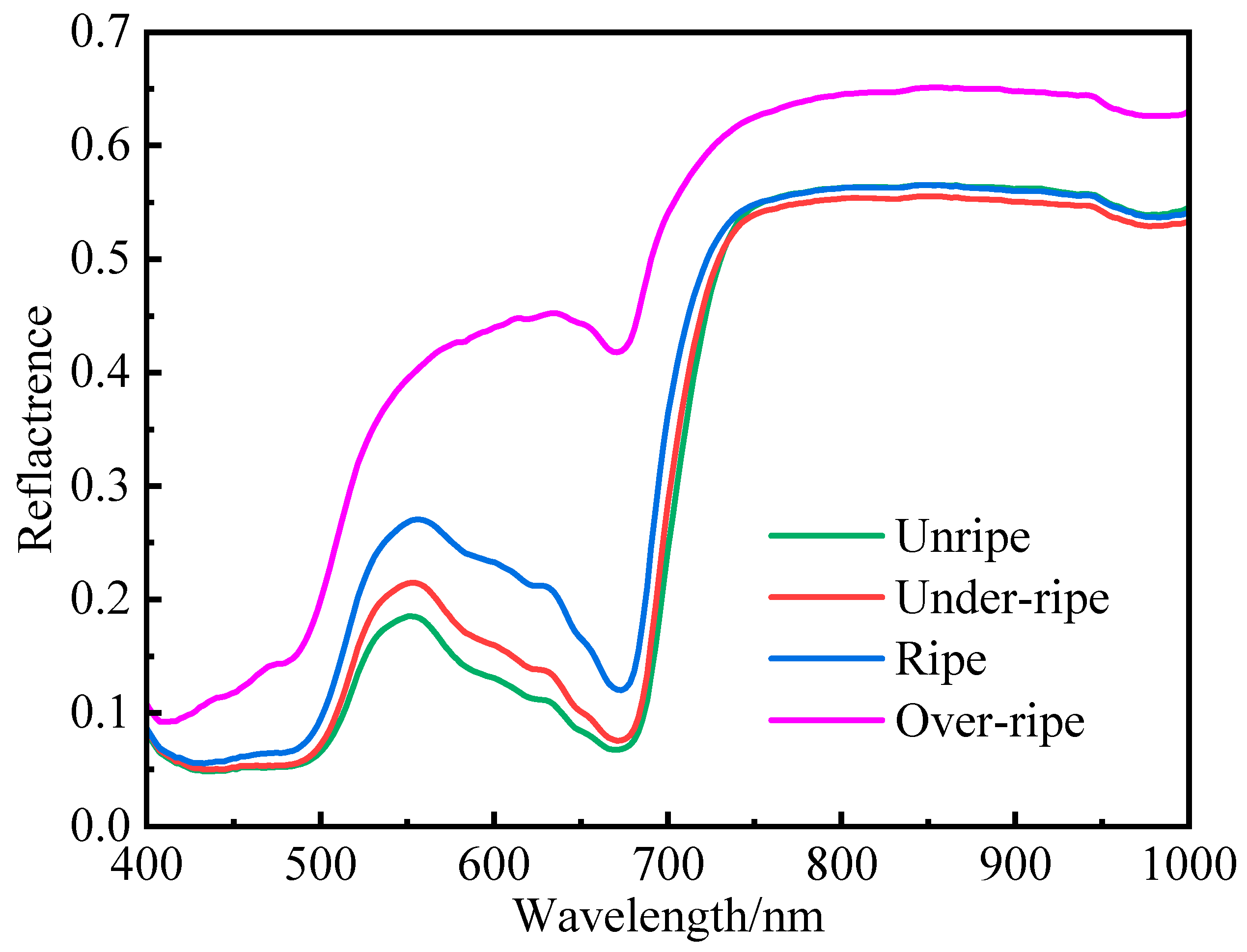
The spectral curves of tobacco leaves at different maturity levels are shown in Figure 3. Leaves at all maturity levels showed the same trend and had an absorption peak at 680 nm. In the range of 450–750 nm, the spectral reflectance of fresh tobacco leaves at different maturity levels followed the order over-ripe > ripe > under-ripe > unripe.

3.3. Filter Processing of Images

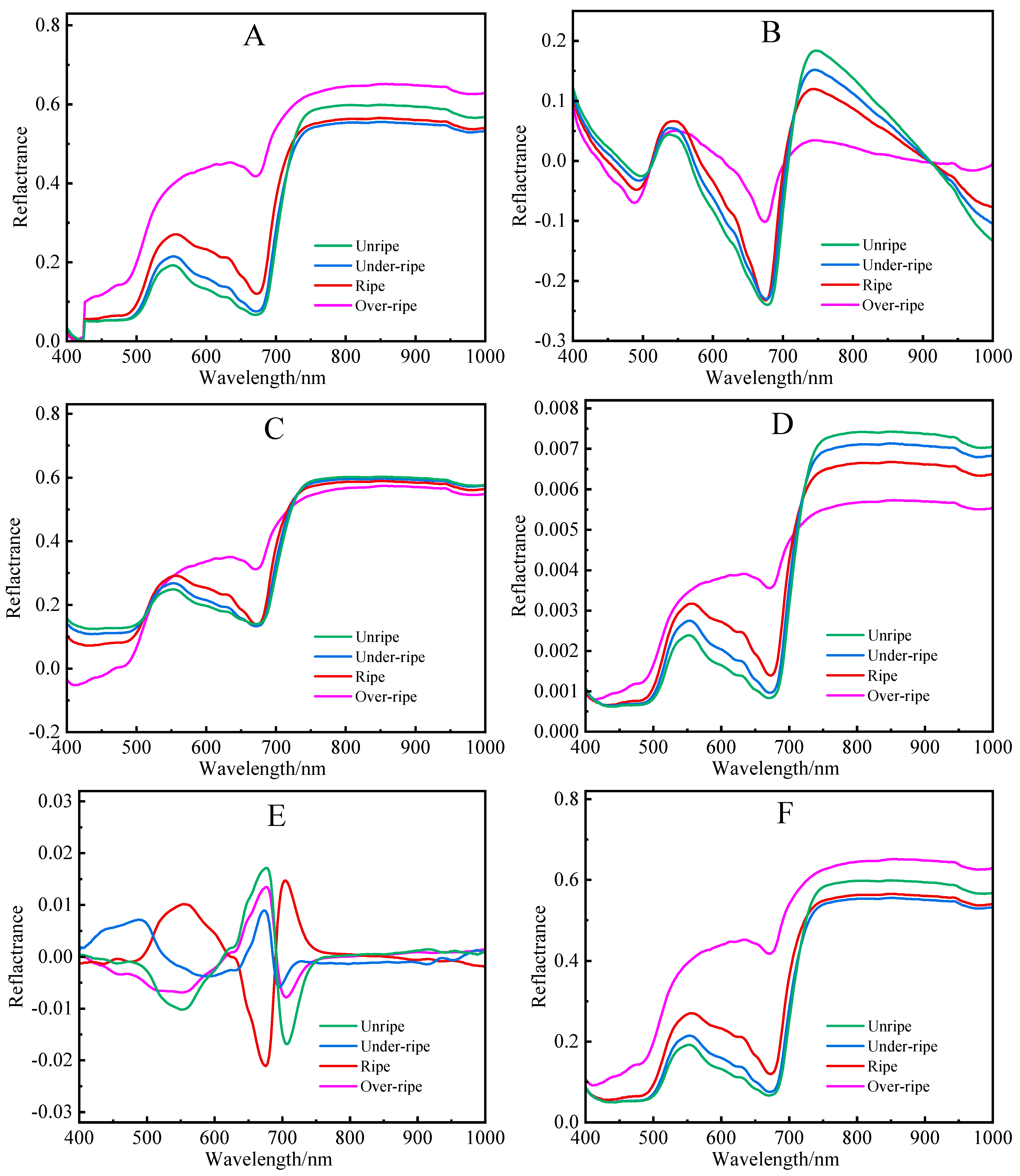
The original spectra were pretreated using the baseline, de-trending, MSC, normalize, OSC, SG, SNV, spectroscopic transformation, GF, MA, and MF methods, and the spectral curves obtained with the different pretreatments are shown in Figure 4. The trend of the original spectral curves differed from that of the filtered curves modified via de-trending, MSC, normalization, OSC, SNV, and spectroscopic filtering methods. However, the trends of the other filtered spectral data were more similar to those of the source spectra. Furthermore, with the exception of the OSC filtering treatment, the spectral trends of fresh tobacco leaves in the over-ripe grades differed significantly from those in the other maturity grades.

3.4. PLS-DA of Tobacco Leaf Images

Before establishing the PLS-DA classification model, the tobacco leaf samples were randomly assigned to two groups at a ratio of 7:3. From the samples, 70% were used as the calibration set, and the remaining 30% were used as the prediction set (30%). The allocation results are listed in Table 2, and the classification results of PLS-DA for the original and filtered spectra are shown in Table 3. In the calibration sets, the model accuracy of the original spectra was 87.84%. The model accuracies of the de-trending, MSC, and SNV spectra were 91.89%, 95.27%, and 92.57%, respectively, which are 4.05%, 7.43%, and 4.73% higher, respectively, than those of the original. The model accuracy of the other filtered images was lower than that of the original image. In the prediction set, the model accuracy of the original spectra was 92.31% and that of de-trending, MSC, and SNV spectra was 01.54%, 4.61%, and 1.54% higher at 93.85%, 96.92%, and 93.85%, respectively. However, the model accuracy of the other eight filtering methods was lower than that of the original method. In the calibration and prediction sets, the model accuracy of de-trending, MSC, and SNV spectra were always higher than that of the original. Therefore, these spectra can be used for screening characteristic spectral bands.

3.5. Selection of Characteristic Spectral Wavelengths

3.5.1. De-Trending

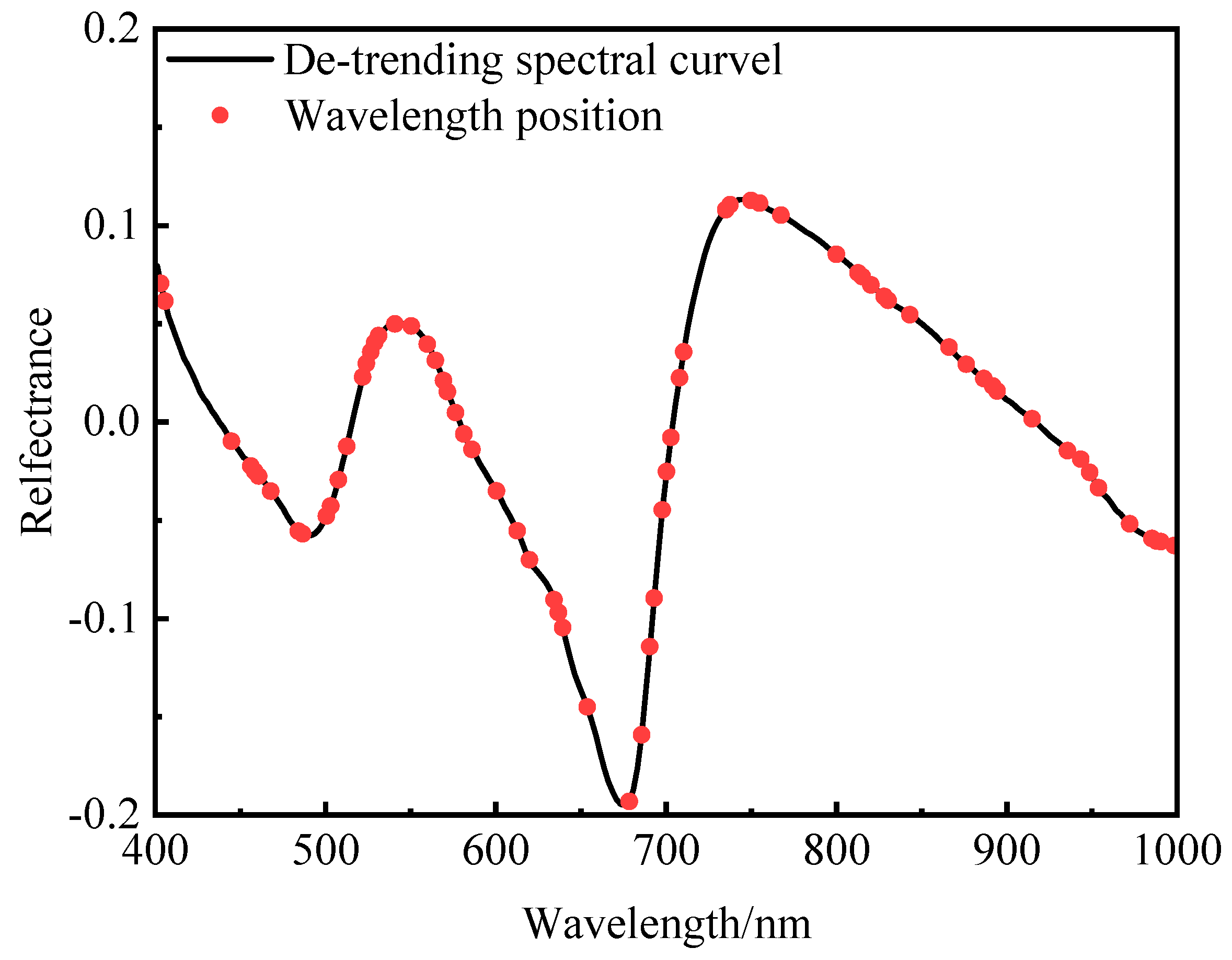
Seven characteristic spectral bands were selected using the SPA. These were 410.1, 510.0, 517.1, 531.3, 555.0, 610.1, and 941.0 nm (Figure 5). When the PSO algorithm was used to screen the characteristic spectral bands, 70 bands were selected. These were 403.3, 405.6, 444.7, 456.3, 458.6, 460.9, 467.9, 484.2, 486.6, 500.6, 503.0, 507.7, 512.4, 521.8, 524.2, 526.6, 528.9, 531.3, 540.8, 550.3, 559.8, 564.6, 569.3, 571.7, 576.5, 581.3, 586.1, 600.5, 612.6, 619.8, 634.3, 636.8, 639.2, 653.8, 678.3, 685.6, 690.5, 693.0, 697.9, 700.4, 702.9, 707.8, 710.3, 735.0, 737.5, 750.0, 755.0, 767.5, 800.1, 812.8, 815.3, 820.3, 828.0, 830.5, 843.2, 866.2, 876.4, 886.7, 891.8, 894.4, 915.0, 935.8, 943.6, 948.8, 954.0, 972.3, 985.4, 988.0, 990.6, and 998.5 nm (Figure 6). Using the CARS algorithm, 42 bands were selected. These were 414.7, 435.4, 449.3, 451.6, 458.6, 463.3, 495.9, 498.3, 507.7, 517.1, 519.5, 526.6, 531.3, 555, 605.3, 607.7, 612.6, 619.8, 673.4, 720.2, 737.5, 740, 745, 787.5, 858.5, 863.6, 873.9, 879, 886.7, 930.6, 948.8, 961.8, 964.4, 967, 972.3, 977.5, 982.7, 985.4, 988, 990.6, 995.9, and 998.5 nm (Figure 7).

3.5.2. Standard Normalization Variable (SNV)

In total, 22 bands were selected when using the SPA to screen the characteristic spectral bands. These were 437.8, 493.6, 505.3, 519.5, 528.9, 555.0, 675.8, 742.5, 782.5, 868.7, 884.1, 915.0, 930.6, 941.0, 951.4, 961.8, 969.6, 982.7, 988.0, 990.6, 993.2, and 998.5 nm (Figure 8). Using the PSO algorithm, 86 bands were selected. These were 401.0, 403.3, 423.9, 426.2, 433.1, 437.8, 442.4, 458.6, 460.9, 463.3, 470.2, 472.6, 474.9, 486.6, 493.6, 495.9, 498.3, 503.0, 517.1, 519.5, 521.8, 526.6, 559.8, 564.6, 586.1, 588.5, 602.9, 605.3, 615.0, 631.9, 634.3, 636.8, 646.5, 653.8, 666.0, 668.5, 673.4, 683.2, 695.5, 707.8, 710.3, 720.2, 722.6, 727.6, 730.1, 735.0, 740.0, 747.5, 760.0, 765.0, 782.5, 787.5, 790.1, 792.6, 800.1, 805.2, 815.3, 817.8, 825.4, 828.0, 830.5, 838.1, 843.2, 855.9, 858.5, 863.6, 866.2, 868.7, 871.3, 879.0, 884.1, 899.5, 909.9, 917.6, 925.4, 928.0, 935.8, 938.4, 941.0, 948.8, 964.4, 980.1, 982.7, 990.6, 993.2, and 998.5 nm (Figure 9). When the CARS algorithm was used to screen the characteristic spectral bands, 34 bands were selected. These were 421.6, 435.4, 456.3, 458.6, 498.3, 510, 512.4, 517.1, 519.5, 526.6, 533.6, 612.6, 617.4, 673.4, 742.5, 755, 787.5, 795.1, 805.2, 815.3, 822.9, 825.4, 835.6, 873.9, 886.7, 920.2, 933.2, 935.8, 943.6, 948.8, 956.6, 967, 977.5, and 982.7 nm (Figure 10).

3.5.3. Multiple Scattering Correction (MSC)

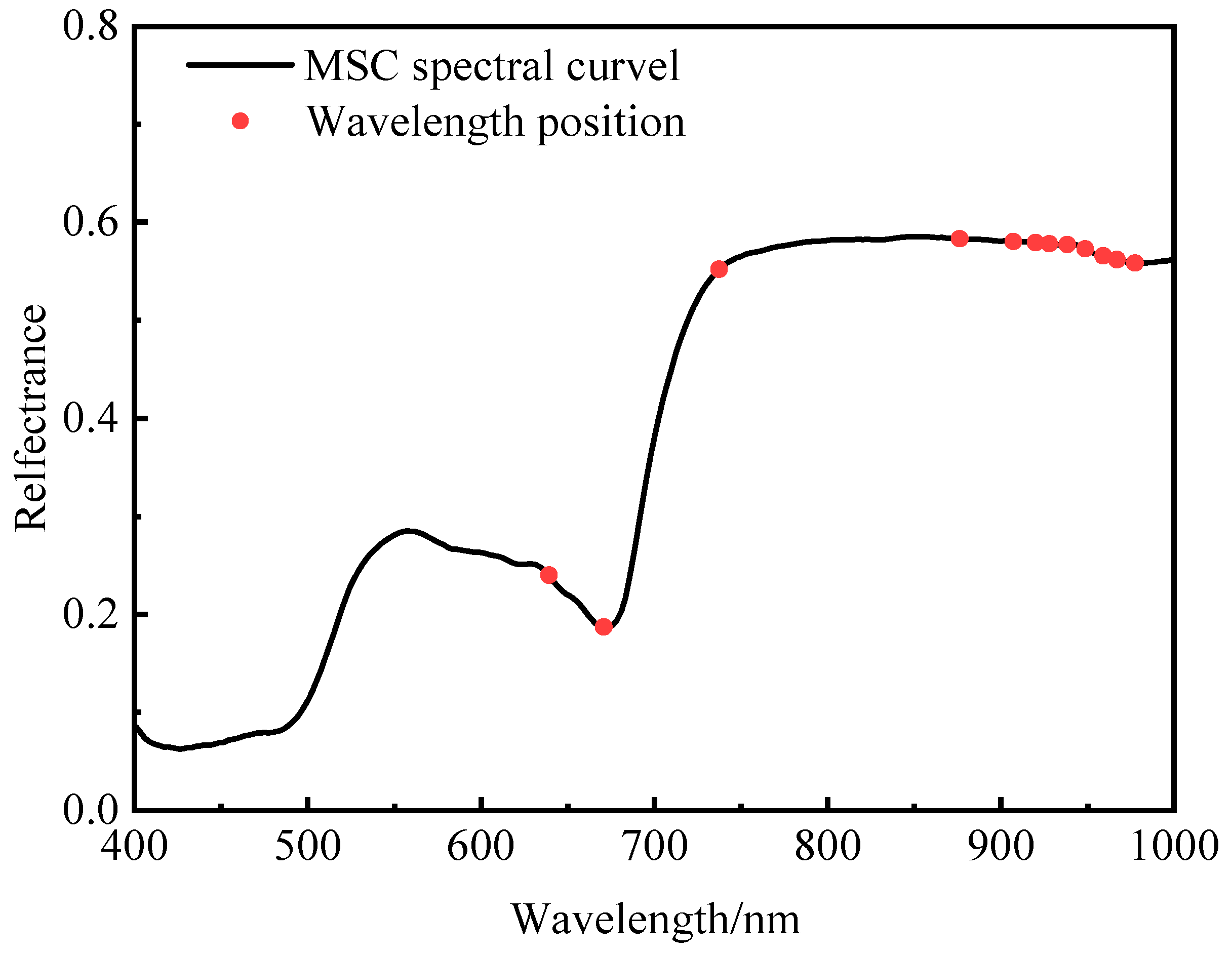
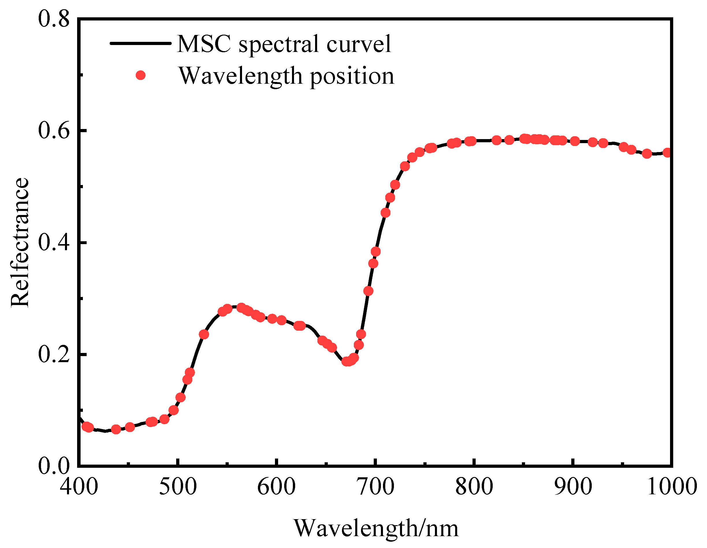
In total, 12 bands were selected using the SPA. These were 639.2, 670.9, 737.5, 876.4, 907.3, 920.2, 928, 938.4, 948.8, 959.2, 967, and 977.5 nm (Figure 11). The PSO algorithm selected 66 bands. These were 407.8, 410.1, 437.8, 451.6, 472.6, 474.9, 486.6, 495.9, 503.0, 510.0, 512.4, 526.6, 545.5, 550.3, 564.6, 569.3, 571.7, 578.9, 583.7, 595.7, 605.3, 622.2, 624.6, 646.5, 651.4, 656.2, 670.9, 673.4, 675.8, 678.3, 683.2, 685.6, 693.0, 697.9, 700.4, 707.8, 710.3, 715.2, 720.2, 730.1, 737.5, 740.0, 745.0, 755.0, 757.5, 777.5, 782.5, 795.1, 797.6, 822.9, 835.6, 850.8, 861.1, 863.6, 866.2, 871.3, 881.5, 884.1, 889.3, 902.1, 920.2, 930.6, 951.4, 959.2, 974.9, and 995.9 nm (Figure 12). The CARS algorithm selected 41 bands. These were 433.1, 437.8, 458.6, 495.9, 498.3, 507.7, 510, 512.4, 517.1, 519.5, 526.6, 528.9, 533.6, 555, 562.2, 612.6, 615, 617.4, 6 39.2, 658.7, 683.2, 742.5, 777.5, 785, 787.5, 795.1, 815.3, 817.8, 822.9, 825.4, 835.6, 873.9, 879, 886.7, 930.6, 935.8, 948.8, 956.6, 977.5, 982.7, and 990.6 nm (Figure 13).

3.6. Classification Results Using the Characteristic Wavelengths

The GA, PLS-DA, LSVM, and BP model results for classifying the characteristic wavelengths are shown in Table 4. The SNV-SPA-PLS-DA model provided the highest accuracy (99.32%) in the calibration set. The SNV-PSO-PLS-DA, MSC-SPA-PLS-DA, and MSC-PSO-PLS-DA models all achieved an adequate accuracy rate of 96% or more, which is slightly lower than that of SNV-SPA-PLS-DA. The accuracy of the other models was relatively low. In the prediction set, SNV-SPA-PLS-DA provided the highest accuracy at 98.46%, while the accuracies of SNV-PSO-PLS-DA, MSC-SPA-PLS-DA, and MSC-PSO-PLS-DA models were all less than 96%. The accuracy of the other models was relatively low. Therefore, the SNV-SPA-PLS-DA model had the highest accuracy, and the SNV-SPA-PLS-DA model could quickly and accurately identify the maturity of fresh tobacco leaves.

3.7. Classification Results of Tobacco Leaves of Different Maturities Using SVN-SPA-PLS-DA

Table 5 shows the confusion matrices of tobacco leaves at various levels of maturity obtained using the SNV-SPA-PLS-DA model. The classification accuracy at the over-ripe level was 97.14% and 95% in the calibration sets and prediction sets, respectively, and one tobacco leaf at this level was misclassified as ripe in both sets. The calibration and prediction sets could classify the remaining levels at 100% accuracy.

4. Discussion

Tobacco leaf maturity is an important factor during the production of tobacco [5,13]. Nowadays, there are mainly two strategies used to ensure the maturity of tobacco leaves in large tobacco-producing countries: one is to change agronomic methods by studying the ripening mechanism of tobacco leaves [40], and the other is to accurately assess the maturity of tobacco leaves and develop efficient curing technologies [5,10]. However, because the growth of tobacco is greatly affected by the environment, the first strategy is somewhat passive. The method developed in this study is efficient and accurate and not limited by the ecological environment of tobacco fields.
In this study, except for the OSC filtering, both the original spectral data and the other filtered spectral data showed a large difference between the over-ripe and ripe grades and the under-ripe and unripe grades, while the trends of under-ripe, ripe, and unripe were basically the same. This is mainly due to the fact that in the visible-light range, the chlorophyll of plant leaves has a strong light absorption capacity [41]; as fresh tobacco leaves gradually age, the chlorophyll content continues to decrease, and their light absorption capacity gradually weakens.
It was found that one sample was incorrectly classified using the SNV-SPA-PLS-DA model. The main reason for this is that the metabolism of tobacco leaf is a continuous process; therefore, the changes in the properties of the tobacco leaf are also continuous. Ripe and over-ripe are two adjacent maturity levels of fresh tobacco leaves that may have more similarity in color, moisture, and other components between them, and therefore their spectral characteristics are similar and more distinct. This provides some reference for further optimization of our model.
Chen et al. directly used 512 spectral bands of the original spectrum to model and identify the maturity of fresh tobacco leaves, with a maximum accuracy of 97.31% [5], while we only used 22 spectral bands to construct a fresh tobacco leaf maturity recognition model, and its accuracy reached 98.46%. This is mainly because we reduced the collinearity of hyperspectral data through filtering transformation, extracted more effective information, and reduced the calculation amount of the model by filtering the characteristic spectrum [42]. This technique reduces the computation requirements of the model, improves the recognition efficiency, and increases the probability of the technology being popularized and applied. However, since the number of samples was only 213 in this study, the accuracy of the model could be further improved by obtaining more sample data.

5. Conclusions

We have successfully established a novel algorithm for identifying the maturity of tobacco leaves. De-trending, MSC, and SNV were selected as the optimized filtering methods owing to their high accuracy. SPA and PSO were used to select the characteristic spectral bands of these three methods. GA, PLS-DA, LSVM, and BPNN classification and discrimination models were established. Finally, the SNV-SPA-PLS -DA model exhibited the highest accuracy among the tested models, with 99.32% and 98.46% accuracy in the calibration and prediction sets, respectively. Although the constructed model can effectively identify the maturity of flue-cured tobacco, it is currently limited to the samples collected during the experimental process. Due to the large planting area of flue-cured tobacco in China, the growth and development of flue-cured tobacco are greatly affected by the ecological environment, and the maturity characteristics of flue-cured tobacco may vary in different regions. There is also some variation in the maturity of tobacco leaves in different growing locations. Therefore, we need to increase the number of samples and further improve the stability and accuracy of the model in different flue-cured tobacco planting areas in our future research.

Author Contributions

X.L.: experimental design and writing—original draft, review, and editing. C.Z.: computer language programming and experimental implementation. Y.Q.: results verification, sources. L.X.: results verification. T.W.: results and discussion. Z.W.: review and editing. Z.X.: supervision. All authors have read and agreed to the published version of the manuscript.

Funding

This work was supported by the Natural Science Foundation of Henan Province (212300410163), Education Department of Henan Province (20A210023), and Qujing Tobacco Company of Yunnan Province (No. 2021530000241036).

Institutional Review Board Statement

Not applicable.

Informed Consent Statement

Not applicable.

Data Availability Statement

The study did not report any data.

Conflicts of Interest

The authors declare no conflict of interest.

References

  1. Gao, F.L.; Liu, X.W.; Du, Z.G.; Hou, H.; Wang, X.Y.; Wang, F.L.; Yang, J.G. Bayesian phylodynamic analysis reveals the dispersal patterns of tobacco mosaic virus in China. Virology 2019, 528, 110–117. [Google Scholar] [CrossRef] [PubMed]
  2. Xiao, B.G.; Zhu, J.; Lu, X.P.; Bai, Y.F.; Li, Y.P. Analysis on genetic contribution of agronomic traits to total sugar in flue-cured tobacco (Nicotiana tabacum L.). Field Crops Res. 2007, 102, 98–103. [Google Scholar] [CrossRef]
  3. Yin, F.; Karangwa, E.; Song, S.Q.; Duhoranimana, E.; Lin, S.S.; Cui, H.P.; Zhang, X.M. Contribution of tobacco composition compounds to characteristic aroma of Chinese faint-scent cigarettes through chromatography analysis and partial least squares regression. J. Chromatography. B Anal. Technol. Biomed. Life Sci. 2019, 1105, 217–227. [Google Scholar] [CrossRef]
  4. Zou, C.M.; Li, Y.; Huang, W.; Zhao, G.K.; Pu, G.R.; Su, J.E.; Coyne, M.S.; Chen, Y.; Wang, L.C.; Hu, X.D.; et al. Rotation and manure amendment increase soil macro-aggregates and associated carbon and nitrogen stocks in flue-cured tobacco production. Geoderma 2018, 325, 49–58. [Google Scholar] [CrossRef]
  5. Chen, Y.; Bin, J.; Zou, C.M.; Ding, M.J. Discrimination of fresh tobacco leaves with different maturity levels by near-infrared (NIR) spectroscopy and deep learning. J. Anal. Methods Chem. 2021, 2021, 9912589. [Google Scholar] [CrossRef] [PubMed]
  6. Çelik, Ö.; Ekşioğlu, A.; Akdaş, E.Y. Transcript profiling of salt tolerant tobacco mutants generated via mutation breeding. Gene Expr. Patterns GEP 2018, 29, 59–64. [Google Scholar] [CrossRef] [PubMed]
  7. Jia, F.F.; Liu, G.S.; Liu, D.S.; Zhang, Y.Y.; Fan, W.G.; Xing, X.X. Comparison of different methods for estimating nitrogen concentration in flue-cured tobacco leaves based on hyperspectral reflectance. Field Crops Res. 2013, 150, 108–114. [Google Scholar] [CrossRef]
  8. Song, Z.P.; Li, T.S.; Zhang, Y.G.; Cao, H.J.; Gong, C.R.; Zhang, W.J. The mechanism of carotenoid degradation in flue-cured tobacco and changes in the related enzyme activities at the leaf-drying stage during the bulk curing process. Agric. Sci. China 2010, 9, 1381–1388. [Google Scholar] [CrossRef]
  9. Xiang, B.K.; Cheng, C.H.; Xia, J.; Tang, L.; Mu, J.R.; Bi, Y.M. Simultaneous identification of geographical origin and grade of flue-cured tobacco using NIR spectroscopy. Vib. Spectrosc. 2020, 111, 103182. [Google Scholar] [CrossRef]
  10. Li, J.X.; Zhao, H.; Zhu, S.P.; Huang, H.; Miao, Y.J.; Jiang, Z.Y. An improved lightweight network architecture for identifying tobacco leaf maturity based on deep learning. J. Intell. Fuzzy Syst. 2021, 41, 4149–4158. [Google Scholar] [CrossRef]
  11. Chen, Y.J.; Ren, K.; Su, J.E.; He, X.; Zhao, G.K.; Hu, B.B.; Chen, Y.; Xu, Z.L.; Jin, Y.; Zou, C.M. Rotation and organic fertilizers stabilize soil water-stable aggregates and their associated carbon and nitrogen in flue-cured tobacco production. J. Soil Sci. Plant Nutr. 2020, 20, 192–205. [Google Scholar] [CrossRef]
  12. Çakir, R.; Çebi, U. The effect of irrigation scheduling and water stress on the maturity and chemical composition of Virginia tobacco leaf. Field Crops Res. 2010, 119, 269–276. [Google Scholar] [CrossRef]
  13. Diao, H.; Wu, Y.M.; Yang, Y.H.; Ouyang, J.; Li, J.H.; Lao, C.L.; Xu, X.Y. Study on the determination of the maturity level of tobacco leaf based on in-situ spectral measurement. Spectrosc. Spectr. Anal. 2016, 36, 1826–1830. [Google Scholar]
  14. Yu, C.X.; Ma, X.; Zhang, Y.H.; Li, J.H.; Zhao, L.L.; Xu, L.; Wen, Y.D.; Wang, Y.; Zhang, L.D. Tobacco plant parts similarity analysis based on near-infrared spectroscopy and SIMCA algorithm. Guang Pu Xue Yu Guang Pu Fen Xi Guang Pu 2011, 31, 924–927. [Google Scholar]
  15. Hu, H.J.; Pan, L.Q.; Sun, K.; Tu, S.C.; Sun, Y.; Wei, Y.Y.; Tu, K. Differentiation of deciduous-calyx and persistent-calyx pears using hyperspectral reflectance imaging and multivariate analysis. Comput. Electron. Agric. 2017, 137, 150–156. [Google Scholar] [CrossRef]
  16. Huang, M.; Zhu, Q.B.; Wang, B.J.; Lu, R.F. Analysis of hyperspectral scattering images using locally linear embedding algorithm for apple mealiness classification. Comput. Electron. Agric. 2012, 89, 175–181. [Google Scholar] [CrossRef]
  17. Naganathan, G.K.; Grimes, L.M.; Subbiah, J.; Calkins, C.R.; Samal, A.; Meyer, G.E. Visible/near-infrared hyperspectral imaging for beef tenderness prediction. Comput. Electron. Agric. 2008, 64, 225–233. [Google Scholar] [CrossRef]
  18. Steinbrener, J.; Posch, K.; Leitner, R. Hyperspectral fruit and vegetable classification using convolutional neural networks. Comput. Electron. Agric. 2019, 162, 364–372. [Google Scholar] [CrossRef]
  19. Yuan, R.R.; Liu, G.S.; He, J.G.; Wan, G.L.; Fan, N.Y.; Li, Y.; Sun, Y.R. Classification of Lingwu long jujube internal bruise over time based on visible near-infrared hyperspectral imaging combined with partial least squares-discriminant analysis. Comput. Electron. Agric. 2021, 182, 106043. [Google Scholar] [CrossRef]
  20. Ke, J.X.; Rao, L.B.; Zhou, L.M.; Chen, X.Y.; Zhang, Z.Q. Non-destructive determination of volatile oil and moisture content and discrimination of geographical origins of Zanthoxylum bungeanum Maxim. by hyperspectral imaging. Infrared Phys. Technol. 2020, 105, 103185. [Google Scholar] [CrossRef]
  21. Yang, W.; Nigon, T.; Hao, Z.Y.; Dias Paiao, G.D.; Fernández, F.G.; Mulla, D.; Yang, C. Estimation of corn yield based on hyperspectral imagery and convolutional neural network. Comput. Electron. Agric. 2021, 184, 106092. [Google Scholar] [CrossRef]
  22. Liu, K.H.; Yang, M.H.; Huang, S.T.; Lin, C.S. Plant species classification based on hyperspectral imaging via a lightweight convolutional neural network model. Front. Plant Sci. 2022, 13, 855660. [Google Scholar] [CrossRef]
  23. He, H.J.; Wang, Y.L.; Ou, X.Q.; Ma, H.J.; Liu, H.J.; Yan, J.H. Rapid determination of chemical compositions in chicken flesh by mining hyperspectral data. J. Food Compos. Anal. 2023, 116, 105069. [Google Scholar] [CrossRef]
  24. Rodriguez-Cobo, L.; Garcia-Allende, P.B.; Cobo, A.; Lopez-Higuera, J.M.; Conde, O.M. Raw material classification by means of hyperspectral imaging and hierarchical temporal memories. IEEE Sens. J. 2012, 12, 2767–2775. [Google Scholar] [CrossRef]
  25. Soares, F.L.F.; Marcelo, M.C.A.; Porte, L.M.F.; Pontes, O.F.S.; Kaiser, S. Inline simultaneous quantitation of tobacco chemical composition by infrared hyperspectral image associated with chemometrics. Microchem. J. 2019, 151, 104225. [Google Scholar] [CrossRef]
  26. Yang, C.; Lee, W.S.; Gader, P. Hyperspectral band selection for detecting different blueberry fruit maturity stages. Comput. Electron. Agric. 2014, 109, 23–31. [Google Scholar] [CrossRef]
  27. Yu, K.Q.; Zhao, Y.R.; Li, X.L.; Shao, Y.N.; Zhu, F.L.; He, Y. Identification of crack features in fresh jujube using Vis/NIR hyperspectral imaging combined with image processing. Comput. Electron. Agric. 2014, 103, 1–10. [Google Scholar] [CrossRef]
  28. He, H.J.; Wang, Y.L.; Wang, Y.Y.; Liu, H.J.; Zhang, M.; Ou, X.Q. Simultaneous quantifying and visualizing moisture, ash and protein distribution in sweet potato [Ipomoea batatas (L.) Lam] by NIR hyperspectral imaging. Food Chem. X 2023, 18, 100631. [Google Scholar] [CrossRef]
  29. Cai, J.Y.; Liang, M.; Wen, Y.D.; Yu, C.X.; Wang, L.P.; Wang, Y.; Zhao, L.L.; Li, J.H. Analysis of tobacco color and location features using visible-near infrared hyperspectral data. Guang Pu Xue Yu Guang Pu Fen Xi Guang Pu 2014, 34, 2758–2763. [Google Scholar]
  30. Shahadati-Moghaddam, Z.; Kahrizi, D.; Kazemi, E. Genetic characterization and molecular mapping of novel chlorophyll deficiency gene in air-cured tobacco (Nicotiana tabacum L.). Genetika 2017, 49, 77–86. [Google Scholar] [CrossRef]
  31. Watt, M.S.; Buddenbaum, H.; Leonardo, E.M.C.; Estarija, H.J.C.; Bown, H.E.; Gomez-Gallego, M.; Hartley, R.; Massam, P.; Wright, L.; Zarco-Tejada, P.J. Using hyperspectral plant traits linked to photosynthetic efficiency to assess N and P partition. ISPRS J. Photogramm. Remote Sens. 2020, 169, 406–420. [Google Scholar] [CrossRef]
  32. Shao, Y.Y.; Shi, Y.K.; Qin, Y.D.; Xuan, G.T.; Li, J.; Li, Q.K.; Yang, F.J.; Hu, Z.C. A new quantitative index for the assessment of tomato quality using Vis-NIR hyperspectral imaging. Food Chem. 2022, 386, 132864. [Google Scholar] [CrossRef] [PubMed]
  33. Mansuri, S.M.; Chakraborty, S.K.; Mahanti, N.K.; Pandiselvam, R. Effect of germ orientation during Vis-NIR hyperspectral imaging for thedetection of fungal contamination in maize kernel using PLS-DA, ANN and 1D-CNN modelling. Food Control 2022, 139, 109007. [Google Scholar] [CrossRef]
  34. Wang, Z.L.; Fan, S.X.; Wu, J.Z.; Zhang, C.; Xu, F.Y.; Yang, X.H.; Li, J.B. Application of long-wave near infrared hyperspectral imaging for determination of moisture content of single maize seed. Spectrochim. Acta Part A Mol. Biomol. Spectrosc. 2021, 254, 119666. [Google Scholar] [CrossRef] [PubMed]
  35. Jiang, W.W.; Lu, C.H.; Zhang, Y.J.; Ju, W.; Wang, J.Z.; Hong, F.; Wang, T.; Ou, C.S. Moving-Window-Improved Monte Carlo Uninformative Variable Elimination Combining Successive Projections Algorithm for Near-Infrared Spectroscopy (NIRS). J. Spectrosc. 2020, 2020, 3590301. [Google Scholar] [CrossRef]
  36. He, H.J.; Chen, Y.; Li, G.L.; Wang, Y.Y.; Ou, X.Q.; Guo, J.L. Hyperspectral imaging combined with chemometrics for rapid detection of talcum powder adulterated in wheat flour. Food Control 2023, 144, 109378. [Google Scholar] [CrossRef]
  37. Zhao, H.S.; Bruzzone, L.; Guan, R.C.; Zhou, F.F.; Yang, C. Spectral spatial genetic algorithm-based unsupervised band selection for hyperspectral image classification. IEEE Trans. Geosci. Remote Sens. 2021, 59, 9616–9632. [Google Scholar] [CrossRef]
  38. Yu, W. Fuzzy modelling via on-line support vector machines. Int. J. Syst. Sci. 2010, 41, 1325–1335. [Google Scholar] [CrossRef]
  39. Chua, C.G.; Goh, A.T.C. A hybrid Bayesian back-propagation neural network approach to multivariate modelling. Int. J. Numer. Anal. Methods Geomech. 2003, 27, 651–667. [Google Scholar] [CrossRef]
  40. Wang, M.; Zhang, L.; Liu, Y.X.; Chen, D.; Liu, L.; Li, C.B.; Kang, K.J.; Wang, L.Y.; He, Z.L.; Yang, X.E. Spatial variation and fractionation of fluoride in tobacco-planted soils and leaf fluoride concentration in tobacco in Bijie City, Southwest China. Environ. Sci. Pollut. Res. Int. 2021, 28, 26112–26123. [Google Scholar] [CrossRef]
  41. Huang, X.; Guan, H.D.; Bo, L.Y.; Xu, Z.Q.; Mao, X.M. Hyperspectral proximal sensing of leaf chlorophyll content of spring maize based on a hybrid of physically based modelling and ensemble stacking. Comput. Electron. Agric. 2023, 208, 107745. [Google Scholar] [CrossRef]
  42. Zhang, W.X.; Pan, L.; Lu, L.X. Prediction of TVB-N content in beef with packaging films using visible-near infrared hyperspectral imaging. Food Control 2023, 147, 109562. [Google Scholar] [CrossRef]
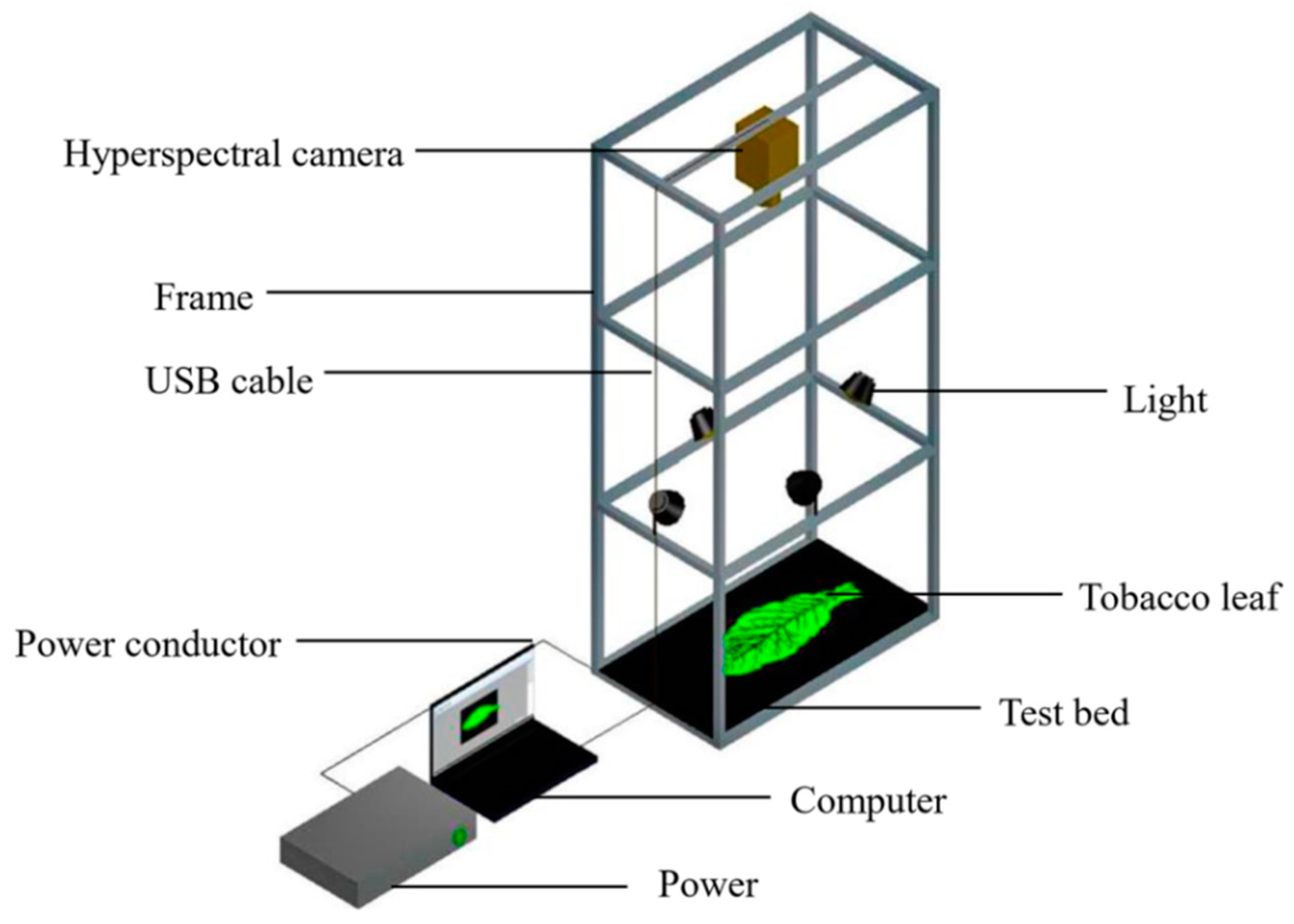
Figure 1. Hyperspectral image acquisition of tobacco leaves.
Processes 11 01249 g001
Figure 2. Principal component analysis images of tobacco leaves at different maturity levels. PC1, PC2, PC3, PC4, and PC5 were the first, second, third, fourth, and fifth principal components.
Processes 11 01249 g002
Figure 3. Original spectral curves of tobacco leaves at different maturity levels.
Processes 11 01249 g003
Figure 4. Spectra obtained with different filtering methods. (A) Baseline, (B) de-trending, (C) MSC, (D) normalize, (E) OSC, (F) SG, (G) SNV, (H) ST, (I) GF, (J) MA, and (K) MF.
Processes 11 01249 g004aProcesses 11 01249 g004b
Figure 5. Characteristic wavelengths of the de-trending spectral curve selected using the SPA.
Processes 11 01249 g005
Figure 6. Characteristic wavelengths of the de-trending spectral curve selected using the PSO algorithm.
Processes 11 01249 g006
Figure 7. Characteristic wavelengths of the de-trending spectral curve selected using the CARS algorithm.
Processes 11 01249 g007
Figure 8. Characteristic wavelengths of the SNV spectral curve selected using the SPA.
Processes 11 01249 g008
Figure 9. Characteristic wavelengths of the SNV spectral curve selected using the PSO algorithm.
Processes 11 01249 g009
Figure 10. Characteristic wavelengths of the SNV spectral curve selected using the CARS algorithm.
Processes 11 01249 g010
Figure 11. Characteristic wavelengths of the MSC spectral curve selected using the SPA.
Processes 11 01249 g011
Figure 12. Characteristic wavelengths of the MSC spectral curve selected using the PSO algorithm.
Processes 11 01249 g012
Figure 13. Characteristic wavelengths of the MSC spectral curve selected using the CARS algorithm.
Processes 11 01249 g013
Table 1. The maturity characteristics of different flue-cured tobacco samples.
Maturity LevelSamples (Piece)Characteristics of Tobacco Leaf
Unripe36The leaves are dark green, the main veins and branches are green, the pubescence is obvious, and the angle between the stalk and leaves is less than 60°.
Under-ripe43The leaves are light green, the main vein is light green, the branch veins are all white, the pubescence is partially shed, and the angle between the stem and leaves is 60°~74°.
Ripe91The leaf surface is light yellow, the main vein and the branch veins are all white, the pubescence fell off, the leaf tip and leaf edge are whitish and rolled down, and the angle between the stem and leaves is 75°~85°.
Over-ripe53The complete leaf surface is yellow, the main veins and branches are white, the pubescence is completely shed, and the angle between the stem and leaves is greater than 85°.
Table 2. Calibration and prediction sets of samples.
Sample SetTotalUnripeUnder-RipeRipeOver-Ripe
Calibration set14825325734
Prediction set6511112419
Table 3. Classification results of PLS-DA for the original and filtered spectra.
Pretreatment MethodPrincipal ComponentsCalibration Set (n = 148)Prediction Set (n = 65)
CorrectAccuracy (%)CorrectAccuracy (%)
Original1413087.84 6092.31
Baseline1212886.49 5584.62
De-trending1913691.896193.85
MSC1614195.276396.92
Normalize1812886.49 5483.08
OSC1510268.92 4569.23
SG1212987.16 5584.62
SNV1313792.576193.85
Spectroscopic1112685.14 5280.00
GF1413087.84 5686.15
MA1312987.16 5686.15
MF1212685.14 5584.62
The data in bold indicate that the classification result is better than the filtering method result of the original spectral data.
Table 4. The results of GA, PLS-DA, LSVM, and BP classification based on characteristic wavelengths.
Filter MethodScreening MethodModelCalibration Set (n = 148)Prediction Set (n = 65)
CorrectAccuracy (%)CorrectAccuracy (%)
De-trendingSPAGA13289.19 5990.77
PLS-DA14094.59 6193.85
LSVM11577.70 5280.00
BPNN11074.32 5076.92
PSOGA11678.38 5076.92
PLS-DA13691.89 5990.77
LSVM10369.59 4772.31
BPNN10872.97 4975.38
CARSGA13691.89 5990.77
PLS-DA13289.19 6092.31
LSVM11678.38 5280.00
BPNN12584.46 5584.62
SNVSPAGA14195.27 6396.92
PLS-DA14799.326498.46
LSVM13893.24 5990.77
BPNN14094.59 6295.38
PSOGA13289.19 5787.69
PLS-DA14396.62 6193.85
LSVM13087.84 5584.62
BPNN13188.51 5686.15
CARSGA12282.43 5381.54
PLS-DA11980.41 5280.00
LSVM13087.84 5990.77
BPNN11879.73 5280.00
MSCSPAGA13792.57 5686.15
PLS-DA14396.62 5990.77
LSVM13591.22 5686.15
BPNN13490.54 5787.69
PSOGA13993.92 5280.00
PLS-DA14597.97 6295.38
LSVM12685.14 5686.15
BPNN12181.76 5584.62
CARSGA12987.16 5889.23
PLS-DA12584.46 5686.15
LSVM10570.95 4772.31
BPNN10872.97 5076.92
The data in bold indicate the best method and the corresponding model performance.
Table 5. Confusion matrices of tobacco leaves with various maturities obtained using SNV-SPA-PLS-DA.
Calibration Set (n = 148)Accuracy (%)Prediction Set (n = 65)Accuracy (%)
UnripeUnder-RipeRipeOver-RipeUnripeUnder-RipeRipeOver-Ripe
Unripe2500010011000100
Under-ripe0320010001100100
Ripe0056010000230100
Over-ripe0013497.140011995
Accuracy/%10010098.2410099.3210010095.8310098.46
Disclaimer/Publisher’s Note: The statements, opinions and data contained in all publications are solely those of the individual author(s) and contributor(s) and not of MDPI and/or the editor(s). MDPI and/or the editor(s) disclaim responsibility for any injury to people or property resulting from any ideas, methods, instructions or products referred to in the content.