Multi-Point Flux MFE Decoupled Method for Compressible Miscible Displacement Problem

Abstract

In this paper, a multi-point flux mixed-finite-element decoupled method was considered for the compressible miscible displacement problem. For this compressible problem, a fully discrete backward Euler scheme was proposed, in which the velocity and pressure equations were decoupled by a multi-point flux MFE method using BDM1 elements combined with a trapezoidal quadrature rule. The concentration equation was handled by a standard FE method. The error analysis for velocity, pressure, and concentration were rigorously derived. Numerical experiments to verify the convergence rates and simulate the miscible displacement problem of a water–oil system were presented.

1. Introduction

In this paper, we considered the miscible displacement of one compressible fluid by another in a porous medium. The $\mathsf{\Omega }\subset R^2$ of unit thickness was described by the following model:

$$\left\{\begin{array}{cc}\hfill & d(c)\frac{\partial p}{\partial t}+\nabla ·\mathbf{u}=q,(x,t)\in \mathsf{\Omega }\times J,\hfill \\ \hfill & \mathbf{u}=-\mu (c)K^{-1}\nabla p,(x,t)\in \mathsf{\Omega }\times J,\hfill \\ \hfill & \varphi \frac{\partial c}{\partial t}+b(c)\frac{\partial p}{\partial t}+\mathbf{u}·\nabla c-\nabla ·(D\nabla c)=(\overline{c}-c)q,(x,t)\in \mathsf{\Omega }\times J,\hfill \end{array}\right.$$

(1)

with the following initial boundary conditions,

$$\left\{\begin{array}{cc}\mathbf{u}·\mathbf{n}=0,\hfill & (x,t)\in \partial \mathsf{\Omega }\times J,\hfill \\ D\nabla c·\mathbf{n}=0,\hfill & (x,t)\in \partial \mathsf{\Omega }\times J,\hfill \\ p(x,0)=p_0(x),\hfill \\ c(x,0)=c_0(x),\hfill \end{array}\right.$$

(2)

where p, $\mathbf{u}$, and c represent the pressure, the Darcy velocity of the fluid, and the concentration of one component in the mixed fluid, respectively; $d(c)$, q, $\mu$, K, and $\varphi$ represent the compression coefficient, external flow rates, the viscosity of the fluid mixture, the permeability tensor, and the porosity of the medium, respectively; $\overline{c}$ is equal to c for production wells and to a specified concentration at injection wells; and in $\mu (c)K^{-1}={\alpha }^{-1}(c)=a(c)$, $J=[0,T]$ is the time interval.

• The diffusion coefficient D was given by:

$$D=\varphi (\mathbf{x})[d_{m}I+|\mathbf{u}|(d_{l}E(\mathbf{u})+d_t{E}^{\perp }(\mathbf{u}))],$$

(3)

where $E(\mathbf{u})={(e_{ij}(\mathbf{u}))}_{2\times 2}$, $e_{ij}(\mathbf{u})=u_i{u}_j/{|\mathbf{u}|}^2$, and $E^{\perp }=I-E,$ $d_m$ are the molecular diffusion coefficients, and $d_l$ and $d_t$ are the longitudinal and transverse dispersion coefficients, respectively.

The past few decades, there has been a significant amount of literature concerning the compressible miscible displacement problem. In [1], the authors presented the Galerkin finite-element procedure and mixed-finite-element procedure to handle the model problem. Bound-preserving discontinuous Galerkin methods were discussed in [2,3,4]. Characteristic block-centered finite-difference method for a compressible miscible displacement problem were derived in [5,6]. In [7,8], the authors presented a mixed-finite-element method with a mass-conservative characteristic finite method to solve a modeled problem. A mixed-finite-element method, combined with a two-grid method, for a compressible miscible displacement problem were shown in [9,10].

The MFE method has been widely used in the simulation of miscible displacement problems because it preserves the local mass and can approximate both the scalar unknown and the negative of its gradient simultaneously, but one limitation of this method has been that it can lead to a saddle-point algebraic system that is time-consuming to solve. To overcome this problem, many scholars have conducted much research on the modification of mixed-finite-element methods. In these works, it has been emphasized that the multi-point flux mixed-finite-element method, as proposed by M.F.Wheeler and I.Yotov [11], not only maintained the advantages of mixed-finite-element methods but also decoupled the saddle-point problem into a symmetric positive definite cell-centered finite-difference scheme for pressure, thereby achieving the rapid decoupling of equations and greatly improving computational efficiency.

There have also been many examples of the application of a multi-point flux mixed-finite-element method. The multi-point flux MFE method for poro-elastic systems on irregular domains with general grids was found in [12]. This method was proposed in [13] for a slightly compressible flow in porous media. The authors in [14] considered a multi-point flux MFE method for a compressible Darcy–Forchheimer model, and it was presented again in [15] for an incompressible Darcy–Forchheimer miscible displacement problem. However, most realistic reservoirs are compressible. Therefore, it was necessary to study rapid decoupling methods for compressible problems. To the best of our knowledge, there has been no published literature demonstrating the multi-point flux MFE method for compressible miscible displacement problems.

Therefore, we adopted a fully discrete backward Euler multi-point flux MFE decoupled scheme for a compressible miscible displacement problem, the velocity–pressure equation was approximated by the multi-point flux MFE method since it was practical for implementation and could decouple the saddle-point algebraic equation into a cell-centered finite difference scheme. In addition, this system was symmetrically positive and definite to achieve fast solutions to the equations, and the concentration equation was approximated by a standard finite element.

In this paper, we used the standard notations of Sobolev norms and spaces, following the example of [16], and we presented the following assumptions on the regularity $(R)$ and the coefficients $(C)$ of (1), which was similar to that in [17], as follows:

$$(R)\left\{\begin{array}{c}p\in L^{\infty }(H^1),\hfill \\ \mathbf{u}\in L^{\infty }(H(div))\cap L^{\infty }(W_{\infty }^1)\cap W_{\infty }^1(L^{\infty })\cap H^2(L^2),\hfill \\ c\in L^{\infty }(H^2)\cap H^1(H^2)\cap L^{\infty }(W_{\infty }^1)\cap H^2(L^2),\hfill \end{array}\right.$$

(4)

$$(C)\left\{\begin{array}{c}{d}_{*}\le d(c)\le d^{*},{\alpha }_{*}\le \alpha (c)\le {\alpha }^{*},{\varphi }_{*}\le \varphi \le {\varphi }^{*},\hfill \\ b_{*}\le b(c)\le b^{*},D_{*}{|\mathbf{r}|}^2\le {\mathbf{r}}^{T}D\mathbf{r}\le D^{*}{|\mathbf{r}|}^2,\forall \mathbf{r}\in R^2,\hfill \\ |\frac{\partial \alpha }{\partial c}(x,c)|+|\frac{\partial d}{\partial c}(x,c)|+|\frac{\partial b}{\partial c}(x,c)|\le \mathcal{K},\hfill \end{array}\right.$$

(5)

where $d_{*},d^{*},{\alpha }_{*},{\alpha }^{*}$, ${\varphi }_{*},{\varphi }^{*}$, $b_{*},b^{*},D_{*},D^{*}$, and $\mathcal{K}$ are positive constants, and throughout the paper, $\mathcal{K}$ could have different values in different scenarios.

The rest of the paper is organized as follows. In Section 2, we present the problem formulation and discretization of the miscible displacement problem. Section 3 is the main body of the paper, where we describe the error-and-convergence analysis for velocity, pressure, and concentration. In Section 4, we illustrate several numerical experiments to demonstrate the theoretical results.

2. Problem Formulation and Discretizations

Assume $\mathsf{\Omega }\in R^2$ was a bounded open domain with the Lipschitz boundary $\partial \mathsf{\Omega }.$ Therefore, let the following be true:

$$\begin{array}{cc}\hfill & H(\mathrm{div},\mathsf{\Omega })=\{\mathbf{u}\in {(L^2(\mathsf{\Omega }))}^2;\nabla ·\mathbf{u}\in L^2(\mathsf{\Omega })\},\hfill \\ \hfill & V=\{\mathbf{u}\in H(\mathrm{div},\mathsf{\Omega });\mathbf{u}·\mathbf{n}=0\},\hfill \\ \hfill & W=L^2(\mathsf{\Omega }),M=H^1(\mathsf{\Omega }).\hfill \end{array}$$

(6)

• Then, we could obtain a weak form of the problem (1): $\forall \omega \in W$, $\mathbf{v}\in V$, $z\in M$, from which we could find $(\mathbf{u},p,c):[0,T]\to (V,W,M)$, as follows:

$$\left\{\begin{array}{c}(d(c)\frac{\partial p}{\partial t},\omega )+(\nabla ·\mathbf{u},\omega )=(q,\omega ),\hfill \\ (\alpha (c)\mathbf{u},\mathbf{v})-(\nabla ·\mathbf{v},p)=0,\hfill \\ (\varphi \frac{\partial c}{\partial t},z)+(b(c)\frac{\partial p}{\partial t},z)+(\mathbf{u}·\nabla c,z)+(D\nabla c,\nabla z)=((\overline{c}-c)q,z).\hfill \end{array}\right.$$

(7)

Assume that $V_h\times W_h$ was the lowest-order Brezzi–Douglas–Marini mixed-finite-element space (${\mathrm{BDM}}_1$) [18]. We considered a quasi-regular quadrilateral partition ${\mathcal{T}}_p$ of $\mathsf{\Omega }$, $h_p=\underset{E\in {\mathcal{T}}_p}{max}\mathrm{diam}(E)$. For each element $E\in {\mathcal{T}}_p$, we defined the bijection mapping $F_E:\overline{E}\to E$, $\overline{E}$ as the reference element with the vertices ${\overline{\mathbf{r}}}_1={(0,0)}^T$, ${\overline{\mathbf{r}}}_2={(1,0)}^T$, ${\overline{\mathbf{r}}}_3={(1,1)}^T$, and ${\overline{\mathbf{r}}}_4={(0,1)}^T$, as well as E with vertices ${\mathbf{r}}_i={(x_i,y_i)}^T$, $i=1,\dots ,4$. For mapping $F_E$, the Jacobian matrix was denoted by $D{F}_E$ and $J_F=|\det (D{F}_E)|$, the inverse mapping by $F_E^{-1}$, and its Jacobian matrix by $D{F}_E^{-1}$ and $J_{F^{-1}}=|\det (D{F}_E^{-1})|$.

For the reference element $\overline{E}$, the ${\mathrm{BDM}}_1$ spaces were defined as follows:

$$\begin{array}{cc}\hfill \overline{V}(\overline{E})& =P_1{(\overline{E})}^2+r\mathrm{curl}({\overline{x}}^2\overline{y})+s\mathrm{curl}(\overline{x}{\overline{y}}^2)\hfill \\ \hfill & =\left(\begin{array}{c}{\alpha }_1\tilde{x}+{\beta }_1\tilde{y}+{\gamma }_1+r{\tilde{x}}^2+2s\tilde{x}\tilde{y}\\ {\alpha }_2\tilde{x}+{\beta }_2\tilde{y}+{\gamma }_2-2r\tilde{x}\tilde{y}-s{\tilde{y}}^2\end{array}\right)\hfill \\ \hfill \overline{W}(\overline{E})& =P_0(\overline{E})=\alpha ,\hfill \end{array}$$

(8)

where ${\alpha }_i$, ${\beta }_i$, ${\gamma }_i$, r, s, and $\alpha$ are the real constants for $i=1,2$.

• In addition, the ${\mathrm{BDM}}_1$ spaces on partition element E were defined by the following transformations:

$$\mathbf{u}\leftrightarrow \overline{\mathbf{u}}:\mathbf{u}=\frac{1}{J_F}D{F}_E\overline{\mathbf{u}}\circ F_E^{-1},vs.\leftrightarrow \overline{v}:v=\overline{v}\circ F_E^{-1}.$$

(9)

• The ${\mathrm{BDM}}_1$ spaces on ${\mathcal{T}}_p$ were given by:

$$\begin{array}{cc}\hfill & V_h=\{\mathbf{v}\in V:\mathbf{v}{|}_E\leftrightarrow \overline{\mathbf{v}},\overline{\mathbf{v}}\in \overline{V}(\overline{E}),\forall E\in {\mathcal{T}}_p\},\hfill \\ \hfill & W_h=\{w\in W:w{|}_E\leftrightarrow \overline{w},\overline{w}\in \overline{W}(\overline{E}),\forall E\in {\mathcal{T}}_p\}.\hfill \end{array}$$

(10)

Let $M_h\subset H^1(\mathsf{\Omega })$ be a standard finite-element space for the Galerkin method with the quasi-regular partition ${\mathcal{T}}_c$ of $\mathsf{\Omega }$, and then, this could satisfy the following:

$$\underset{z_h\in M_h}{\inf }[\parallel z-z_h{\parallel }_{L^2(\mathsf{\Omega })}+h_c\parallel z-z_h{\parallel }_{H^1(\mathsf{\Omega })}]\le \mathcal{K}{h}_c^2{\parallel z\parallel }_{H^2(\mathsf{\Omega })},$$

(11)

where $h_c=\underset{\tau \in {\mathcal{T}}_c}{max}\mathrm{diam}(\tau )$.

• For the approximation spaces, there existed a positive constant $\mathcal{K}$ that was independent of the mesh sizes, such that the following was true:

$${\parallel \mathbf{v}\parallel }_{L^{\infty }}\le \mathcal{K}{h}_p^{-1}{\parallel \mathbf{v}\parallel }_{L^2},\forall \mathbf{v}\in V_h.$$

(12)

$${\parallel z\parallel }_{W^{m,\infty }}\le \mathcal{K}{h}_c^{-1}{\parallel z\parallel }_{H^m},\forall z\in M_h,m=0,1.$$

(13)

• We used the time step, let $N>0$ be a positive integer, and set the following:

$$\Delta t=T/N;t^n=n\Delta t\mathrm{for}n\le T/N.$$

(14)

Next, we considered the global quadrature formula for $\mathbf{u},\mathbf{v}\in V_h$:

$${(\alpha \mathbf{u},\mathbf{v})}_Q=\sum _{E\in {\mathcal{T}}_p}{(\alpha \mathbf{u},\mathbf{v})}_{Q,E},$$

(15)

and the quadrature formula on element E was calculated by mapping the reference element $\overline{E}$:

$$\begin{array}{cc}\hfill {\int }_E\alpha \mathbf{u}·\mathbf{v}\mathrm{d}x& ={\int }_{\overline{E}}\overline{\alpha }\frac{1}{J_F}D{F}_E\overline{\mathbf{u}}·\frac{1}{J_F}D{F}_E\overline{\mathbf{v}}{J}_F\mathrm{d}\overline{x}\doteq {\int }_{\overline{E}}\mathcal{A}\overline{\mathbf{u}}·\overline{\mathbf{v}}\mathrm{d}\overline{x}\hfill \\ \hfill & \equiv \frac{1}{4}\sum _{i=1}^4\mathcal{A}({\overline{\mathbf{r}}}_i)\overline{\mathbf{u}}({\overline{\mathbf{r}}}_i)·\overline{\mathbf{v}}({\overline{\mathbf{r}}}_i),\hfill \end{array}$$

(16)

where

$$\mathcal{A}=\frac{1}{J_F}D{F}_E^T\overline{\alpha }D{F}_E.$$

(17)

• The quadrature error of element E was denoted by the following:

$${\sigma }_E(\alpha \mathbf{u},\mathbf{v})\doteq {(\alpha \mathbf{u},\mathbf{v})}_E-{(\alpha \mathbf{u},\mathbf{v})}_{Q,E},$$

(18)

and the global quadrature error by ${\sigma (\alpha \mathbf{u},\mathbf{v})|}_E={\sigma }_E(\alpha \mathbf{u},\mathbf{v})$.

• In order to avoid a tedious introduction, please refer to [11] for details about the properties of bijection mapping, mixed-element spaces, quadrature formulas, and quadrature errors.

Now, we present the multi-point flux MFE decoupled scheme for the model problem (1), as follows:

$$\left\{\begin{array}{cc}\hfill & (d(c_h^{n-1})\frac{p_h^n-p_h^{n-1}}{\Delta t},{\omega }_h)+(\nabla ·{\mathbf{u}}_h^n,{\omega }_h)=(q^n,{\omega }_h),\forall {\omega }_h\in W_h,\hfill \\ \hfill & {(\alpha (c_h^{n-1}){\mathbf{u}}_h^n,{\mathbf{v}}_h)}_Q-(\nabla ·{\mathbf{v}}_h,p_h^n)=0,\forall {\mathbf{v}}_h\in V_h,\hfill \\ \hfill & (\varphi \frac{c_h^n-c_h^{n-1}}{\Delta t},z_h)+(b(c_h^{n-1})\frac{p_h^n-p_h^{n-1}}{\Delta t},z_h)+({\mathbf{u}}_h^n·\nabla c_h^n,z_h)\hfill \\ \hfill & +(D·\nabla c_h^n,\nabla z_h)=(({\overline{c}}^n-c_h^n)q^n,z_h),\forall z_h\in M_h.\hfill \end{array}\right.$$

(19)

• In order to facilitate the error analysis, we introduced the projection operator.

• For velocity and pressure, we defined projection $(\tilde{\mathbf{u}},\tilde{p})$ such that the following was true:

$$\left\{\begin{array}{ccc}\hfill & (\alpha (c)(\mathbf{u}-\tilde{\mathbf{u}}),{\mathbf{v}}_h)-(p-\tilde{p},\nabla ·{\mathbf{v}}_h)=0,\hfill & \hfill \forall {\mathbf{v}}_h\in V_h,\\ \hfill & (\nabla ·(\mathbf{u}-\tilde{\mathbf{u}}),q_h)=0,\hfill & \hfill \forall q_h\in V_h.\end{array}\right.$$

(20)

• For the following approximation properties,

$$\parallel \mathbf{u}-\tilde{\mathbf{u}}{\parallel \le \mathcal{K}\parallel \mathbf{u}\parallel }_r{h}_p^r,1\le r\le 2,$$

(21)

$$\parallel \nabla ·(\mathbf{u}-\tilde{\mathbf{u}}){\parallel \le \mathcal{K}\parallel \nabla ·\mathbf{u}\parallel }_r{h}_p^r,0\le r\le 1,$$

(22)

$$\parallel p-\tilde{p}{\parallel \le \mathcal{K}\parallel p\parallel }_r{h}_p^r,0\le r\le 1.$$

(23)

• For the concentration, the projection operator $\tilde{c}:J\to M_h$ satisfied:

$$\begin{array}{c}\hfill (D\nabla (\tilde{c}-c),\nabla z)+(\mathbf{u}·\nabla (\tilde{c}-c),z)+(\lambda (\tilde{c}-c),z)=0,z\in M_h,\end{array}$$

(24)

and the approximation properties satisfied:

$$\begin{array}{cc}\hfill & (a)\parallel c-\tilde{c}{\parallel }_{L^{\infty }(L^2(\mathsf{\Omega }))}+h_c\parallel \nabla (c-\tilde{c}){\parallel }_{L^{\infty }(L^2(\mathsf{\Omega }))}\le \mathcal{K}{h}_c^2{\parallel c\parallel }_{L^{\infty }(H^2(\mathsf{\Omega }))},\hfill \\ \hfill & (b)\parallel \frac{\partial (c-\tilde{c})}{\partial t}{\parallel }_{L^{\infty }(L^2(\mathsf{\Omega }))}\le \mathcal{K}{h}_c^2{\{\parallel c\parallel }_{L^{\infty }(H^2(\mathsf{\Omega }))}+\parallel \frac{\partial c}{\partial t}{\parallel }_{L^{\infty }(H^2(\mathsf{\Omega }))}\},\hfill \\ \hfill & (c)\parallel \tilde{c}{\parallel }_{L^{\infty }(W^{1,\infty }(\mathsf{\Omega }))}\le \mathcal{K}.\hfill \end{array}$$

(25)

• For the following convergence analysis, we first introduced specific conclusions, which can be found in [11].

Lemma 1.

There existed a constant $\mathcal{K}$, independent of h, such that for all ${\mathit{v}}_h\in V_h$:

$${(\alpha {\mathit{v}}_h,{\mathit{v}}_h)}_Q\ge \mathcal{K}{\parallel {\mathit{v}}_h\parallel }^2.$$

(26)

Remark 1.

Lemma 1 implied that ${(\alpha ·,·)}_Q^{1/2}$ is a norm. We denoted this norm by ${\parallel ·\parallel }_Q$. It was easy to observe that ${\parallel ·\parallel }_Q$ was equivalent to $\parallel ·\parallel$.

Lemma 2.

There existed a constant $\mathcal{K}$, independent of h and $\Delta t$, such that for all ${\mathit{v}}_h\in V_h$, the following was true:

$$|\sigma (\alpha \tilde{\mathit{u}},{\mathit{v}}_h){|\le \mathcal{K}h\parallel \mathit{u}\parallel }_1\parallel {\mathit{v}}_h\parallel .$$

(27)

3. Convergence Analysis

Note the following: $\eta =p-\tilde{p},\theta =\tilde{p}-p_h,\mathbf{\gamma }=\mathbf{u}-\tilde{\mathbf{u}},\mathbf{\delta }=\tilde{\mathbf{u}}-{\mathbf{u}}_h$,$\zeta =c-\tilde{c},\xi =\tilde{c}-c_h,d_t{\theta }^n=\frac{{\theta }^n-{\theta }^{n-1}}{\Delta t},d_t{\mathbf{\delta }}^n=\frac{{\mathbf{\delta }}^n-{\mathbf{\delta }}^{n-1}}{\Delta t}$.

Theorem 1.

There existed a constant $\mathcal{K}$, independent of h and $\Delta t$, such that the following was true:

$$\begin{array}{cc}\hfill \parallel d_t{\theta }^N{\parallel }^2+\Delta t\sum _{n=1}^N{\parallel d_t{\mathbf{\delta }}^n\parallel }^2& \le \mathcal{K}(\Delta t^2+h_p^2+h_c^4+\Delta t\sum _{n=1}^N(\parallel d_t{\xi }^{n-1}{\parallel }^2+\parallel {\mathbf{\delta }}^{n-1}{\parallel }^2)).\hfill \end{array}$$

(28)

Proof. 

Subtracting the first two formulas of the multi-point flux MFE scheme (19) from the first two formulas of variational formulation (7) and combing that with the projection operator (20), we could express the error equations, as follows:

$$\left\{\begin{array}{cc}\hfill & (d(c_h^{n-1})\frac{{\theta }^n-{\theta }^{n-1}}{\Delta t},{\omega }_h)+(\nabla ·{\mathbf{\delta }}^n,{\omega }_h)=-(d(c_h^{n-1})\frac{{\eta }^n-{\eta }^{n-1}}{\Delta t},{\omega }_h)\hfill \\ \hfill & -(d(c_h^{n-1})(\frac{\partial p^n}{\partial t}-\frac{p^n-p^{n-1}}{\Delta t}),{\omega }_h)-(d(c^n)\frac{\partial p^n}{\partial t}-d(c_h^{n-1})\frac{\partial p^n}{\partial t},{\omega }_h),\hfill \\ \hfill & {(\alpha (c_h^{n-1}){\mathbf{\delta }}^n,{\mathbf{v}}_h)}_Q-({\theta }^n,\nabla ·{\mathbf{v}}_h)=-((\alpha (c^n)-\alpha (c_h^{n-1})){\tilde{\mathbf{u}}}^n,{\mathbf{v}}_h)\hfill \\ \hfill & -\sigma (\alpha (c_h^{n-1}){\tilde{\mathbf{u}}}^n,{\mathbf{v}}_h).\hfill \end{array}\right.$$

(29)

• Subtracting the n time level and $n-1$ time level of the error equation, dividing that by $\Delta t$, and then taking ${\omega }_h=d_t{\theta }^n$ and ${\mathbf{v}}_h=d_t{\mathbf{\delta }}^n$, as well as adding in the two formulas, we could deduce the following:

$$\begin{array}{cc}\hfill & (d_t(d(c_h^{n-1})d_t{\theta }^n),d_t{\theta }^n)+{(d_t(\alpha (c_h^{n-1}){\mathbf{\delta }}^n),d_t{\mathbf{\delta }}^n)}_Q\hfill \\ & =(d_t((\alpha (c_h^{n-1})-\alpha (c^n)){\tilde{\mathbf{u}}}^n),d_t{\mathbf{\delta }}^n)-\sigma (d_t(\alpha (c_h^{n-1}){\tilde{\mathbf{u}}}^n),d_t{\mathbf{\delta }}^n)\hfill \\ & -(d_t((d(c^n)-d(c_h^{n-1}))\frac{\partial p^n}{\partial t}),d_t{\theta }^n)\hfill \\ & -(d_t(d(c_h^{n-1})(\frac{\partial p^n}{\partial t}-\frac{p^n-p^{n-1}}{\Delta t})),d_t{\theta }^n)-(d_t(d(c_h^{n-1})d_t{\eta }^n),d_t{\theta }^n).\hfill \end{array}$$

(30)

• Based on the following:

$$\begin{array}{cc}\hfill & (d_t(d(c_h^{n-1})d_t{\theta }^n),d_t{\theta }^n)\ge \frac{1}{2}{d}_t(d(c_h^{n-1})d_t{\theta }^n,d_t{\theta }^n)\hfill \\ & -\frac{1}{2}(d_t(d(c_h^{n-1}))d_t{\theta }^{n-1},d_t{\theta }^{n-1})+(d_t(d(c_h^{n-1}))d_t{\theta }^{n-1},d_t{\theta }^n),\hfill \end{array}$$

(31)

and

$${(d_t(\alpha (c_h^{n-1}){\mathbf{\delta }}^n),d_t{\mathbf{\delta }}^n)}_Q={(\alpha (c_h^{n-1})d_t{\mathbf{\delta }}^n,d_t{\mathbf{\delta }}^n)}_Q+{(d_t(\alpha (c_h^{n-1})){\mathbf{\delta }}^{n-1},d_t{\mathbf{\delta }}^n)}_Q.$$

• We concluded:

$$\begin{array}{cc}\hfill & {(\alpha (c_h^{n-1})d_t{\mathbf{\delta }}^n,d_t{\mathbf{\delta }}^n)}_Q+\frac{1}{2}{d}_t(d(c_h^{n-1})d_t{\theta }^n,d_t{\theta }^n)\le -{(d_t(\alpha (c_h^{n-1})){\mathbf{\delta }}^{n-1},d_t{\mathbf{\delta }}^n)}_Q\hfill \\ & -(d_t(d(c_h^{n-1}))d_t{\theta }^{n-1},d_t{\theta }^n)+\frac{1}{2}(d_t(d(c_h^{n-1}))d_t{\theta }^{n-1},d_t{\theta }^{n-1})\hfill \\ & +(d_t((\alpha (c_h^{n-1})-\alpha (c^n)){\tilde{\mathbf{u}}}^n),d_t{\mathbf{\delta }}^n)-\sigma (d_t(\alpha (c_h^{n-1}){\tilde{\mathbf{u}}}^n),d_t{\mathbf{\delta }}^n)\hfill \\ & -(d_t((d(c^n)-d(c_h^{n-1}))\frac{\partial p^n}{\partial t}),d_t{\theta }^n)-(d_t(d(c_h^{n-1})(\frac{\partial p^n}{\partial t}-\frac{p^n-p^{n-1}}{\Delta t})),d_t{\theta }^n)\hfill \\ & -(d_t(d(c_h^{n-1})d_t{\eta }^n),d_t{\theta }^n).\hfill \end{array}$$

• Multiplying the above formula by $\Delta t$ and then combining Lemma 1 and summing n from 1 to N, we could then obtain the following:

$$\begin{array}{cc}\hfill C& \Delta t\sum _{n=1}^N\parallel d_t{\mathbf{\delta }}^n{\parallel }_{L^2}^2+{\parallel d_t{\theta }^N\parallel }_{L^2}^2\le -\sum _{n=1}^N\Delta t{(d_t(\alpha (c_h^{n-1})){\mathbf{\delta }}^{n-1},d_t{\mathbf{\delta }}^n)}_Q\hfill \\ & -\sum _{n=1}^N\Delta t(d_t(d(c_h^{n-1}))d_t{\theta }^{n-1},d_t{\theta }^n)+\frac{1}{2}\sum _{n=1}^N\Delta t(d_t(d(c_h^{n-1}))d_t{\theta }^{n-1},d_t{\theta }^{n-1})\hfill \\ & +\sum _{n=1}^N\Delta t(d_t((\alpha (c_h^{n-1})-\alpha (c^n)){\tilde{\mathbf{u}}}^n),d_t{\mathbf{\delta }}^n)-\sum _{n=1}^N\Delta t\sigma (d_t(\alpha (c_h^{n-1}){\tilde{\mathbf{u}}}^n),d_t{\mathbf{\delta }}^n)\hfill \\ & -\sum _{n=1}^N\Delta t(d_t((d(c^n)-d(c_h^{n-1}))\frac{\partial p^n}{\partial t}),d_t{\theta }^n)\hfill \\ & -\sum _{n=1}^N\Delta t(d_t(d(c_h^{n-1})(\frac{\partial p^n}{\partial t}-\frac{p^n-p^{n-1}}{\Delta t})),d_t{\theta }^n)\hfill \\ & -\sum _{n=1}^N\Delta t(d_t(d(c_h^{n-1})d_t{\eta }^n),d_t{\theta }^n)\hfill \\ \hfill =& \sum _{n=1}^8{T}_i.\hfill \end{array}$$

(32)

• Next, we estimate the Formula (32), item by item:

$$\begin{array}{cc}\hfill |T_1|& =|\Delta t\sum _{n=1}^N{(d_t(\alpha (c_h^{n-1})){\mathbf{\delta }}^{n-1},d_t{\mathbf{\delta }}^n)}_Q|\hfill \\ & \le \epsilon \Delta t\sum _{n=1}^N\parallel d_t{\mathbf{\delta }}^n{\parallel }_{L^2}^2+\mathcal{K}\Delta t\sum _{n=1}^N(1+\parallel d_t{\xi }^{n-1}{\parallel }_{L^{\infty }}^2+h_c^4)\parallel {\mathbf{\delta }}^{n-1}{\parallel }_{L^2}^2,\hfill \end{array}$$

(33)

which follows the properties (5), Remark 1, and the $\epsilon$-inequality.

$$\begin{array}{cc}\hfill |T_2|+|T_3|=& |\Delta t\sum _{n=1}^N(d_t(d(c_h^{n-1}))d_t{\theta }^{n-1},d_t{\theta }^n)|\hfill \\ \hfill & +\frac{1}{2}|\Delta t\sum _{n=1}^N(d_t(d(c_h^{n-1}))d_t{\theta }^{n-1},d_t{\theta }^{n-1})|\hfill \\ \hfill \le & \mathcal{K}\Delta t\sum _{n=1}^N(1+\parallel d_t{\xi }^{n-1}{\parallel }_{L^{\infty }}^2)\parallel d_t{\theta }^{n-1}{\parallel }_{L^2}^2+\mathcal{K}\Delta t\sum _{n=1}^N{\parallel d_t{\theta }^n\parallel }_{L^2}^2.\hfill \end{array}$$

(34)

$$\begin{array}{cc}\hfill |T_4|& =|\Delta t\sum _{n=1}^N(d_t((\alpha (c_h^{n-1})-\alpha (c^n)){\tilde{\mathbf{u}}}^n),d_t{\mathbf{\delta }}^n)|\hfill \\ & \le \epsilon \Delta t\sum _{n=1}^N\parallel d_t{\mathbf{\delta }}^n{\parallel }_{L^2}^2+\mathcal{K}(\Delta t\sum _{n=1}^N\parallel d_t{\xi }^{n-1}{\parallel }_{L^2}^2+\Delta t^2+h_c^4).\hfill \end{array}$$

(35)

$$\begin{array}{cc}\hfill |T_5|& =|\Delta t\sum _{n=1}^N\sigma (d_t(\alpha (c_h^{n-1}){\tilde{\mathbf{u}}}^n),d_t{\mathbf{\delta }}^n)|\hfill \\ \hfill & =|\Delta t\sum _{n=1}^N\sigma (\alpha (c_h^{n-1})d_t{\tilde{\mathbf{u}}}^n+d_t(\alpha (c_h^{n-1})){\tilde{\mathbf{u}}}^{n-1},d_t{\mathbf{\delta }}^n)|\hfill \\ \hfill & \le \epsilon \Delta t\sum _{n=1}^N{\parallel d_t{\mathbf{\delta }}^n\parallel }_{L^2}^2+\mathcal{K}{h}_p^2,\hfill \end{array}$$

(36)

which followed Lemma 2 and the $\epsilon$-inequality.

$$\begin{array}{cc}\hfill |T_6|& =|\Delta t\sum _{n=1}^N(d_t((d(c^n)-d(c_h^{n-1}))\frac{\partial p^n}{\partial t}),d_t{\theta }^n)|\hfill \\ & \le \mathcal{K}(\Delta t\sum _{n=1}^N(\parallel d_t{\theta }^n{\parallel }_{L^2}^2+\parallel d_t{\xi }^{n-1}{\parallel }_{L^2}^2)+\Delta t^2+h_c^4).\hfill \end{array}$$

(37)

$$\begin{array}{cc}\hfill |T_7|+|T_8|\le & |\Delta t\sum _{n=1}^N(d_t(d(c_h^{n-1})(\frac{\partial p^n}{\partial t}-\frac{p^n-p^{n-1}}{\Delta t})),d_t{\theta }^n)|\hfill \\ & +|\Delta t\sum _{n=1}^N(d_t(d(c_h^{n-1})d_t{\eta }^n),d_t{\theta }^n)|\hfill \\ \hfill \le & \mathcal{K}(\Delta t\sum _{n=1}^N(\parallel d_t{\theta }^n{\parallel }_{L^2}^2+\parallel d_t{\xi }^{n-1}{\parallel }_{L^{\infty }}^2)+\Delta t^2+h_p^2+h_c^4).\hfill \end{array}$$

(38)

• Substituting (33)–(38) into (32), and combining the discrete Gronwall’s inequality, we obtained (28), which completed the proof of the theorem. □

Theorem 2.

Assume that (4), (5), and (11)–(13) held. The discretization parameters obeyed the relationship $\Delta t=O(h_p)$, $h_c^2=O(h_p)$. Then, there exists a positive constant $\mathcal{K}$, independent of h and $\Delta t$, such that the following was true:

$$\Delta t\sum _{n=1}^N\parallel d_t{\xi }^n{\parallel }^2+\parallel \nabla {\xi }^N{\parallel }^2\le \mathcal{K}(\Delta t^2+h_p^2+h_c^4+\Delta t\sum _{n=1}^N(\parallel {\xi }^n{\parallel }_1^2+\parallel d_t{\theta }^n{\parallel }^2)).$$

(39)

Proof. 

Subtracting the last formula of the approximation scheme (19) from the last formula of the variational formulation (7), and then integrating the projection operator (24) yielded the following error equation:

$$\begin{array}{cc}\hfill & (\varphi \frac{{\xi }^n-{\xi }^{n-1}}{\Delta t},z_h)+(D·\nabla {\xi }^n,\nabla z_h)=-(\varphi (\frac{\partial c^n}{\partial t}-\frac{c^n-c^{n-1}}{\Delta t}),z_h)\hfill \\ & -(\varphi \frac{{\zeta }^n-{\zeta }^{n-1}}{\Delta t},z_h)+(b(c_h^{n-1})\frac{p_h^n-p_h^{n-1}}{\Delta t},z_h)-(b(c^n)\frac{\partial p^n}{\partial t},z_h)\hfill \\ & -({\mathbf{u}}^n·\nabla {\tilde{c}}^n-{\mathbf{u}}_h^n·\nabla c_n^n,z_h)+((c_h^n-c^n)q^n,z_h)+(\lambda {\zeta }^n,z_h).\hfill \end{array}$$

(40)

• Taking $z_h=d_t{\xi }^n$ and multiplying $\Delta t$ on both sides of (40), and then summing for n from 1 to N, we obtained the following:

$$\begin{array}{cc}\hfill & \Delta t\sum _{n=1}^N(\varphi d_t{\xi }^n,d_t{\xi }^n)+\Delta t\sum _{n=1}^N(D·\nabla {\xi }^n,\nabla d_t{\xi }^n)\hfill \\ \hfill =& -\Delta t\sum _{n=1}^N(\varphi (\frac{\partial c}{\partial t}-\frac{c^n-c^{n-1}}{\Delta t}),d_t{\xi }^n)-\Delta t\sum _{n=1}^N(\varphi \frac{{\zeta }^n-{\zeta }^{n-1}}{\Delta t},d_t{\xi }^n)\hfill \\ & +\Delta t\sum _{n=1}^N(b(c_h^{n-1})\frac{p_h^n-p_h^{n-1}}{\Delta t},d_t{\xi }^n)-\Delta t\sum _{n=1}^N(b(c^n)\frac{\partial p^n}{\partial t},d_t{\xi }^n)\hfill \\ \hfill & -\Delta t\sum _{n=1}^N({\mathbf{u}}^n·\nabla {\tilde{c}}^n-{\mathbf{u}}_h^n·\nabla c_n^n,d_t{\xi }^n)+\Delta \sum _{n=1}^N((c_h^n-c^n)q^n,d_t{\xi }^n)\hfill \\ \hfill & +\Delta t\sum _{n=1}^N(\lambda {\zeta }^n,d_t{\xi }^n)\doteq \sum _{n=1}^7{I}_i.\hfill \end{array}$$

(41)

• The left side of the previous equation could be estimated as follows:

$$\begin{array}{cc}\hfill \Delta t\sum _{n=1}^N(\varphi d_t{\xi }^n,d_t{\xi }^n)& +\Delta t\sum _{n=1}^N(D·\nabla {\xi }^n,\nabla d_t{\xi }^n)\ge \mathcal{K}\Delta t\sum _{n=1}^N{\parallel d_t{\xi }^n\parallel }^2\hfill \\ \hfill & +\frac{1}{2\Delta t}(D·\nabla {\xi }^n,\nabla {\xi }^n)-\frac{1}{2\Delta t}(D·\nabla {\xi }^{n-1},\nabla {\xi }^{n-1}).\hfill \end{array}$$

(42)

• We estimated the right side of Formula (41) using the Cauchy–Schwarz inequality, and we obtained the following:

$$\begin{array}{cc}\hfill |I_1|& =|\Delta t\sum _{n=1}^N(\varphi (\frac{\partial c}{\partial t}-\frac{c^n-c^{n-1}}{\Delta t}),d_t{\xi }^n)|\hfill \\ \hfill & \le \Delta t\sum _{n=1}^N(\mathcal{K}\parallel \varphi \frac{c^n-c^{n-1}}{\Delta t}-\varphi \frac{\partial c}{\partial t}{\parallel }_{L^2}^2+\epsilon \parallel d_t{\xi }^n{\parallel }_{L^2}^2)\hfill \\ \hfill & \le \mathcal{K}\Delta t\sum _{n=1}^N\parallel {\int }_{t^{n-1}}^{t^n}\frac{{\partial }^{2}c}{\partial t^2}{dt\parallel }_{L^2}^2+\epsilon \Delta t\sum _{n=1}^N{\parallel d_t{\xi }^n\parallel }_{L^2}^2\hfill \\ \hfill & \le \mathcal{K}\Delta t^2\parallel \frac{{\partial }^{2}c}{\partial t^2}{\parallel }_{L^2(0,T;L^2)}^2+\epsilon \Delta t\sum _{n=1}^N{\parallel d_t{\xi }^n\parallel }_{L^2}^2.\hfill \end{array}$$

(43)

$$\begin{array}{cc}\hfill |I_2|& =|\Delta t\sum _{n=1}^N(\varphi \frac{{\zeta }^n-{\zeta }^{n-1}}{\Delta t},d_t{\xi }^n)|\hfill \\ \hfill & \le \Delta t\sum _{n=1}^N\mathcal{K}{\left[{\int }_{\mathsf{\Omega }}{({\int }_{t^{n-1}}^{t^n}\frac{\partial \zeta }{\partial t}dt)}^{2}dx\right]}^{\frac{1}{2}}·{\left[{\int }_{\mathsf{\Omega }}{(d_t{\xi }^n)}^{2}dx\right]}^{\frac{1}{2}}\hfill \\ \hfill & \le \mathcal{K}\Delta t\sum _{n=1}^N{\left[{\int }_{\mathsf{\Omega }}({\int }_{t^{n-1}}^{t^n}{1}^{2}dt{\int }_{t^{n-1}}^{t^n}{(\frac{\partial \zeta }{\partial t})}^{2}dt)dx\right]}^{\frac{1}{2}}·{\parallel d_t{\xi }^n\parallel }_{L^2}\hfill \\ \hfill & \le \mathcal{K}\sum _{n=1}^N\parallel \frac{\partial \zeta }{\partial t}{\parallel }_{L^2(t^{n-1},t^n;L^2)}^2+\epsilon \sum _{n=1}^N\Delta t{\parallel d_t{\xi }^n\parallel }_{L^2}^2\hfill \\ \hfill & \le \mathcal{K}{h}_c^4\parallel \frac{\partial c}{\partial t}{\parallel }_{L^2(0,T;H^2)}^2+\epsilon \Delta t\sum _{n=1}^N{\parallel d_t{\xi }^n\parallel }_{L^2}^2.\hfill \end{array}$$

(44)

$$\begin{array}{cc}\hfill |I_3+I_4|=& |\Delta t\sum _{n=1}^N(b(c_h^{n-1})\frac{p_h^n-p_h^{n-1}}{\Delta t},d_t{\xi }^n)-\Delta t\sum _{n=1}^N(b(c^n)\frac{\partial p^n}{\partial t},d_t{\xi }^n)|\hfill \\ \hfill =& |\Delta t\sum _{n=1}^N((b(c_h^{n-1})(\frac{p_h^n-p_h^{n-1}}{\Delta t}-\frac{p^n-p^{n-1}}{\Delta t}),d_t{\xi }^n)\hfill \\ \hfill & +(b(c_h^{n-1})(\frac{p^n-p^{n-1}}{\Delta t}-\frac{\partial p^n}{\partial t}),d_t{\xi }^n)+((b(c_h^{n-1})-b(c^n))\frac{\partial p^n}{\partial t},d_t{\xi }^n))|\hfill \\ \hfill \le & \mathcal{K}(\Delta t^2+h_p^2+h_c^4+\Delta t\sum _{n=1}^N(\parallel {\xi }^{n-1}{\parallel }_{L^2}^2+\parallel d_t{\theta }^n{\parallel }_{L^2}^2))+\epsilon \Delta t\sum _{n=1}^N{\parallel d_t{\xi }^n\parallel }_{L^2}^2.\hfill \end{array}$$

(45)

$$\begin{array}{cc}\hfill |I_5|=& |\Delta t\sum _{n=1}^N({\mathbf{u}}^n·\nabla {\tilde{c}}^n-{\mathbf{u}}_h^n·\nabla c_n^n,d_t{\xi }^n)|\hfill \\ \hfill \le & |\Delta t\sum _{n=1}^N(({\mathbf{u}}^n-{\mathbf{u}}_h^n)·\nabla {\tilde{c}}^n,d_t{\xi }^n)|+|\Delta t\sum _{n=1}^N({\mathbf{u}}_h^n·\nabla ({\tilde{c}}^n-c_h^n),d_t{\xi }^n)|\hfill \\ \hfill \le & \Delta t\sum _{n=1}^N|(a(c^n)\nabla p^n-a(c_h^n)\nabla p_h^n)·\nabla {\tilde{c}}^n,d_t{\xi }^n)|\hfill \\ \hfill & +\Delta t\sum _{n=1}^N\parallel {\mathbf{u}}_h^n{\parallel }_{L^{\infty }}\parallel \nabla ({\tilde{c}}^n-c_h^n){\parallel }_{L^2}{\parallel d_t{\xi }^n\parallel }_{L^2}\hfill \\ \hfill =& \Delta t\sum _{n=1}^N|((a(c^n)-a(c_h^n))\nabla p_h^n·\nabla {\tilde{c}}^n,d_t{\xi }^n)+(a(c^n)\nabla {\theta }^n·\nabla {\tilde{c}}^n,d_t{\xi }^n)\hfill \\ \hfill & +(a(c^n)\nabla {\eta }^n·\nabla {\tilde{c}}^n,d_t{\xi }^n)|+\Delta t\sum _{n=1}^N\parallel {\mathbf{u}}_h^n{\parallel }_{L^{\infty }}\parallel \nabla ({\tilde{c}}^n-c_h^n){\parallel }_{L^2}{\parallel d_t{\xi }^n\parallel }_{L^2}\hfill \\ \hfill \le & \mathcal{K}(h_p^2+h_c^4+\Delta t\sum _{n=1}^N\parallel {\xi }^n{\parallel }_1^2)+\epsilon \Delta t\sum _{n=1}^N{\parallel d_t{\xi }^n\parallel }_{L^2}^2.\hfill \end{array}$$

(46)

• The estimation technique of (46) was similar to Formula $(3.22)$ in [1]. The constant $\mathcal{K}$ in (46) depended on the norms of $\parallel \nabla p_h^n{\parallel }_{L^{\infty }}$, $\parallel {\mathbf{u}}_h^n{\parallel }_{L^{\infty }}$ and $\parallel \nabla {\theta }^n{\parallel }_{L^{\infty }}$, such that they could be bounded using the inductive hypothesis, which we did not elaborate here.

$$\begin{array}{cc}\hfill |I_6|& =|\Delta t\sum _{n=1}^N((c_h^n-c^n)q^n,d_t{\xi }^n)|\hfill \\ \hfill & \le \mathcal{K}{h}_c^4+\mathcal{K}\Delta t\sum _{n=1}^N\parallel {\xi }^n{\parallel }_{L^2}^2+\epsilon \Delta t\sum _{n=1}^N{\parallel d_t{\xi }^n\parallel }_{L^2}^2,\hfill \end{array}$$

(47)

follows from (25a) and the Cauchy–Schwarz inequality. We could also obtain the following:

$$|I_7|=|\Delta t\sum _{n=1}^N(\lambda {\zeta }^n,d_t{\xi }^n)|\le \mathcal{K}{h}_c^4+\epsilon \Delta t\sum _{n=1}^N{\parallel d_t{\xi }^n\parallel }_{L^2}^2.$$

(48)

• Substituting (42)–(48) into (41), choosing ${\xi }^0=0$, and applying the discrete Gronwall’s Lemma, we discovered the following:

$$\Delta t\sum _{n=1}^N\parallel d_t{\xi }^n{\parallel }^2+\parallel \nabla {\xi }^N{\parallel }^2\le \mathcal{K}(\Delta t^2+h_p^2+h_c^4+\Delta t\sum _{n=1}^N(\parallel {\xi }^n{\parallel }_1^2+\parallel d_t{\theta }^n{\parallel }^2)),$$

(49)

this completes the proof of Theorem 2. □

Moreover, by observing the following:

$$\begin{array}{cc}\hfill \Delta t\sum _{n=1}^N({\phi }^n,d_t{\phi }^n)& =\frac{1}{2}(\parallel {\phi }^N{\parallel }^2-\parallel {\phi }^0{\parallel }^2+\sum _{n=1}^N\parallel {\phi }^n-{\phi }^{n-1}{\parallel }^2)\hfill \\ \hfill & \le \frac{1}{2\epsilon }\Delta t\sum _{n=1}^N({\phi }^n,{\phi }^n)+\frac{\epsilon }{2}\Delta t\sum _{n=1}^N(d_t{\phi }^n,d_t{\phi }^n),\hfill \end{array}$$

(50)

it followed that:

$$\begin{array}{cc}\hfill & \parallel {\phi }^N{\parallel }^2-\parallel {\phi }^0{\parallel }^2\le \mathcal{K}\Delta t\sum _{n=1}^N\parallel {\phi }^n{\parallel }^2+\epsilon \Delta t\sum _{n=1}^N{\parallel d_t{\phi }^n\parallel }^2.\hfill \end{array}$$

(51)

• Then, combing (28) and (39), we obtained the following:

$$\begin{array}{cc}\hfill & \parallel {\theta }^N{\parallel }^2+\parallel d_t{\theta }^N{\parallel }^2+\parallel {\mathbf{\delta }}^N{\parallel }^2+\Delta t\sum _{n=1}^N\parallel d_t{\mathbf{\delta }}^n{\parallel }^2+\parallel \nabla {\xi }^N{\parallel }^2+\parallel {\xi }^N{\parallel }^2+\Delta t\sum _{n=1}^N{\parallel d_t{\xi }^n\parallel }^2\hfill \\ & \le \mathcal{K}\Delta t\sum _{n=1}^N(\parallel {\theta }^n{\parallel }^2+\parallel {\mathbf{\delta }}^n{\parallel }^2+\parallel {\xi }^n{\parallel }_1^2+\parallel d_t{\theta }^n{\parallel }^2)+\mathcal{K}(\Delta t^2+h_c^4+h_p^2).\hfill \end{array}$$

(52)

• Applying the discrete Gronwall’s Lemma to the previous equation resulted in the following:

$$\begin{array}{cc}\hfill & \underset{n=1}{\overset{N}{max}}\parallel {\theta }^N{\parallel }^2+\underset{n=1}{\overset{N}{max}}\parallel {\mathbf{\delta }}^N{\parallel }^2+\underset{n=1}{\overset{N}{max}}\parallel {\xi }^N{\parallel }^2+\underset{n=1}{\overset{N}{max}}\parallel \nabla {\xi }^N{\parallel }^2+\underset{n=1}{\overset{N}{max}}{\parallel d_t{\theta }^N\parallel }^2\hfill \\ & +\Delta t\sum _{n=1}^N\parallel d_t{\mathbf{\delta }}^n{\parallel }^2+\Delta t\sum _{n=1}^N{\parallel d_t{\xi }^n\parallel }^2\le \mathcal{K}(h_c^4+h_p^2+\Delta t^2).\hfill \end{array}$$

(53)

• Combining the estimates (21), (23), (25), and (53), we obtained the following conclusion.

Corollary 1.

Under the assumption of Theorem 2, there existed a constant $\mathcal{K}$, independent of h and $\Delta t$, such that the following was true:

$$\begin{array}{c}\hfill \underset{n=1}{\overset{N}{max}}\parallel {\mathit{u}}^n-{\mathit{u}}_h^n\parallel +\underset{n=1}{\overset{N}{max}}\parallel p^n-p_h^n\parallel +\underset{n=1}{\overset{N}{max}}\parallel c^n-c_h^n\parallel \le \mathcal{K}(\Delta t+h_c^2+h_p).\end{array}$$

(54)

4. Numerical Examples

In this section, we present the numerical experiments that verified the theoretical analysis and tested the performance of the proposed method.

4.1. Test Convergence Rate

We considered the problem (1) in $\mathsf{\Omega }=[0,1]\times [0,1]$ and $K=1$. The exact solution was constructed as follows:

$$\begin{array}{cc}\hfill & \mathbf{u}(x,y,t)=-exp(t)(sin(\pi x)cos(\pi y)+3x^2{y}^2,cos(\pi x)sin(\pi y)+2x^{3}y),\hfill \\ \hfill & p(x,y,t)=exp(t)(-cos(\pi x)cos(\pi y)/\pi +x^3{y}^2),\hfill \\ \hfill & c(x,y,t)=exp(t)(sin(\pi x)+sin(\pi y)).\hfill \end{array}$$

The numerical results in

Table 1. Numerical error-and-convergence rates for Example $4.1$.

Norm Type	$\parallel \mathbf{u}-{\mathbf{u}}_h{\parallel }_{l^2(L^2)}$		$\parallel \mathbf{u}-{\mathbf{u}}_h{\parallel }_{l^{\infty }(L^2)}$		$\parallel p-p_h{\parallel }_{l^2(L^2)}$		$\parallel p-p_h{\parallel }_{l^{\infty }(L^2)}$
mesh	error	rate	error	rate	error	rate	error	rate
5	$4.15\times {10}^{-3}$	—	$1.31\times {10}^{-1}$	—	$1.37\times {10}^{-3}$	—	$4.32\times {10}^{-2}$	—
10	$1.97\times {10}^{-3}$	1.01	$6.23\times {10}^{-2}$	1.01	$6.97\times {10}^{-4}$	0.97	$2.21\times {10}^{-2}$	0.97
20	$9.99\times {10}^{-4}$	0.98	$3.16\times {10}^{-2}$	0.98	$3.50\times {10}^{-4}$	0.99	$1.11\times {10}^{-2}$	0.99
40	$5.08\times {10}^{-4}$	0.98	$1.61\times {10}^{-2}$	0.98	$1.55\times {10}^{-4}$	1.00	$5.55\times {10}^{-3}$	1.00
Norm Type	$\parallel c-c_h{\parallel }_{l^2(H^1)}$		$\parallel c-c_h{\parallel }_{l^{\infty }(H^1)}$		$\parallel c-c_h{\parallel }_{l^2(L^2)}$		$\parallel c-c_h{\parallel }_{l^{\infty }(L^2)}$
mesh	error	rate	error	rate	error	rate	error	rate
5	$1.80\times {10}^{-2}$	—	$5.68\times {10}^{-1}$	—	$2.94\times {10}^{-4}$	—	$4.65\times {10}^{-2}$	—
10	$9.00\times {10}^{-3}$	1.00	$2.85\times {10}^{-1}$	0.99	$7.37\times {10}^{-5}$	1.97	$1.17\times {10}^{-2}$	1.99
20	$4.50\times {10}^{-3}$	1.00	$1.42\times {10}^{-1}$	1.00	$1.84\times {10}^{-5}$	1.99	$2.92\times {10}^{-3}$	2.00
40	$2.25\times {10}^{-3}$	1.00	$7.12\times {10}^{-2}$	1.00	$4.61\times {10}^{-6}$	2.00	$7.29\times {10}^{-4}$	2.00

show the first-order convergence rates for velocity and pressure. Moreover, the first-order convergence rates of the $H^1$ norms and the second-order rates of the $L^2$ norms for concentration were consistent with the theoretical analysis.The graphs of the concentration, pressure, and velocity fields are presented in Figure 1.

We tested the application performance of the proposed method for different injection production cases of water–oil miscible displacements.

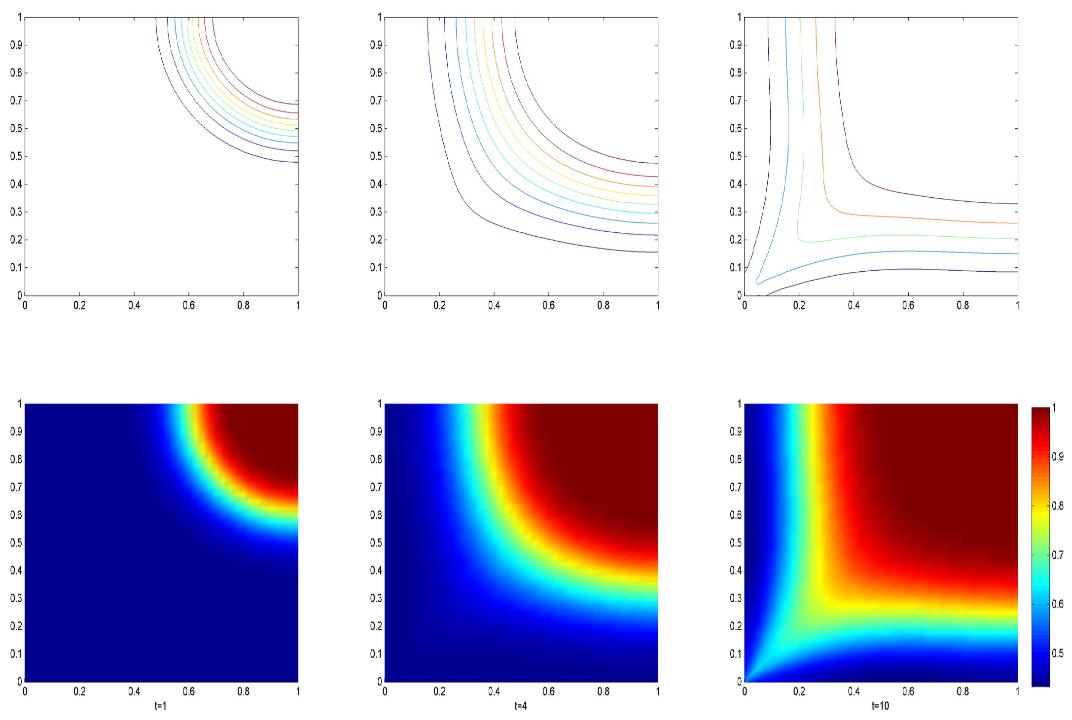
4.2. Single Injection Single Production Case

For the single-injection, single-production case, $K=0.01$, we set the injection well in the upper-right corner at $q=20$ and m${}^2$/s, and the production well in lower-right corner at $q=-20$ and m${}^2$/s. The initial concentration was $c_0=0$. We focused on the molecular diffusion and ignored the longitudinal and transverse dispersion effects, where $d_m=0.0005$ m${}^2$/s and $d_l=d_t=0$. The evolution of the invading fluid is presented in Figure 2. We found the flow was faster in the diagonal direction, which was reasonable and agreed with the simulation results in [15].

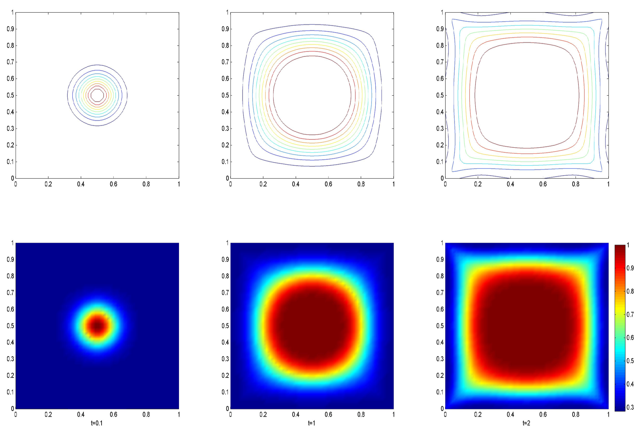
4.3. Five Spot Pattern Case

For the common whole five-spot pattern, $K=0.01$, we set the injection well in the center with an injection rate of $q=100$ and m${}^2$/s, and the production wells at the four corners with a production rate of $q=-25$ and m${}^2$/s.

The numerical velocity and pressure are shown in Figure 3, and the evolution of the invading fluid is presented in Figure 4.

4.4. Five-Spot Pattern with Random Permeability Case

Based on the five-spot pattern, we studied random permeability cases, where the range of bottom right-hand quarter was from $0.1$ to $0.5$ and others were from $1/7$ to $1/6$. Based on the results shown in Figure 5, we observed that the flow was faster along the domain with higher permeability. These examples showed that the multi-point flux MFE method was, indeed, effective for simulating a miscible displacement problem.

5. Results

We carried out four numerical experiments to verify the correctness of the theoretical analysis and the efficiency of the method. In Example 1, we tested the convergence order of the method, which was consistent with the theorem and corollary results. In the next three examples, we tested the application performance of the proposed method, based on water-oil miscible displacement problems involving a single injection and single production; a five-spot pattern; and random permeability five-spot pattern. The test results showed that the flow velocity along the high permeability area was relatively fast, which was reasonable.

6. Discussion

For compressible miscible displacement problems, a multi-point flux MFE decoupled method was considered. One of its advantages was that it avoided the coupled saddle-point problem by introducing a trapezoidal numerical integration formula. The BDM1 element was used for spatial discretization to approximate the velocity and the pressure, and a standard FE was used to approximate the concentration. A backward Euler scheme was proposed for the time discretization. The error estimates of the three variables were obtained through strict theoretical derivation, and the results were consistent with the convergence order in a previous incompressible article [15]. In the future, we will study another compressible miscible displacement problem, in which the velocity and pressure are controlled by the nonlinear Darcy–Forchheimer equation, since the non-Darcy and coupling problems actually exist in high-water cut reservoirs and areas with a high flow velocity around the well-bore.

References

1. Douglas, J., Jr.; Roberts, J.E. Numerical Methods for a Model for Compressible Miscible Displacement in Porous Media. Math. Comput. 1983, 41, 441–459. [Google Scholar] [CrossRef]
2. Feng, W.; Guo, H.; Kang, Y.; Yang, Y. Bound-preserving discontinuous Galerkin methods with second-order implicit pressure explicit concentration time marching for compressible miscible displacements in porous media. J. Comput. Phys. 2022, 463, 111240. [Google Scholar] [CrossRef]
3. Guo, H.; Yang, Y. Bound-Preserving Discontinuous Galerkin Method for Compressible Miscible Displacement in Porous Media. SIAM J. Sci. Comput. 2017, 39, A1969–A1990. [Google Scholar] [CrossRef]
4. Chuenjarern, N.; Xu, Z.; Yang, Y. High-order bound-preserving discontinuous Galerkin methods for compressible miscible displacements in porous media on triangular meshes. J. Comput. Phys. 2019, 378, 110–128. [Google Scholar] [CrossRef]
5. Li, A.; Huang, J.; Liu, W.; Wei, H.; Yi, N. A characteristic block-centered finite difference method for Darcy-Forchheimer compressible miscible displacement problem. J. Comput. Appl. Math. 2022, 413, 114303. [Google Scholar] [CrossRef]
6. Li, X.; Rui, H. Characteristic block-centered finite difference method for compressible miscible displacement in porous media. Appl. Math. Comput. 2017, 314, 391–407. [Google Scholar] [CrossRef]
7. Li, X.; Rui, H.; Xu, W. A new MCC-MFE method for compressible miscible displacement in porous media. J. Comput. Appl. Math. 2016, 302, 139–156. [Google Scholar] [CrossRef]
8. Zhang, J. A new combined characteristic mixed-finite-element method for compressible miscible displacement problem. Numer. Algorithms 2019, 81, 1157–1179. [Google Scholar] [CrossRef]
9. Hu, H. Two-grid method for compressible miscible displacement problem by mixed-finite-element methods and expanded mixed-finite-element method of characteristics. Numer. Algorithms 2022, 89, 611–636. [Google Scholar] [CrossRef]
10. Zeng, J.; Chen, Y.; Hu, H. Two-grid method for compressible miscible displacement problem by CFEM-MFEM. J. Comput. Appl. Math. 2018, 337, 175–189. [Google Scholar] [CrossRef]
11. Wheeler, M.F.; Yotov, I. A multi-point flux mixed-finite-element method. SIAM J. Numer. Anal. 2006, 44, 2082–2106. [Google Scholar] [CrossRef]
12. Wheeler, M.F.; Xue, G.; Yotov, I. Coupling multi-point flux mixed-finite-element methods with continuous galerkin methods for poroelasticity. Computat. Geosci. 2014, 18, 57–75. [Google Scholar] [CrossRef]
13. Arrarás, A.; Portero, L. Multipoint flux mixed-finite-element methods for slightly compressible flow in porous media. Comput. Math. Appl. 2019, 77, 1437–1452. [Google Scholar] [CrossRef]
14. Xu, W.; Liang, D.; Rui, H. A multi-point flux mixed-finite-element method for the compressible Darcy-Forchheimer models. Appl. Math. Comput. 2017, 315, 259–277. [Google Scholar] [CrossRef]
15. Xu, W.; Liang, D.; Rui, H.; Li, X. A Multipoint Flux Mixed Finite Element Method for Darcy-Forchheimer Incompressible Miscible Displacement Problem. J. Sci. Comput. 2020, 82, 1–20. [Google Scholar] [CrossRef]
16. Adams, R.A.; Fournier, J.J.F. Sobolev Spaces; Elsevier: Amsterdam, The Netherlands, 2003. [Google Scholar]
17. Ewing, R.E.; Russell, T.F.; Wheeler, M.F. Convergence analysis of an approximation of miscible displacement in porous media by mixed finite elements and a modified method of characteristics. Comput. Methods Appl. Mech. Eng. 1984, 47, 73–92. [Google Scholar] [CrossRef]
18. Brezzi, F.; Douglas, J., Jr.; Marini, L.D. Two families of mixed finite elements for second order elliptic problems. Numer. Math. 1985, 88, 217–235. [Google Scholar] [CrossRef]
Figure 1. The graphs of the concentration, pressure, and velocity fields of Example 4.1 .
Processes 11 01244 g001
Figure 2. Contours and graphs of concentration in single injection single production case.
Processes 11 01244 g002
Figure 3. The numerical velocity and pressure solution in five-spot pattern.
Processes 11 01244 g003
Figure 4. Contours and graphs of concentration in five-spot pattern.
Processes 11 01244 g004
Figure 5. Contours and graphs of concentration in random permeability case.
Processes 11 01244 g005