Article

Multi-Objective Multi-Stage Optimize Scheduling Algorithm for Nonlinear Virtual Work-Flow Based on Pareto

School of Computer Science and Technology, Harbin University of Science and Technology, Harbin 150080, China
*
Author to whom correspondence should be addressed.
Processes 2023, 11(4), 1147; https://doi.org/10.3390/pr11041147
Submission received: 6 March 2023 / Revised: 26 March 2023 / Accepted: 3 April 2023 / Published: 8 April 2023

Abstract

:
Work-flow scheduling is for finding the allocation method to achieve optimal resource utilization. In the scheduling process, constraints, such as time, cost and quality, need to be considered. How to balance these parameters is a NP-hard problem, and the nonlinear manufacturing process increases the difficulty of scheduling, so it is necessary to provide an effective heuristic algorithm. Aiming at these problems, a multi-objective nonlinear virtual work-flow model was set up, and a multi-objective staged scheduling optimization algorithm with the objectives of minimizing cost and time and maximizing quality was proposed. The algorithm includes three phases: the virtualization phase abstracts tasks and services into virtual nodes to generate a virtual work-flow model; the virtual scheduling phase divides optimized segments and obtains the solution set through reverse iteration; the generation phase obtains the scheduling path according to the Pareto dominance. The proposed algorithm performed 10.5% better in production quality than the minimum critical path algorithm, reduced the time to meet the time constraint by 9.1% and saves 13.7% more of the cost than the production accuracy maximization algorithm.

1. Introduction

Work-flow technology is a kind of automatic program flow that is used often for commercial and research purposes because of its efficient and clear organization of the work process. Exploiting work-flow technology, the manufacturing process can be interconnected, sharing data between production machines and analytics systems [1,2]. This increased flow of data enables a clear view in the manufacturing process, making it possible to automatically and better schedule processes.
With the development of technology and the change of consumer demand, enterprises are inclined toward personalized and non-standardized design and manufacturing [3]. In this kind of complex manufacturing system, the process route presents the characteristics of being nonlinear and highly selective. Current research focuses on solving scheduling problems from two aspects: problem models and solution methods [4,5,6]. Scheduling processes directly affect the efficiency and cost of manufacturing. Nonlinear manufacturing processes are constrained by the requirements of the production time, product quality and overhead costs. In addition, each customer may have different quality of service (QoS) requirements based on their workload. How to dynamically balance these parameters is an NP-hard problem [7].
Multi-objective optimization has become a hot research topic over the last decades, as it has been proven to be an easy and effective approach for solving real-world optimization problems [8]. The conflict within multi-objective optimization limits the scheduling direction of feasible solutions, and the existing algorithms have difficulty balancing the parameters or cannot find the optimal solution in solving the multi-objective nonlinear scheduling problem [9,10]. This paper proposes a heuristic approach to address this restriction in scheduling nonlinear manufacturing. We intend to determine a schedule for the tasks to select a proposal service. To obtain this schedule, we formulate a multi-objective optimization problem: the enterprises may seek a tradeoff among processing time, cost and quality. In this work, we establish the virtual work-flow model of the multi-objective nonlinear manufacturing process and propose a three-stage approach to solve the problem. The first stage is the virtualization stage; the core of this stage is simplification, and the nonlinear work-flow instance is abstracted to a non-linear virtual work-flow model. The second stage is the virtual scheduling stage; the work-flow is segmented, and each segment is scheduled through a backward reduction iteration to obtain the feasible solutions. The third stage is the generation stage; the solution set is obtained by forward scheduling, and the scheduling sequence is generated by the Pareto domination relation.

2. Related Work

According to the optimization objective, work-flow scheduling problems can be divided into single-objective optimization and multi-objective optimization. For single-objective optimization problems, scholars often use precise algorithms, heuristic algorithms and intelligent algorithms to solve problem. At present, most multi-objective optimization problems consider 2–3 optimization objectives. To solve these different problems, scholars usually use intelligent algorithms, heuristic algorithms, hybrid algorithms, etc. The problem of resource provisioning and scheduling has been extensively addressed in the literature by considering different perspectives. To achieve the optimal resource scheduling scheme, various scheduling algorithms have been proposed.
In paper [11], the authors proposed two scheduling heuristics for complex application jobs, which reduce scheduling overhead by reducing queue rearrangement and processing task priority constraints. In paper [12], the authors investigated the single-machine scheduling problem that considers the due date assignment and past-sequence-dependent setup times simultaneously, and they designed an algorithm that can jointly find the optimal sequence and optimal due dates. In paper [13], the authors proposed a Pareto-based, multi-objective, discrete Ant Lion Optimization Algorithm that involves a new encoding scheme for ants and antlions to address the discrete nature of work-flow scheduling. Subsequently, they used the Pareto dominance and crowding distance approach to tackle the optimization of multiple objectives and to achieve the optimal solutions. In paper [14], the authors used the multi-objective Black Widow Optimization Algorithm to solve the multi-objective optimization problem of a power system; the weighting factor method was adopted to handle the multi-objective optimal scheduling problem by simultaneously maximizing profit and minimizing emissions, while satisfying the related constraints. In paper [15], to deal with the combinatorial problem, the authors presented the three main phases of hybrid, discrete Particle Swarm Optimization, which combined with the Hill Climbing technique at the third phase to enhance the overall performance. In paper [16], the authors formulated the cyber–physical cloud systems work-flow scheduling problem under reliability, security and time constrains, and proposed a dependable hybrid scheduling scheme with statically scheduled tasks and dynamically assigned recoveries. In paper [17], the authors proposed a dynamic, deadline- and budget-aware work-flow scheduling algorithm that is designed for multiple instances or dynamic behavior work-flow in WaaS environments. In paper [18], a variable neighborhood search-based method and a hybrid heuristic method are developed to solve problems with practical order picking and a distribution system. In paper [19], the authors proposed an efficient priority and relative distance algorithm to minimize the task scheduling length for precedence-constrained work-flow applications without violating the end-to-end deadline constraint. In paper [20], based on a generalized backward strategy, the authors built timed Petri net models for two transient processes and derived two linear programs to search a feasible schedule with a minimal makespan. In paper [21], combining the merits of an artificial bee colony (ABC) and cuckoo search (CS) in a multi-cloud environment, the authors proposed a new resource provisioning model using the hybrid CS algorithm; the approach can provide seamless service to the users in an efficient manner. In paper [22], the authors propose an enhanced, multi-objective, harmony search algorithm and a Gaussian mutation to solve flexible flow shop scheduling problems with a sequence-based setup time, transportation time and probable rework. In paper [23], the authors proposed a Dynamic Multi-Stage Schedule Optimization Algorithm to seek a tradeoff among processing time, energy consumption and other cost functions in flexible manufacturing. In paper [24], after analyzing the combined effects of cloud uncertainty and probabilistic constraints, the authors proposed a customized Genetic Algorithm to minimize the expected work-flow execution time and monetary cost under probabilistic constraints on the deadline and budget. In paper [25], the authors proposed a multi-objective optimal dispatch model of an interconnected gas–electricity energy system, and an improved cuckoo algorithm is used to optimize the multi-objective scheduling model. In paper [26], the authors proposed a semi-multi-objective problem by considering intermediate storage with a tolerable maximum completion time, and a two-step evolutionary algorithm solution was proposed to solve the problem. In paper [27], the authors proposed an improved multi-objective Ant Lion Algorithm that aims to minimize the maximum completion time and energy consumption, and simultaneously optimize the maximum completion time, energy consumption cost and carbon emissions. In paper [28], based on the reliability assessment results, the authors designed a migration strategy, with reliability as the optimization goal while considering costs, and proposed a service function chain reliability evaluation method and reliability optimization algorithm. In paper [29], based on an improved version of the Rainfall Algorithm and the Salp Swarm Algorithm, the authors presented a novel scheduling scheme for real-time home energy management systems.

3. Problem Description

3.1. Work-Flow Definitions

Definition 1
(Original work-flow model W). Defined as W = <P,T,L,S>, where P is the process nodes set, denoted as P = (p0, p1,…,pn); T is the transfer node set, denoted as T = (t0, t1, …, tm); L is the directed edges set, denoted as L = (l0, l1, …, ly); S is the resources set, denoted as S = (s0, s1, …, sz), which corresponds to the optional resources of each transfer node, and each optional resource sk corresponds to the production attribute ai = (qi, ci, hi), including three parts, namely, production quality qi, production cost ci and production time hi.
Definition 2
(Virtual node p). Tasks in work-flow can be reconstructed to a virtual node, p′[i–j] denotes the virtual node is reconstructed from node pi to pj, and p′[i,j] denotes the virtual node is reconstructed of the adjacent node pi and pj. In addition, the virtual nodes pb and pe are set in the virtual work-flow model to represent the beginning and end of the business process.
Definition 3
(Virtual work-flow VW). Defined as VW(W, DP, P′, T′, Id, Od), where VW is obtained from the original work-flow model W through virtualization; DP is the abstract set of detection nodes set in the model according to the process requirements, denoted as DP = (dp1, dp2 … dpi … dpk); dpi = (σiq, σic) indicates that when the work-flow is executed to detection department i, the quality pass rate σiq and cost pass rate σic are set in this node according to the process requirements, and the cumulative production quality fw(pj, hj) and cumulative production cost fc(pj, hj) of the precursor process node pj are detected respectively. If the σiq is met, the work-flow will continue to execute; otherwise, it will enter the feedback path for adjustment until the σiq is met. Id is the abstract set of in-degree of each node, denoted as Id = (id1, id2 … idi … idz); Od is the abstract set of the out-degree of each node, denoted as Od = (od1, od2 … odi … odz). P′ is the abstract process nodes set through reconstruction, denoted as P′ = (p1′, p2′ … pi′ … pn′); T′ is the virtual transfer node set after reconstruction, denoted as T′ = (t1′, t2′ … ti′ … tm′).
Definition 4
(Virtual work-flow diagram VG). Defined as VG(VW, E), where E is the abstract set of directed edges reflecting the dependencies of the nodes in VW, denoted as E = (e1, e2 … ei … en).
Definition 5
(Manufacturing expectation ME). Refers to the product parameters that the manufacturing process represented by the nonlinear work-flow expects to obtain when the product is delivered. Set ME = (H, C, Q), where H is the time constraint, the latest completion time of the work-flow; C is the cost constraint, the cost limit of the selected processing service; Q is the production quality constraint, the minimum quality to be achieved when the product is delivered.
Definition 6
(Task interval TFi). TFi reflects the time range in which process node pi can choose the optimal manufacturing service, and is denoted as TFi[FBi,FEi], which can be calculated by Equation (1), where FBi is the earliest start time of process node pi, FEi is the latest start time of process node pi, FBq is the direct predecessor of process node pi, and FEp is the direct successor.
F B i = Max F B i 1 + Min h i j , F B i 1 , F B q , k F E i = Min F E i 1   Min h i j , F E i 1 , F E p , l F B 1 = 0 , F E n = M E . H s . t . k = 1 , 2 , , i d i ; l = 1 , 2 , , o d i
Definition 7
(The execution domain θ). θ = [θminmax] is the manufacturing interval of the virtual node transformed by the partial virtual node P’(P’ ∈ P) in the reconstructed virtual work-flow graph VG, which can be obtained from Equation (2).
θ min = max { F B j F B i } θ max = min { F E j F B i }
Definition 8
(Special different path SDP). If there exists a node pi in the virtual work-flow graph VG with Od > 1, which can be reconstructed with node pj as a virtual node p’[i,j], but another out-degree of node pi can be reconstructed with node pk as another virtual node p’[i,k], then the path formed by pi and pk is SDP.
Definition 9
(Manufacturing attribute A). Defined as A = (AQp, ACp, AHp), it represents the cumulative production attributes at node p, including the cumulative production quality AQp, cumulative production cost ACp and cumulative production time AHp. It can be calculated by Equation (3), where q is the predecessor node of node p, when lij = 1 denotes the selection of the corresponding resource in the manufacturing resource set, and when p = E denotes that the scheduling is complete; AE denotes the final manufacturing attribute.
A H p = Max , A H p , k + l p j h q j M E . H A C p = Max , A C p , k + l p j c p j M E . C A Q p = n i N l i j w i j M E . Q s . t . j = 1 k l i j = 1 , l i j 0 , 1 , q < p , k = 1 , 2 , , i d p

3.2. Nonlinear Virtual Work-Flow Model VWF Generation Algorithm

The essence of the work-flow scheduling problem is to establish the mapping relationship between multiple tasks and optional services. In order to improve the resource waste and time loss caused by irrational process selection in the nonlinear manufacturing process, this paper proposes a virtual stage scheduling model of nonlinear work-flow, which is composed of three parts: virtual work-flow model, virtual work-flow diagram and manufacturing resource set, which can be defined as VWF(Re, Map, VW, VG), where Re is the manufacturing resources set consisting of the set P and the set T; Map is the set of mapping relations from the set of manufacturing resources to the model VW, which can be expressed as Map = (map1, map2 … mapi …, mapn + m).
When users submit work-flow tasks and requirements, the available resources in each task and resource collection are abstracted to form a virtual manufacturing resource collection, which is mapped to the virtual work-flow after virtualization. Tasks with associated dependencies are divided according to the manufacturing process characteristics and actual requirements, and detection nodes are preset to schedule tasks in each phase one by one to generate a virtual work-flow graph. Combined with previous research [7], the design modeling algorithm of the nonlinear virtual work-flow model VWF is as follows.
Step 1
Abstract the production as the process node set P and T, the optional resources corresponding to the conversion form as resource set S, and the partial order relationship of each process node as directed edge set L to construct the original work-flow model W.
Step 2
Add the set of detection nodes DP and the virtual nodes PB and PE to the work-flow model W and update the set of directed edges L.
Step 3
Input process nodes with od or id greater than 1 into the Queue, except for the feedback predecessor structure.
Step 4
Output the process node pj with od > 1 in Queue, find the nearest feedback in-degree process node pi, and delete all process nodes between pi and pj from the queue.
Step 5
Reconstruct all process nodes between nodes pi and pj, save node pi temporarily to the virtual process node set P′, reconstruct the transfer nodes involved in this process as virtual transfer nodes, and save them to the virtual transfer node set T′.
Step 6
Iterate virtual process node pi in the set P′ and determine whether there is an SDP generated due to virtual reconstruction. If so, divide the virtual process node pi and the virtual transfer node ti and restore the process nodes and transfer nodes that constitute the virtual node. Otherwise, delete the pi and ti, repeat until the set P′ or T′ is empty, and then output the VW.
Step 7
Traverse model VW; count all paths from adjacent process node pi to pj(pipj); establish directed edge ejk, where k = 1, 2,…, idpj; calculate the parameters hjk, cjk and qjk of directed edge ejk; and mark these parameters to form a virtual work-flow diagram VG.

3.3. Virtual Work-Flow Example

The production process of a sheet metal workshop contains process classification, part programming, machine setup, cutting, mass production, quality inspection and other links. It can be extracted as a set of 12 process nodes P and the corresponding set of transfer nodes T, as shown in Table 1.
The production process presents nonlinear characteristics. A nonlinear virtual work-flow can be used to optimally schedule its production time, production quality and production cost, with multiple objectives, and input the information of each node into the model generation algorithm VWF to obtain the work-flow model shown in Figure 1.
According to the requirements of users, the principal tasks and the corresponding services are extracted from the production process as a process node set P and a transfer node set T, and their execution order is mapped to the original work-flow graph. On this basis, according to the virtualization rules, the nodes are transformed into virtual nodes, and the directed edge relationship is reconstructed to generate a virtual work-flow graph to decide the execution order of each task.

4. Multi-Objective Nonlinear Virtual Work-Flow Staged Scheduling Algorithm Based on Pareto Optimization

Definition 10
(Pareto optimal). Refers to an ideal state of manufacturing resource allocation, which is the equilibrium point of the optimal strategy. In the process of moving from one allocation state to another, making one attribute improve without making another attribute decrease is called Pareto improvement, and the state where there is no Pareto improvement is called Pareto optimal.
Definition 11
(Pareto domination). Suppose there are functions ƒq with the objective of maximizing the cumulative production quality AQp and functions ƒc and ƒh with the objectives of minimizing the cumulative production time AHp and cumulative production cost ACp. xi = (p1/t1Sk, p2/t2Sk, …, pn/tnSk) and xj = (p1/t1Sk, p2/t2Sk, …, pn/tnSk) are two sets of solution vectors consisting of the process node pi and the transfer node tiSk on this path. When fq (xi) ≥ fq (xj), fh (xi) ≤ fh (xj), fc (xi) ≤ fc (xj) and at least one of the strict inequalities holds, the solution vector xi dominates the solution vector xj, denoted as xi > xj.
Definition 12
(Pareto-optimal solution). Let X be the set of feasible solutions of a multi-objective optimization problem, and the set of solutions of all Pareto feasible solutions constitutes the Pareto optimal solution set of this multi-objective optimization problem. xi is a Pareto optimal solution if there is no xj in X, such that all the objective attributes corresponding to xi are elevated.
Assuming that the functions ƒq(pi,hpi) and ƒc(pi,hpi) denote the highest production quality and lowest cost, respectively, of process node pi(piP′) selected in its task interval TFi[FBi,FEi] at moment hpi for the virtual work-flow, ƒq(pi,hpi) and ƒc(pi,hpi) can be calculated using Equation (4).
ƒ q ( p i , h p i ) = max { q p i k } ƒ c ( p i , h p i ) = min { c p i k } h p i T F p i F B p i , F E p i , 0 < k i d p i s . t . h p i + h p i k M E . H , c p i + c p i k M E . C , w p i × w p i k M E . Q
Let pj be the precursor node of process node pi(piP′,pjP′) and use Equation (5) to calculate the cumulative production quality and cost of node pj.
ƒ q ( p j , h p j ) = max { f q ( p i , h p j + h p i ) × q p j k } ƒ c ( p i , h p j ) = min { f c ( p i , h p j + h p i ) + c p j k } h p j T F p j F B p j , F E p j , 0 < k i d p j s . t . h p j + h p j k M E . H , c p j + c p j k M E . C , w p j × w p j k < M E . Q
The calculation of each attribute of the last task of each layer can be completed using Equation (4), and then combined with Equation (5), can be iterated backwards to calculate the cumulative attributes obtained by scheduling resources for each task within the maximum range allowed by the task interval TFi.
The Multi-objective Nonlinear Virtual Work-flow Staged Scheduling Algorithm (VWFA) uses virtual technology to transform tasks into virtual nodes, which are used as the basis for the subsequent simplification and merging of serial and feedback paths. The relative execution order of tasks in different stages in the optimization segment is limited by the task interval to ensure that the constraints are met and the available resources are scheduled in the maximum range. The results of the backward iteration are integrated to form a feasible solution set, and the feasible solutions are ranked according to the Pareto dominance relation, which can avoid the local optimal solution or the unreasonable local resource allocation caused by the limitation of local parameters, and select the optimal scheduling scheme that meets the needs of users. Based on the above strategy, the steps of algorithm VWFA are as follows.
Step 1
Invoke the modeling algorithm VWF to process each parameter of the nonlinear manufacturing process and form a nonlinear virtual work-flow model.
Step 2
Combine the manufacturing expectations ME and manufacturing characteristics to reverse the work-flow hierarchy, mark the last node of each layer, traverse backwards to the virtual node PB, and analyze and calculate the task interval TFi of each process node pi formed by each layer using Equation (1).
Step 3
Compute and mark the ƒw(E0,hE0) and ƒc(E0,hE0) of the process node E0 of the ending layer at each moment within its active interval TFi using Equation (4).
Step 4
Traverse the process nodes set P and determine whether there is an SDP. If not, then process the nodes at each stage, combine the process nodes on the serial path as virtual nodes pi, use Equation (4) to calculate the ƒq(pi,hpi) and ƒc(pi,hpi) available to the virtual node at each moment in its execution domain, and record the local feasible solution path. If it exists, however, turn to Step 5.
Step 5
If SDP exists, first calculate the execution domain θ of SDP using Equation (2), then calculate ƒq(pi,hpi) and ƒc(pi,hpi) available at different moments for each process node in this domain using Equation (4), and record the local feasible solution path.
Step 6
If the cumulative production parameters fail to meet the requirements when executed to detect node dp, a feedback correction is made, and the scheduling results are adjusted according to the dp, and some scheduling strategies are eliminated.
Step 7
Using Equation (3) with manufacturing expectation ME as a constraint, fully process the set of marked model process nodes P and deposit the feasible scheduling sequence into the Pareto solution set X according to the stage accumulation rule.
Step 8
Determine the dominance relationship based on the manufacturing attributes of each scheduling sequence in the Pareto solution set X and output the optimal scheduling route x*.

5. Algorithm Analysis

5.1. Experimental Environment and Data

The server operating system used for the experiments was Windows Server 2016, with a memory configuration of 4G. The VWF model and the optimized scheduling algorithm VWFA code were constructed in Java. To verify the performance of the optimization algorithm, a sheet metal shop production example described in Section 3.3 was chosen for analysis, setting the manufacturing expectation as ME = (Q, C, H) = (0.93, 50, 51) and a batch of sheet metal production parameters, as shown in Table 2.
After inputting the process model shown in Figure 1 and the data shown in Table 2 into the algorithm VWFA, the optimal solution x* that conforms to the Pareto dominance rule is formed by the process shown in Figure 2.

5.2. Model Optimization Process

The scheduling process in Figure 1 is divided into three optimization segments based on the characteristics of this sheet metal manufacturing process. ME.H = 51 day, and the time constraints of the three optimized sections are set as follows: the first section is equipment commissioning ME.H1 = 6, the second segment is primary process machining ME.H2 = 25, and the third segment is finish machining ME.H3 = 20. According to the requirements set in the detection set DP = {dp1, dp2, dp3}, in the first segment to detect the equipment commissioning situation, set the detection point dp1 = (σ1q, σ1c), where σ1q = 0.980, σ1c = 2.5; when converting to this detection node, if ƒq(pi,hpi) < 0.980, it is necessary to feedback to the precursor node to recommission the equipment with a delay of 1 day, increasing the cost by 0.5 thousand dollars and eliminating the current scheduling scheme if ƒc(pi,hpi) ≥ 3 thousand dollars. In the second segment, to detect the primary process machining, set the detection node dp2, where σ2q =0.950; when converting to this detection node, if ƒq(pi,hpi) < 0.950, it needs to be fed back to the precursor node to adjust the processing, delaying 2 days and costing an additional 5 thousand dollars with no cost constraint. Set the detection node dp3 in the third segment, where σ3q =0.970; when converting to this node, if ƒq(pi,hpi) < 0.970, feedback to the predecessor node to adjust the processing, which delays 2 days and costs an additional 3 thousand dollars with no cost constraint. The selected scheduling scheme should satisfy ƒc(pi,hpi) ≤ 50 thousand dollars. The manufacturing attributes of each segment can be passed cumulatively, and the calculation procedure to obtain the Pareto solution set X according to the VWFA algorithm is as follows.
In the first optimization segment, according to Equation (1), the active intervals of process nodes p1, p2 and p3 are respectively TF1 = [0,2], TF2 = [2,4] and TF3 = [3,5]. The ƒq and ƒc of process nodes p1, p2 and p3 that start at the different moments hpi are as follows.
Calculation process of process node p3:
  • ƒq(p3,5) = max{0.97} = 0.970; ƒc(p3,5) = 0.3;
  • ƒq(p3,4) = max{0.97} = 0.970; ƒc(p3,4) = 0.5;
  • ƒq(p3,3) = max{0.97,0.99} = 0.990; ƒc(p3,3) = 0.5.
Calculation process of process node p2:
  • ƒq(p2,4) = max{0.98 × ƒq(p3,5)} = 0.951; ƒc(p2,4) = 1.2;
  • ƒq(p2,3) = max{0.98 × ƒq(p3,4)} = 0.970; ƒc(p2,26) = 1.2;
  • ƒq(p2,2) = max{0.98 × ƒq(p3,3)} = 0.970; ƒc(p2,25) = 1.2.
Calculation process of process node p1:
  • ƒq(p1,2) = max{0.94 × ƒq(p2,4)} = 0.894; ƒc(p1,2) = 0.2;
  • ƒq(p1,1) = max{0.94 × ƒq(p2,3),0.96׃q (p2,4)} = 0.913; ƒc(p1,1) = 0.3;
  • ƒq(p1,0) = max{0.94 × ƒq(p2,2),0.96׃q (p2,3)} = 0.931; ƒc(p1,0) = 0.3.
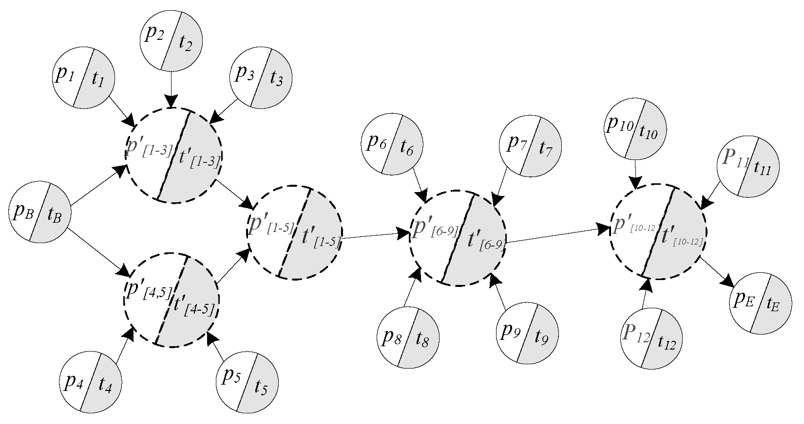
The above process shows that the reverse iteration to p1 in this domain produces three local scheduling paths with a cumulative production quality of ƒq(p1,0) = 0.931, ƒq(p1,1) = 0.913 and ƒq(p1,2) = 0.894; the cumulative production times are 6, 5 and 5, and the cumulative production costs are 2, 1.8 and 1.7, respectively. According to the rules described in Definition 8, it is reconstructed as a virtual process node p′[1–3], and the execution domain of p′[1–3] is obtained according to Equation (2): θ1 = [3,5]. The scheduling process and results of p′[1–3] is in Table 3.
Record the feasible solutions path1a1 and path1a2 for the first optimization segment according to Table 3. The serial path consisting of p4 and p5 in the first optimization segment without detection nodes produces two locally feasible solutions: path1b1 and path1b2, reverse scheduling to p4 with cumulative production quality and cost of ƒq(p4,0) = 0.940 and ƒc(p4,0) = 1.9, ƒq(p4,0) = 0.960 and ƒc(p4,0) = 2.1, respectively. Cross-combining the locally feasible solutions, four locally feasible solutions, namely, path11, path12, path13 and path14, are obtained.
The second optimization segment according to Equation (1) yields the active intervals of process nodes p6, p7, p8 and p9 as TF6 = [0,5], TF7 = [1,6], TF8 = [3,8] and TF9 = [18,23], respectively. The ƒq of process nodes p6, p7, p8 and p9 at the different start moments hpi are calculated with the same strategy in the first segment. Six local scheduling paths are generated when the reverse iteration is to p6. With the cumulative production quality of ƒq(p6,0) = 0.857, ƒq(p6,1) = 0.857, ƒq(p6,2) = 0.830, ƒq(p6,3) = 0.822, ƒq(p6,4) = 0.796 and ƒq(p6,5) = 0.779, the cumulative production times used are 24, 24, 23, 22, 21 and 20, respectively. According to the rules described in Definition 8, the path meets the virtual reconstruction requirements, and there is no SDP, so it is reconstructed as a virtual process node p′[6–9], and the execution domain of p′[6–9] is obtained according to Equation (2): θ2 = [18,23]. The scheduling process and results of p′[6–9] are shown in Table 4.
The corrected cumulative production quality is ƒq(p6,2) = 0.971, ƒq(p6,3) = 0.968, ƒq(p6,4) = 0.958 and ƒq(p6,5) = 0.951, and 4 locally feasible solutions, namely, path21, path22, path23, and path24, are recorded.
The third optimization segment according to Equation (1) yields the active intervals of process nodes p10, p11 and p12 as TF10 = [0,4], TF11 = [3,7] and TF12 = [13,17], respectively. The ƒq and ƒc of process nodes p10, p11 and p12 at different start moments hpi are calculated with the same strategy in the first segment, and 5 local scheduling paths are generated, with ƒq(p10,0) = 0.903, ƒq(p10,1) = 0.883, ƒq(p10,2) = 0.875, ƒq(p10,3) = 0.860 and ƒq(p10,4) = 0.823, and the cumulative production times are 21, 20, 19, 18 and 17, respectively. According to the rules described in Definition 8, the path meets the virtual reconstruction requirements, and it is reconstructed as a virtual process node p′[10–12], and the execution domain of p′[10–12] is obtained according to Equation (2): θ3 = [13,17]. The scheduling process and results of p′[10–12] are shown in Table 5.
The paths whose cumulative production quality does not meet the requirements of σ3q are fed back to the corresponding nodes for correction. The paths starting from moments 0 and 1 are eliminated due to the corrected cumulative production time exceeding ME.H3, and the corrected cumulative production quality is ƒq(p10,2) = 0.984, ƒq(p10,3) = 0.980 and ƒq(p10,4) = 0.969; the cumulative production cost is 18.5, 18.5, 18.6 and 18.6, which meets the requirement of σ3c; and the three local feasible solutions path31, path32 and path33 are recorded.

6. Algorithm Process and Results Analysis

6.1. VWFA Reconstruction Process

The VWFA algorithm divides the set of process nodes P in the VWF model into three optimization segments according to the process characteristics, none of the three optimized segments has SDP, and the process nodes of the three optimized segments are fictitiously formed into p′[1–5], p′[6–9] and p′[10–12] according to the rules. The virtual reconstruction process of the VWFA algorithm is shown in Figure 3.
Table 6 shows the local feasible solutions generated by the three optimization segments. On the basis of the characteristics of the accumulative transferability of the manufacturing attributes in each segment, the scheduling solutions of the three optimization segments are cross-integrated to obtain a Pareto solution set X.
Take the ƒq, ƒc and ƒh as the object function. According to the domination rule in Definition 11: determine the dominant relation of each feasible solution; the solution without Pareto improvement is the optimal solution; the Pareto optimal solution x* = path11path21path31 is obtained; the final cumulative ƒq = 0.947, ƒc = 50.5 and ƒh = 50. Under this resource allocation and scheduling strategy, one can get the optimal equilibrium property.

6.2. Results Analyses

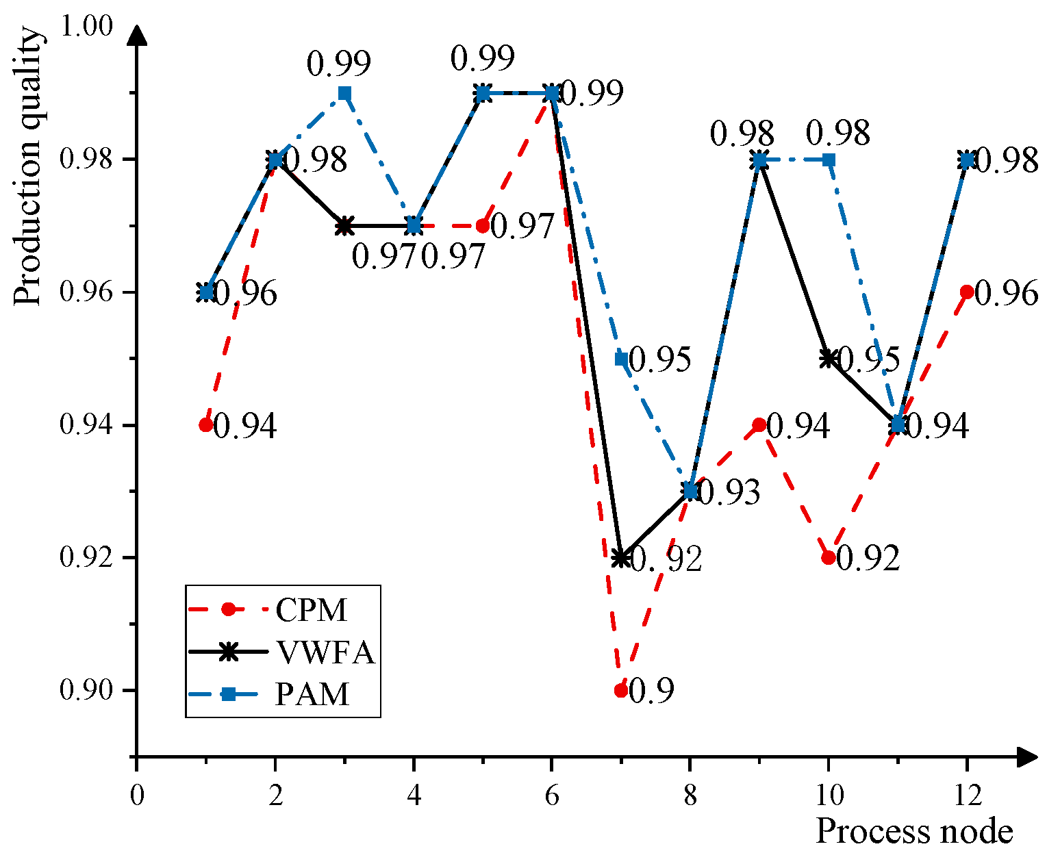
The data from the example described in Section 3.3 and Table 2 are input into the minimum critical path algorithm (CPM) and the production accuracy maximization algorithm (PAM). To ensure the validity and fairness of the comparison results, all three algorithms use the experimental environment described in Section 5.1 and set the placement manufacturing expectation ME = (Q, C, H) = (0.93,50,51). Three different scheduling paths path were obtained, as shown in Figure 4.
According to the scheduling path shown in Figure 4, the CPM or PAM algorithm has the deficiency of the single optimization goal or the lack of prediction in service selection. The VWFA algorithm determines the executable range of each task by dividing the work-flow into scheduling segments and calculating the execution domain of the virtual tasks. In this domain, the service selection scheme of each task under different conditions is simulated to expand the solution space and avoid the imbalance of overall resource allocation caused by the optimization of the local tasks. Finally, the optimal solution of time, cost and quality balance is obtained. Table 7 compares the scheduling results of the three algorithms.
Compared with CPM, the optimized production quality improvement of VWFA under the constraint of expectations is Δ = (ƒq − ƒq1)/ƒq1 × 100% = 10.5%. Compared with PAM, VWFA reduces the time by 9.1% to meet the time constraint and saves 13.7% of the cost. This result demonstrates that the algorithm VWFA has scheduling advantages under a limited range of EC constraints.

7. Impact of Other Parameters on the Performance of VWFA

7.1. Impact of the Number of Process Nodes

Since the algorithm is influenced by many factors during execution, this paper only investigates two important influencing factors: the number of process nodes and the performance impact of the finite range of engineering expectations EC.H on the algorithm.
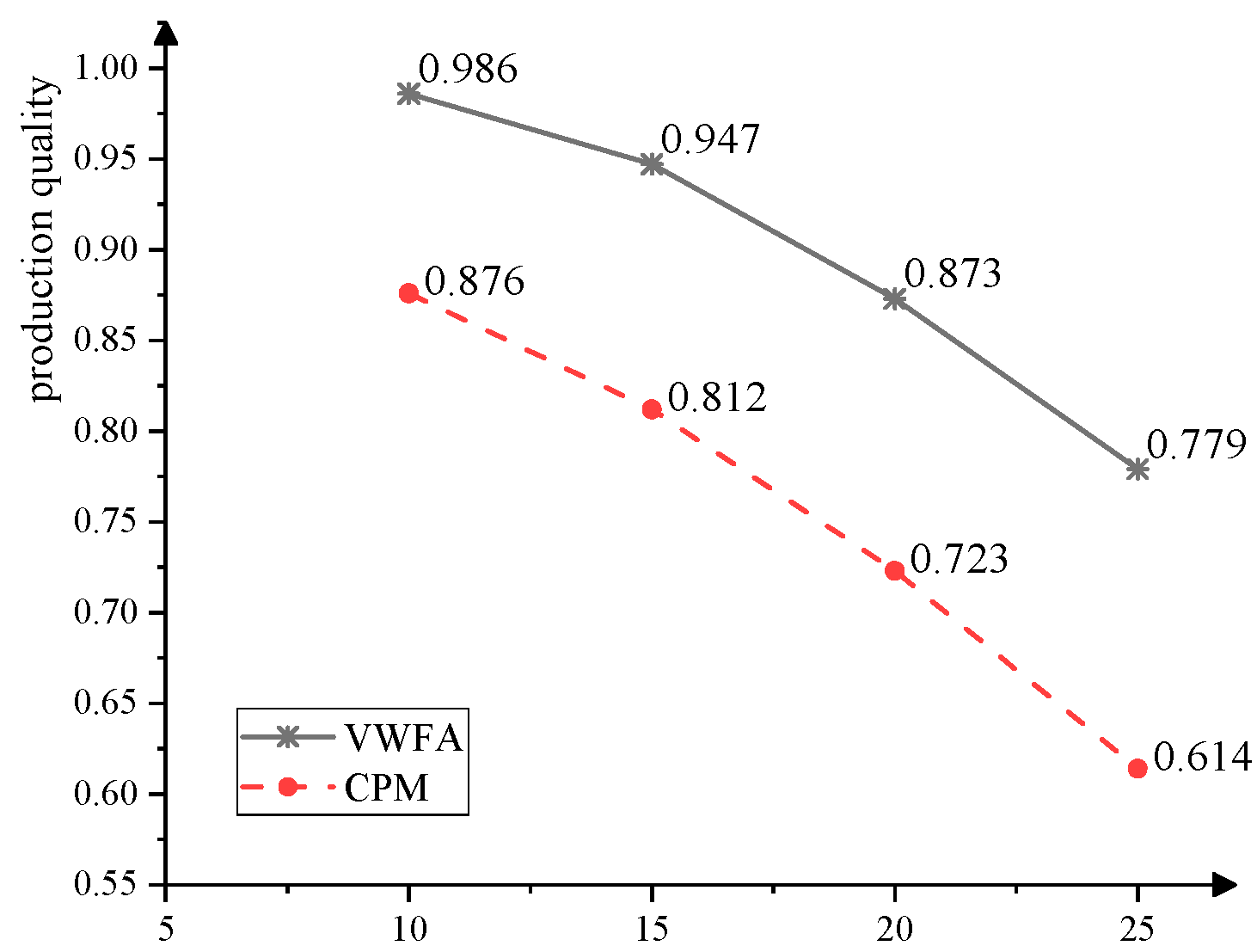
The cumulative production quality of the work-flow model is directly influenced by the production quality of each process node. A random number containing {10, 15, 20, 25} process nodes set P, corresponding to the number of {1, 2, 3, 4, 5} in the transfer node set T, is randomly generated. The effect of the change in the number of process nodes on the performance of the CPM and VWFA algorithms is shown in Figure 5.
Figure 5 shows that the number of process nodes is inversely proportional to the cumulative production quality ƒq. Compared with the CPM algorithm, the algorithm VWFA proposed in this paper improves on the cumulative production quality ƒq by 12.6%, 17.1%, 20.7% and 26.8%, respectively.

7.2. Impact of Time Constraints on Algorithm Performance

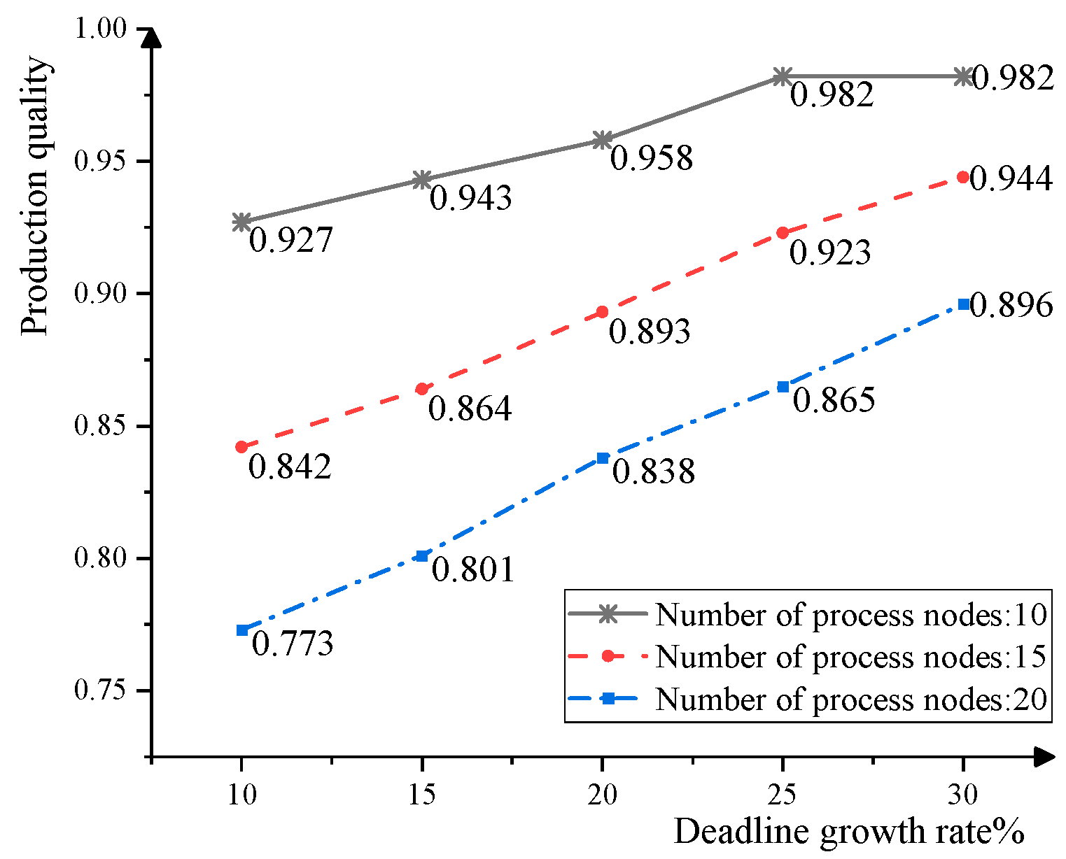
The deadline is the latest completion time of the business process, and usually the production quality increases with the increase of the time constraint. Randomly generating {10,15,20} process nodes, the number of service pools Si is taken from the interval [2,5] for any integer, increasing the deadline EC.H proportionally to 10%, 15%, 20%, 25% and 30% as the deadline and analyzing the impact on the algorithm VWFA. The results are shown in Figure 6.
In Figure 6, the experimental results show an increase in production quality as the deadline is delayed. The reason is that with the increase of the deadline, so does the execution domain increase, which means that some tasks can choose services with production accuracy. Therefore, the deadline can be increased appropriately to improve the efficiency of the algorithm.

8. Conclusions

Because of the complexity of a multi-objective nonlinear process, it is difficult to obtain high-quality solution results by a single-objective algorithm. This paper proposes a virtual work-flow model, VWF, and a staged scheduling optimization algorithm, VWFA, to address this challenge. The complex paths in the nonlinear work-flow are simplified and combined by virtualization, and the work-flow is divided into multiple optimization segments. To ensure the constraints can be satisfied and the utilization of resources can be maximized, the execution domain of the task is calculated to expand the solution space and avoid insufficient local resource scheduling. The feasible solution is obtained by combining backward and forward scheduling, and the optimal solutions satisfying the multi-objective optimization are selected according to the Pareto domination relation. The experimental results analysis shows that our approach performed better than the CPM and PAM algorithms. Using the proposed algorithm can provide a scheduling scheme to the users in an efficient manner, but there is still room for improvement. For example, when task parameters change due to proficiency or workpiece wastage, the effect of parameter changes on the algorithm should also be considered. In the future, we plan to include an adjustment strategy to improve the robustness of the algorithm and to provide better QoS.

Author Contributions

Conceptualization, Z.L. and X.L.; methodology, Z.L.; software, S.T.; validation, Z.L., X.L. and S.T.; formal analysis, X.L.; investigation, H.X.; resources, H.X.; data curation, J.L.; writing—original draft preparation, X.L.; writing—review and editing, X.L.; visualization, X.L.; supervision, Z.L.; project administration, J.L.; funding acquisition, Z.L. All authors have read and agreed to the published version of the manuscript.

Funding

This research was funded by the Heilongjiang Provincial Natural Science Foundation of China (No. LH2021F030).

Data Availability Statement

The data that support the findings of this study are available within the article.

Conflicts of Interest

The authors declare no conflict of interest.

References

  1. Wang, L.; Ren, Y.; Qiu, Q.; Qiu, F. Surveyon Performance Indicators for Multi-Objective Evolutionary Algorithms. Chin. J. Comput. 2021, 44, 1590–1619. [Google Scholar]
  2. Chao, L.; Fajun, Y.; Lu, Z. Efficient scheduling approaches to time-constrained single-armed cluster tools with condition-based chamber cleaning operations. Int. J. Prod. Res. 2022, 60, 3555–3568. [Google Scholar]
  3. Lu, R.; Zhu, C.; Cai, H.; Zhou, J.; Jiang, J. Time optimization for work-flow scheduling based on the combination of task attributes. J. Southeast Univ. 2020, 36, 399–406. [Google Scholar]
  4. Yuan, F.; Huang, B.; Wang, J. A Survey of Modeling and Scheduling of Cluster Tools Based on Petri Nets. Acta Autom. Sin. 2022, 45, 1–20. [Google Scholar]
  5. Menaka, M.; Kumar, K.S.S. Workflow scheduling in cloud environment–Challenges, tools, limitations & methodologies: A review. Meas. Sens. 2022, 24, 100436. [Google Scholar]
  6. Song, C. Improved NSGA-II algorithm for hybrid flow shop scheduling problem with multi-objective. Comput. Integr. Manuf. Syst. 2022, 28, 1777–1789. [Google Scholar]
  7. Luo, Z.Y.; Zhu, Z.H.; You, B.; Liu, J.H. Virtual iterative reduction optimization algorithm of work-flow’s time-accuracy. J. Electron. Inf. Technol. 2018, 40, 2013–2019. [Google Scholar]
  8. Zhou, W.; Xie, Z. Resource Collaborative Integrated Scheduling Algorithm Considering Multi-process Equipment Weight. J. Electron. Inf. Technol. 2022, 44, 1625–1635. [Google Scholar]
  9. Liu, C.; Li, J.; Liu, J.; Jiao, L. A Survey on Dynamic Multi-Objective Optimization. Chin. J. Comput. 2020, 43, 1246–1278. [Google Scholar]
  10. Qiao, Y.; Zhang, S.; Wu, N. Efficient Approach to Failure Response of Process Module in Dual-Arm Cluster Tools with Wafer Residency Time Constraints. IEEE Trans. Syst. Man Cybern. 2021, 51, 1612–1629. [Google Scholar] [CrossRef]
  11. Stavrinides, G.L.; Karatza, H.D. Multicriteria scheduling of linear work-flows with dynamically varying structure on distributed platforms. Simul. Model. Pract. Theory 2021, 112, 369–377. [Google Scholar] [CrossRef]
  12. Wang, X.; Liu, W.; Li, L.; Zhao, P.; Zhang, R. Due date assignment scheduling with positional-dependent weights and proportional setup times. Math. Biosci. Eng. 2022, 19, 5104–5119. [Google Scholar] [CrossRef]
  13. Rama, R.; Ritu, G. Pareto based ant lion optimizer for energy efficient scheduling in cloud environment. Appl. Soft Comput. 2021, 113, 943–962. [Google Scholar]
  14. Pandey, A.K.; Jadoun, V.K.; Sabhahit, J.N. Real-Time Peak Valley Pricing Based Multi-Objective Optimal Scheduling of a Virtual Power Plant Considering Renewable Resources. Energies 2022, 16, 5970. [Google Scholar] [CrossRef]
  15. Shirvani, M.H. A hybrid meta-heuristic algorithm for scientific work-flow scheduling in heterogeneous distributed computing systems. Eng. Appl. Artif. Intell. 2020, 90, 501–532. [Google Scholar]
  16. Zhou, J.; Sun, J.; Zhang, M.; Ma, Y. Dependable Scheduling for Real-Time Work-flows on Cyber–Physical Cloud Systems. IEEE Trans. Ind. Inform. 2021, 17, 7820–7829. [Google Scholar] [CrossRef]
  17. Saeedizade, E.; Ashtiani, M. DDBWS: A dynamic deadline and budget-aware work-flow scheduling algorithm in work-flow-as-a-service environments. Supercomput 2021, 77, 14525–14564. [Google Scholar] [CrossRef]
  18. Wang, S.; Wu, R.; Chu, F.; Yu, J. Variable neighborhood search-based methods for integrated hybrid flow shop scheduling with distribution. Soft Comput. 2019, 24, 8917–8936. [Google Scholar] [CrossRef]
  19. Zhang, L.; Zhou, L.; Salah, A. Efficient scientific work-flow scheduling for deadline-constrained parallel tasks in cloud computing environments. Inf. Sci. 2020, 531, 31–46. [Google Scholar] [CrossRef]
  20. Yang, F.; Qiao, Y.; Gao, K.; Wu, N.; Zhu, Y.; Simon, I.W.; Su, R. Efficient Approach to Scheduling of Transient Processes for Time-Constrained Single-Arm Cluster Tools with Parallel Chambers. IEEE Trans. Syst. Man Syst. 2020, 50, 3646–3657. [Google Scholar] [CrossRef]
  21. Kumar, K.S.S.; Jaisankar, N. Towards data centre resource scheduling via hybrid cuckoo search algorithm in multi-cloud environment. Int. J. Intell. Enterp. 2017, 4, 21–35. [Google Scholar] [CrossRef]
  22. Gheisariha, E.; Tavana, M.; Jolai, F.; Rabiee, M. A simulation optimization model for solving flexible flow shop scheduling problems with rework and transportation. Math. Comput. Simul. 2021, 180, 152–177. [Google Scholar] [CrossRef]
  23. Balszun, M.; Hobbs, C.; Fraccaroli, E.; Roy, D.; Chakraborty, S. Exploiting Process Dynamics in Multi-Stage Schedule Optimization for Flexible Manufacturing. In Proceedings of the 2022 IEEE 27th International Conference on Emerging Technologies and Factory Automation (ETFA), Stuttgart, Germany, 6–9 September 2022; IEEE: Piscataway, NJ, USA, 2022; pp. 1–8. [Google Scholar]
  24. Calzarossa, M.C.; Della Vedova, M.L.; Massari, L.; Nebbione, G.; Tessera, D. Multi-objective optimization of deadline and budget-aware workflow scheduling in uncertain clouds. IEEE Access 2021, 9, 89891–89905. [Google Scholar] [CrossRef]
  25. Yang, B. Multi-objective optimization of integrated gas–electricity energy system based on improved multi-object cuckoo algorithm. Energy Sci. Eng. 2021, 9, 1839–1857. [Google Scholar] [CrossRef]
  26. Kusuma, P.D.; Albana, A.S. A Parallel Permutation Flow-Shop Scheduling Model by Using a Two-Step Evolutionary Algorithm to Minimize Intermediate Storage with Tolerable Maximum Completion Time. Int. J. Intell. Eng. Syst. 2021, 14, 464–475. [Google Scholar]
  27. Geng, K.; Ye, C.; Dai, Z.H.; Liu, L. Bi-objective re-entrant hybrid flow shop scheduling considering energy consumption cost under time-of-use electricity tariffs. Complexity 2020, 2020, 8565921. [Google Scholar] [CrossRef] [Green Version]
  28. Rui, L.; Chen, X.; Gao, Z.; Li, W.; Qiu, X.; Meng, L. Petri Net-Based Reliability Assessment and Migration Optimization Strategy of SFC. IEEE Trans. Netw. Serv. Manag. 2021, 18, 167–181. [Google Scholar] [CrossRef]
  29. Alhasnawi, B.N.; Jasim, B.H.; Siano, P.; Guerrero, J.M. A novel real-time electricity scheduling for home energy management system using the internet of energy. Energies 2021, 14, 3191. [Google Scholar] [CrossRef]
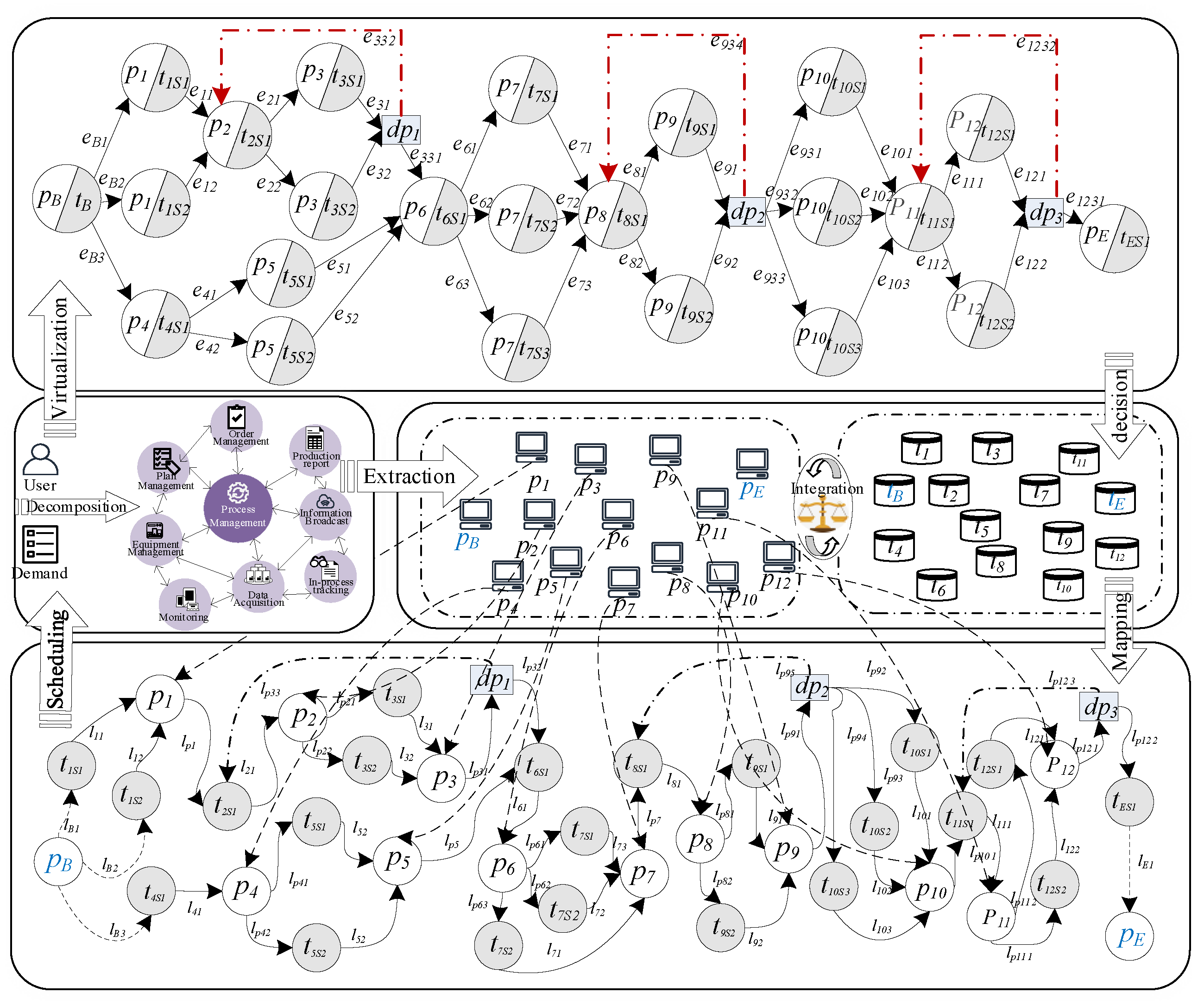
Figure 1. Non-linear production process work-flow model schematic.
Processes 11 01147 g001
Figure 2. Non-linear production process work-flow scheduling process.
Processes 11 01147 g002
Figure 3. VWFA algorithm virtual reconfiguration process.
Processes 11 01147 g003
Figure 4. Comparison of scheduling paths of different algorithms.
Processes 11 01147 g004
Figure 5. Impact of the number of process nodes on the algorithm VWFA.
Processes 11 01147 g005
Figure 6. Impact of deadlines on algorithms VWFA.
Processes 11 01147 g006
Table 1. Sheet metal manufacturing process node sets P and T.
NodeMeaningNodeMeaningNodeMeaning
p1Process classificationp2Programmingp3Machine adjustment
p4Profile processingp5Material calculationp6Material collection
p7Cuttingp8Bulk processingp9Adjustment
p10Process allocationp11Batch productionp12Warehouse
t1Category readyt2Program readyt3Machine ready
t4Processing readyt5Material preparationt6Distribution
t7Cutting readyt8Processing readyt9Adjustment ready
t10Allocation readyt11Production readyt12Storage ready
Table 2. Nodes and corresponding resource set.
NodeResources Set SNodeResources Set S
t1(2, 0.94, 0.2), (3, 0.96, 0.3)t2(1, 0.98, 1.2)
t3(1, 0.97, 0.3), (2, 0.99, 5)t4(1, 0.97,1.4)
t5(2, 0.97, 0.5), (3, 0.99, 0.7)t6(1, 0.99, 0.6)
t7(2, 0.90, 0.8), (3, 0.92, 1.0), (4, 0.95, 1.3)t8(15, 0.93, 19)
t9(2, 0.94, 0.7), (4, 0.98, 1.2)t10(3, 0.92, 0.3), (4, 0.95, 0.5), (6, 0.98, 0.6)
t11(10, 0.94, 14)t12(2, 0.96, 0.7), (3, 0.98, 1)
Table 3. Scheduling process and results of p′[1–3] under different deadlines.
DeadlineProcess
5Production quality ƒq = 0.931, production time ƒh = 6 and cost ƒc = 2; because ƒq < σ1q, execute correction processing, then ƒq = 0.931 + 0.931 × (1 − 0.931) = 0.995. ƒh = 6 + 1 = 7, ƒc = 2 + 0.5 = 2.5. Due to ƒh exceeds ME.H1, it does not meet the requirements and is discarded.
4The maximum production quality is equivalent to the maximum production accuracy of p1 when it begins at time 1, that ƒq = 0.913, production time ƒh = 5 and cost ƒc = 1.8; because ƒq < σ1q, execute correction processing, and ƒq = 0.913 + 0.913 × (1 − 0.913) = 0.992, ƒh = 5 + 1 = 6, ƒc = 1.8 + 0.5 = 2.3. Meets the requirements of dp1.
3The maximum production quality is equivalent to the maximum production accuracy of p1 when it begins at time 2, that ƒq = 0.894, production time ƒh = 5 and cost ƒc = 1.7; because ƒq < σ1q, execute correction processing, and ƒq(p1,2) = 0.894 + 0.894 × (1 − 0.894) = 0.989, ƒh = 5 + 1 = 6, ƒc = 1.7 + 0.5 = 2.2. Meets the requirements of dp1.
Table 4. Scheduling process and results of p′[6–9] under different deadlines.
DeadlineProcess
23Production quality ƒq = 0.857 and production time ƒh = 24; because ƒq < σ2q, execute correction processing, then ƒq = 0.857 + 0.857 × (1 − 0.857) = 0.980. ƒh = 24 + 2 = 26. Due to ƒh exceeds ME.H2, it does not meet the requirements and is discarded.
19The maximum production accuracy is equivalent to the maximum production accuracy of p1 when it begins at time 4, that ƒq = 0.796 and production time ƒh = 21; because ƒq < σ2q, execute correction processing, and ƒq = 0.796 + 0.796 × (1 − 0.796) = 0.958, ƒh = 21 + 2 = 23. Meets the requirements of dp2.
18The maximum production accuracy is equivalent to the maximum production accuracy of p1 when it begins at time 5, that ƒq = 0.779 and production time ƒh = 20; because ƒq < σ2q, execute correction processing, and ƒq = 0.779 + 0.779 × (1 − 0.779) = 0.951, ƒh = 20 + 2 = 22. Meets the requirements of dp2.
Table 5. Scheduling process and result of p′[10–12] under different deadlines.
DeadlineProcess
17Production quality ƒq = 0.903, production time ƒh = 21 and cost ƒc = 15.6; because ƒq < σ3q, execute correction processing, then ƒq = 0.903 + 0.903 × (1 − 0.903) = 0.990. ƒh = 21 + 2 = 23, ƒ’c = 18.6. Due to ƒh exceeds ME.H3, it does not meet the requirements and is discarded.
14The maximum production accuracy is equivalent to the maximum production accuracy of p1 when it begins at time 3, that ƒq = 0.986 ƒh = 18 and ƒc = 15.6; because ƒq < σ3q, execute correction processing, and ƒq = 0.860 + 0.860 × (1 − 0.860) = 0.980, ƒh = 18 + 2 = 20 and ƒ’c = 18.6. Meets the requirements of dp3.
13The maximum production accuracy is equivalent to the maximum production accuracy of p1 when it begins at time 4, that ƒq = 0.823 ƒh = 17 and ƒc = 15.6; because ƒq < σ3q, execute correction processing, and ƒq = 0.823 + 0.823 × (1 − 0.823) = 0.969, ƒh = 17 + 2 = 19, ƒ’c = 18.6. Meets the requirements of dp3.
Table 6. Local feasible solutions for each optimization section.
SegmentLocal SolutionPath
First segmentpath11pB/tBp1/t1S2p2/t2S1p3/t3S1, B0p4/t4S1p5/t5S1
path12pB/tBp1/t1S2p2/t2S1p3/t3S1, B0p4/t4S1p5/t5S2
path13pB/tBp1/t1S1p2/t2S1p3/t3S2, B0p4/t4S1p5/t5S1
path14pB/tBp1/t1S1p2/t2S1p3/t3S2, B0p4/t4S1p5/t5S2
Second segmentpath21p6/t6S1p7/t7S2p8/t3S1p9/t9S2
path22p6/t6S1p7/t7S3p8/t3S1p9/t9S1
path23p6/t6S1p7/t7S2p8/t3S1p9/t9S1
path24p6/t6S1p7/t7S1p8/t3S1p9/t9S2
Third segmentpath31p10/t10S2p11/t11S1p12/t12S2pE/tE
path32p10/t10S2p11/t11S1p12/t12S1pE/tE
path33p10/t10S1p11/t11S1p12/t12S1pE/tE
Table 7. Scheduling results of different algorithms.
Algorithm and ParameterCPMPAMVWFA
ƒqƒcƒhƒqƒcƒhƒqƒcƒh
First segment0.9295.050.9957.860.9896.26
Second segment0.95126.1220.96932.1280.97125.825
Third segment0.97018.0170.99018.6210.98618.519
Cumulative0.85750.1440.95558.5550.94750.550
Disclaimer/Publisher’s Note: The statements, opinions and data contained in all publications are solely those of the individual author(s) and contributor(s) and not of MDPI and/or the editor(s). MDPI and/or the editor(s) disclaim responsibility for any injury to people or property resulting from any ideas, methods, instructions or products referred to in the content.