Abstract
Although desalinations with renewables were introduced some time ago, conventional desalination units are still applied. Conventional desalinations account for 90% of desalinations worldwide. Yet, they have two significant issues: a high demand for energy and a high level of environmental contaminants. Such issues are studied and remedies are suggested in the current study. Varieties of biofuel blends in dual and ternary bases are investigated experimentally for indirect desalination. Results showed that ternary blends can introduce lower desalination potentials than fossil fuels by about 4–7%. The best ternary blends for the indirect desalination process are iBE, followed by niB, and finally EM. The EGT of iBE is greater than niB and EM by about 1.1 and 1.2%, respectively. Both n-butanol/iso-butanol–gasoline dual blends introduced an almost similar desalination potential as the ternary blends (e.g., lower desalination by about 4.4 and 4.7%). Nevertheless, bio-ethanol/bio-methanol–gasoline dual blends introduced greater desalination potentials than the fossil fuel by 3.2 and 3%, respectively. Regarding environmental issues, both ternary and dual blends introduced lower CO and UHC emissions than fossil fuels in varying degrees. M presented the lowest CO by about 30%, followed by EM by about 21%, and lastly E by about 20%, compared to G. However, the lowest UHC is presented by EM followed by nB and niB with rates of 18, 16.2, and 13.5%. Results also showed that the engine speed has a considerable effect on the desalination process and environment; low engine speed is recommended in the case of applying ternary blends, as well as dual n-butanol/iso-butanol–gasoline blends. Alternatively, in the case of applying bio-ethanol/bio-methanol–gasoline dual blends, moderate engine speed is preferable.
1. Introduction
Fresh water is one of the necessities for life, not only for humans, but also for animals and plants. Countries, due to such importance, try to obtain it using different methods. One of the methods currently applied worldwide is desalination. There are many techniques to desalinate salt water, such as membrane desalination and thermal desalination. Membrane desalination applies reverse osmosis (RO) technology, while thermal desalination applies multi-stage flash (MSF) and/or multi-effect distillation (MED). In membrane desalination, mechanical methods are applied for the filtration of salt from water through membranes. In thermal desalination methods, water is evaporated by using heat from different energy sources such as fossil fuels and/or renewable energies to separate salt from fresh water [1,2,3,4].
Renewable energies in the desalination process have some advantages, such as low emissions and renewable source (not depleted over time). One of the renewables currently used is solar desalination. Solar desalination has many advantages such as it is economically inexpensive and clean for the environment. However, it faces some challenges such as limited availability, as solar energy is only available during the day; consequently, desalination stops during night. This is in addition to the fact that some countries (quite a few) do not have access to the sun for some weeks or even months, which makes solar desalination unfeasible. This forced some countries into applying conventional desalination with fossil fuels instead. Currently, about 90% of desalination units worldwide are operated by fossil fuels [5,6]. However, such desalination units using fossil fuels are facing some challenges. First, is the high pollutant emissions [7,8]; second is the high energy demand; and third is the depletion of fossil fuels. Such challenges forced researchers to investigate alternative and renewable fuels [9,10].
The energy prerequisite for freshwater desalination units is considerable. Energy costs are about 40–60% of the total production costs in the desalination process [11]. MED and MSF desalination techniques, for example, need between 45 and 320 kWh/m3 of thermal energy and they need between 1.5 and 3 kWh/m3 electricity for pumping water and other product disposal [12,13]. There have been many efforts dedicated to improve the energy-efficiency of the process of desalination, through energy conservation and energy integration in desalination plants [14,15,16,17,18]. Several approaches have been taken to improve the energy footprint of desalination units. One solution for the high energy demand of desalination is by recovering lost heat from different devices and energy utilization. Researchers have worked in heat recovery from combustion engines as one of the auxiliary devices in desalination plants. However, from the review, very limited studies were found discussing the use of combustion engines in indirect desalination, as is summarized next. Shafieian and Khiadani [19] recovered the waste heat of submarine engines for desalination via both exhaust fumes and cooling water. The study concluded that while water is used to cool down the engine, hot water is cooled and the waste energy was recovered for desalination. Seyedkavoosi et al. [20] proposed a two-step system to recover the waste energy of a diesel engine within coolant water and exhaust fumes. Yang et al. [21] analyzed the heat recovery from engines and proposed a couple of temperature loops: a high temperature loop is powered by exhaust fumes and a low temperature loop is heated by the water jacket. Chintala et al. [22] reviewed the waste heat recovery from different engines via cooling water, exhaust fumes, and intake air. Lion et al. [23] focused on recovering waste heat from the oil system, exhaust fumes, intake air system, and the engine cooling system. Ouyang et al. [24] investigated a desalination method operated with waste heat recovery of marine engines. Lion et al. [25] proposed technologies, together with the related potentials, for waste heat recovery from combustion engines. Gude [26] applied desalination with the waste heat of marine combustion engines. Salimi and Amidpour [27] applied exhaust temperature gases of an internal combustion engine (ICE) as well as the water jacket warmness to produce steam for a multi-effect desalination process. Asadi et al. [28] applied a thermal desalination system driven by the waste heat of an engine. In summary of these early studies, one can recover the waste heat of a marine engine of capacity/power 7500 kW and recover energy to acquire distilled water volumes of about 1000 m3 per day. In small engines with capacities/powers between 33 and 55 kVA, one can obtain distilled water volumes between 1122 and 1817 m3 in a year by heat recovery.
The combustion engines used for desalination via the heat recovery process could be fueled with either fossil fuels or renewables. Since our aim is to replace fossil fuels, the use of renewable fuels in engines, especially in gasoline engines, is evaluated. Studies are carried out for bio-ethanol and bio-methanol blended in gasoline. Gong et al. [29] studied a spark ignition engine operated with bio-methanol and the results showed an increase in thermal efficiency, soot, and CO emissions. Elfasakhany [30,31] examined bio-methanol and bio-ethanol blended in gasoline and the results showed improvements in emissions and power of the engine compared to fossil fuels. Gong et al. [32,33] examined bio-methanol and hydrogen in a direct-injection engine and the results showed a decrease in CO2, UHC, and CO emissions, but with increasing soot emissions. Gong et al. [34] in another study examined bio-methanol/hydrogen dual blends in a spark-ignition engine and the results showed a decrease in soot emission. Zhen and Wang [35] applied an overview study of using bio-methanol as a fuel in internal combustion engines. The study showed a reduction in emissions with the bio-methanol fuel, compared to fossil fuels. Elfasakhany [36] investigated i-butanol/bio-methanol/gasoline and n-butanol/bio-ethanol/gasoline ternary blends. Results showed some benefits of using both ternary blended fuels. Elfasakhany [37] investigated bio-ethanol/bio-methanol/gasoline ternary blends and the results showed improvements in emissions and combustion of the blends. Elfasakhany [38] investigated n-butanol/i-butanol/gasoline ternary blends and the results endorsed biofuel blends more than conventional gasoline. Elfasakhany et al. [39] investigated the blend of n-butanol/bio-methanol/gasoline and the results established a reduction in engine combustion of the blends. Elfasakhany [40] applied bio-ethanol/i-butanol/gasoline blends and the results displayed an enhancement in engine pollutant emissions of the blends. Researchers in early studies [41,42,43,44,45] exposed a significant enhancement in engine performance/combustion and pollutant emissions of blended biofuels compared to conventional pure gasoline. Babu et al. [46] applied dual blends of 20% oil and 80% gasoline and showed an improved in fuel efficiency, in-cylinder pressure, and heat release rate. Lodi et al. [47] examined microalgae biofuel blends on engine performance characteristics during different engine operated conditions. The study reported an increase in indicated thermal efficiency but a decrease in indicated/brake mean effective pressure (IMEP/BMEP).
Researchers in recent studies intended to improve the economics of water desalination plants with innovative energy, efficiency, and inexpensive operation using energy recovery techniques, as highlighted earlier. In this work, different biofuel blends are applied as renewable fuel sources for desalination plants. Biofuels are investigated in terms of pollutant emissions and heat recovery from internal combustion engines. The biofuels are blended in ternary and dual products and compared with each other as well as with conventional gasoline for proposing the most promising one(s) for energy recovery and emissions in desalinations.
2. Experimental Setup and Procedure
The experiments of this research, as explained in this section, are carried out by investigating biofuel blends for energy recovery and emissions from an internal combustion engine. The engine is a small, four-stroke, single cylinder, gasoline/petrol fuel, and water-cooled type. Complete specifications of the engine are listed in Table 1. In addition to the engine, another device is applied to analyze and measure the amount/types of exhaust gases produced from engine. A gas analyzer of type Infralyt CL is selected for this study to measure carbon dioxide, carbon monoxide, and hydrocarbons in exhaust gases. The gas analyzer is connected via the exhaust pipe system of the engine and gives readings after about 10 min of starting up. The analyzer is light (less than 10 kg weight) and it is operated using 230 V (+10%/−15%) voltage, 50 +/−1 Hz frequency, and Max. 45 VA power consumption; complete specifications are listed in Table 1.

Table 1.
Gas analyzer and engine specifications.
The experimental set-up is carried out by starting up the exhaust gas analyzer and the engine for a while, and then the fuel is injected into the engine after blend preparation. The biofuel blends are prepared by mixing gasoline with different renewable biofuels to form seven different blended fuels. The seven blended fuels are prepared as discussed next. Firstly, gasoline is placed in a well-closed container/bottle, then iso-butanol is added to it at a rate of 7% by volume (the gasoline amount in the mixture is 93% by volume) and then they are well mixed and flipped over to form iso-butanol–gasoline blends (iB). Likewise, the rest of the fuel blends are prepared; in particular, 93% gasoline is mixed with 7% n-butanol (n-butanol–gasoline, nB); 93% gasoline is mixed with 7% bio-methanol (bio-methanol–gasoline, M); 93% gasoline is mixed with 7% bio-ethanol (bio-ethanol–gasoline, E). This is the preparation procedure for the dual blended types (four blends). In the case of mixing three different fuels (ternary blends), the same procedure is applied as follows: 93% gasoline is mixed with 3.5% bio-methanol and 3.5% bio-ethanol (bio-methanol–bio-ethanol–gasoline blends, EM); 93% gasoline is mixed with 3.5% iso-butanol and 3.5% bio-ethanol (iso-butanol–bio-ethanol–gasoline blends, iBE); 93% gasoline is mixed with 3.5% n-butanol and 3.5% iso-butanol (n-butanol–iso-butanol–gasoline blends, niB). In summary, seven different biofuel blends are prepared and considered, four of them in dual blend products and three in ternary blend products (the properties of different biofuels are shown in Table 2 [48,49,50,51]). After preparing all biofuel blends, they are injected into the engine one by one. It is important to clarify that only 7% by volume of renewable biofuel is mixed with gasoline (93% by volume). This low rate of biofuel in the blends is considered for a couple of reasons. Firstly, renewable biofuel is still economically expensive and therefore using a little of it may suffice. Secondly, the use of renewable fuel at high rates needs modification of engine specifications; however, using low rates can evade modifying engines and related costs in the automotive industry.
Table 2.
Fuel properties [48,49,50,51].
3. Results and Discussions
The results of different biofuel blends in dual and ternary products are presented and discussed. The discussions are limited here to comparisons between different blends rather than combustion and flame for such blends, as such discussions need a separate paper for each blend. A couple of result topics are presented and compared for each blend; in the first section, the effectiveness of each blend for the desalination process are introduced and, in the second section, the pollutant emissions are compared for such blends. All blends are examined under the same operating conditions to make the comparisons valuable and worthwhile. The effectiveness of desalination for each blend is presented in terms of exhaust gas temperature (EGT), while the pollutant emissions are evaluated for different blends via CO, UHC, and CO2 emissions. Comparing the results and findings with that of others is essential to support our outcomes and observations. Nevertheless, using our blends for desalination is not displayed in any previous studies. One can find a unique early study by the author of [52], which presented different blends for desalination.
Figure 1 shows the comparisons between exhaust gas temperatures (EGTs) for ternary blended fuels of bio-ethanol–bio-methanol–gasoline (EM), iso-butanol–bio-ethanol–gasoline (iBE), and n-butanol–iso-butanol–gasoline (niB); the conventional pure gasoline (G) is presented as a reference line in the figure. The comparisons, as shown in the figure, are presented at three different engine speeds (3500, 3000, and 2500 r/min); such speeds represent low, medium, and high engine speed conditions. As seen, all ternary blends showed lower EGTs than the gasoline fuel. The greatest EGT among all ternary blends is presented by iBE at all speeds. The lowest EGT (the poorest desalination) among all ternary blends is shown by EM, while niB showed moderate results between iBE and EM. In summary, the ternary blends provide lower recovered energy for desalination than the fossil gasoline by about 4–7%. Furthermore, as the engine speed increases, the EGT decreases, e.g., there is much lower recovered energy for desalination with increasing engine speeds.
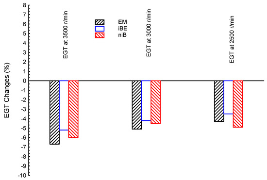
Figure 1.
Exhaust gas temperature (EGT) at three different engine speeds (3500, 3000, and 2500 r/min) for ternary blended fuels of bio-ethanol–bio-methanol–gasoline (EM), iso-butanol–bio-ethanol–gasoline (iBE), and n-butanol–iso-butanol–gasoline (niB); gasoline is the reference line.
Figure 2 shows the comparisons of EGTs for the ternary blended fuels (EM, iBE, and niB) in average testing within all engine speeds. As can be seen, the EGTs for EM, iBE, and niB are all lower than gasoline by about −5.5, −4.3, and −5.4%, respectively. In view of that, in order to use ternary blended biofuels for the indirect desalination process, the iBE is the best, followed by niB, and finally the EM. The EGT of iBE is greater than niB and EM by about 1.1 and 1.2%, respectively; while niB and EM are very close with little advantage for niB.
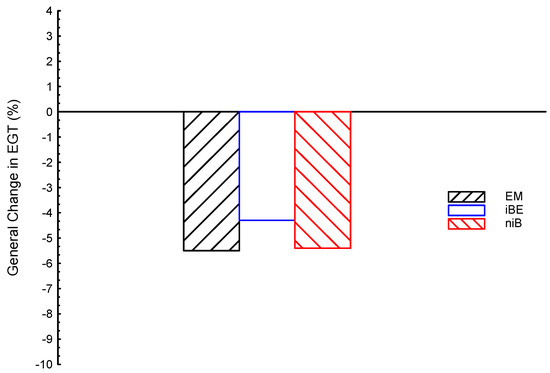
Figure 2.
Exhaust gas temperature (EGT) average for ternary blended fuels of bio-ethanol–bio-methanol–gasoline (EM), iso-butanol–bio-ethanol–gasoline (iBE), and n-butanol–iso-butanol–gasoline (niB); gasoline is the reference line.
Comparing the recovered energy for desalination using ternary blends against dual ones are carried out, as shown in Figure 3, Figure 4 and Figure 5. Each ternary blended biofuel is compared with the related dual ones to investigate the planned one(s) for desalination and, in turn, they/it are/is recommended for conventional desalination units. Figure 3 shows the exhaust gas temperature at three different engine speeds (3500, 3000, and 2500 r/min) for ternary blended bio-ethanol–bio-methanol–gasoline (EM), and dual bio-ethanol–gasoline (E) and bio-methanol–gasoline (M); gasoline is presented as a reference line in the figure. Both M and E showed greater EGTs than the G fuel at moderate- and high-speed conditions (3500 and 3000 r/min). However, EM showed a lower EGT than the G fuel at all speeds, as highlighted earlier. The E fuel showed greater EGT values by about 0.45, 3, and −1.5%, for high, medium, and low speeds, respectively, compared to G; while M showed greater EGT values by about 0.1, 3.2, and −0.7%, for high, medium, and low speeds, respectively, compared to G. Additionally, at high speed (3500 r/min), E presented the greatest EGT (it is greater than the M by 0.35%); however, at moderate speed (3000 r/min), the M blends showed the greatest EGT (M is greater than E by 0.2%). As well, both E and M dual blends showed much greater EGTs at moderate speeds than those values of the same blends in both low and high speed conditions. In conclusion, to apply E and M dual blends for indirect desalination, the engine speed should be under moderate conditions (~3000 r/min). Furthermore, at low engine speed, both dual blends (E and M) showed lower EGTs than the G fuel, and accordingly, such speed is not recommended. However, such low speed is preferred for the EM ternary blends; the EM ternary blends showed EGTs of about −6.7, −5.2, and −4.3% for high, medium, and low speeds, respectively, compared to G fuel. This means that the low engine speed is recommended for the desalination process while using ternary blends but this is contradicted in dual blends.
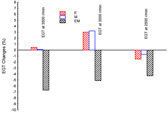
Figure 3.
Exhaust gas temperature (EGT) at three different engine speeds (3500, 3000, and 2500 r/min) for blended fuels of bio-ethanol–bio-methanol–gasoline (EM), bio-ethanol–gasoline (E), and bio-methanol–gasoline (M); gasoline is the reference line.
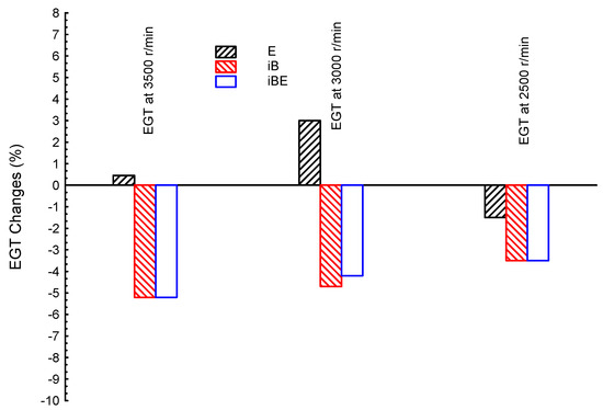
Figure 4.
Exhaust gas temperature (EGT) at three different engine speeds (3500, 3000, and 2500 r/min) for blended fuels of iso-butanol–bio-ethanol–gasoline (iBE), bio-ethanol–gasoline (E), and iso-butanol–gasoline (iB); gasoline is the reference line.
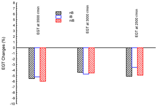
Figure 5.
Exhaust gas temperature (EGT) at three different engine speeds (3500, 3000, and 2500 r/min) for blended fuels of n-butanol–iso-butanol–gasoline (niB), iso-butanol–gasoline (iB), and n-butanol–gasoline (nB); gasoline is the reference line.
Figure 4 shows the comparisons of exhaust gas temperature at three different engine speeds (3500, 3000, and 2500 r/min) for ternary blended fuels of iso-butanol–bio-ethanol–gasoline (iBE), and dual blends bio-ethanol–gasoline (E) and iso-butanol–gasoline (iB); gasoline is presented as the reference line in the figure. It can be seen that both iB and iBE provide lower EGTs at all engine speeds, while E provides greater EGTs than the G fuel at a couple of speeds, as covered earlier. In particular, iB showed lower EGTs by −5.2, −4.7, and −3.5% for high, medium, and low speeds, respectively, compared to G fuel; while the iBE showed EGTs changes of −5.2, 4.2, and −3.5%, for high, medium, and low speeds, respectively, compared to G fuel. From such results, one can notice that both iB and iBE introduced very close results. Additionally, engine speed plays an important principle rule in the desalination process; medium speed is the best for E dual blends, while low speed is the best for iB and iBE blends.
Figure 5 shows the comparisons between exhaust gas temperatures for ternary blended fuel of n-butanol–iso-butanol–gasoline (niB), and dual iso-butanol–gasoline (iB) and n-butanol–gasoline (nB) at three different engine speeds (3500, 3000, and 2500 r/min); gasoline is the reference line in the figure. The results in numbers are as follows. The EGT difference for nB is about −5.5, −4.4, and −5.1%, for high, medium, and low speeds, respectively, compared to G fuel; the niB affected EGTs by −6, −4.5, and −4.9%, for high, medium, and low speeds, respectively, compared to G fuel; the iB showed lower EGT, as presented earlier, by −5.2, −4.7, and −3.5% for high, medium, and low speeds, respectively, compared to G fuel. In summary, iB, nB, and niB showed very close results and all blends have lower EGTs than the G fuel. In summary, the EGTs for iB, nB, and niB are in the range 4–6% lower than the G fuel.
In overview comparisons of EGTs for the dual and ternary blends, the best EGTs are introduced by E and M dual blends. However, the ternary EM, niB, and iBE blends, in addition to the dual nB and iB blends, are all lower than the G fuel. The reasons of such results may be attributed to the following details. The properties of biofuels are extremely different, as shown in Table 2. The greatest biofuel oxygen content is introduced by bio-methanol (50%), followed by bio-ethanol (35%), and lastly by both b-butanol and iso-butanol with 21.5% for both. That may cause more complete combustion, e.g., greater EGT, for E and M dual blends (even greater than G fuel). However, although both iB and nB contain oxygen in their chemical structures, they showed lower EGTs than the G fuel (G contains zero oxygen in the fuel structure, as shown in Table 2). This may be attributed to how the dual blended fuels (iB and nB) are introduced into the engine without any tuning or adjustments. The engine working conditions (such as compression ratio, spark timing, and fuel injection time) are all adjusted for gasoline fuel and, accordingly, the engine is compatible with gasoline properties. The properties of both iB and nB require many more tuning conditions than the E and M. Furthermore, E and M showed greater EGTs than the gasoline fuel, although the engine is not adjusted for such blends due to their much greater oxygen contents; this means that in the case of tuning the engine for M and E, such blends would present much higher EGT results. Regarding the ternary blends (EM, niB, and iBE), the EGTs relative to G are small due to requiring considerable engine tuning for such blends; additionally, blending of three different biofuels for ternary blended issues may make them subject to a separation problem, e.g., one biofuel may separate from another. This may be the genuine reason of lower EGTs relative to G for EM ternary blends, although such blends contain a high oxygen content.
One of the very big problems in conventional desalination units is the emissions. Pollutant emissions are investigated and compared for the proposed biofuel blends. Figure 6 shows CO emissions at three different engine speeds (3500, 3000, and 2500 r/min) for ternary blended bio-ethanol–bio-methanol–gasoline (EM), iso-butanol–bio-ethanol–gasoline (iBE), and n-butanol–iso-butanol–gasoline (niB); gasoline is the reference line in the figure. The lowest emission of CO is introduced by EM, followed by iBE, and lastly niB at all speeds. All ternary blends introduced lower CO emissions than the gasoline fuel (except for niB at 3500 r/min). Additionally, the CO emissions generally decreased as the engine speed increased. Hence, high speed is recommended at using ternary blends for achieving low CO emissions.
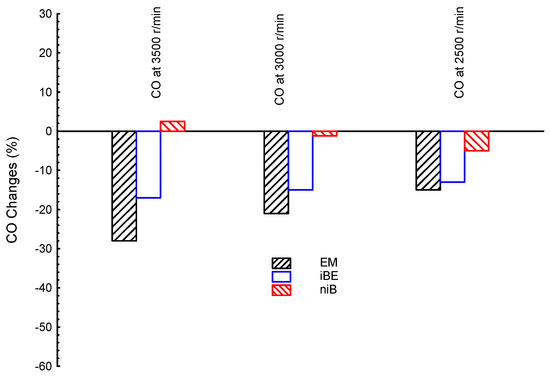
Figure 6.
CO emissions at three different engine speeds (3500, 3000, and 2500 r/min) for ternary blended fuels of bio-ethanol–bio-methanol–gasoline (EM), iso-butanol–bio-ethanol–gasoline (iBE), and n-butanol–iso-butanol–gasoline (niB); gasoline is the reference line.
The unburned hydrocarbons (UHC) are also investigated in the study. Figure 7 shows the UHC emissions at three different engine speeds (3500, 3000, and 2500 r/min) for ternary blended fuels of EM, iBE, and niB, as well as conventional gasoline as a reference line. It can be seen that the EM showed the lowest values at all speeds followed by iBE, and finally niB, similarly to the CO results. Additionally, all ternary blends presented lower UHC emissions than the G fuel.
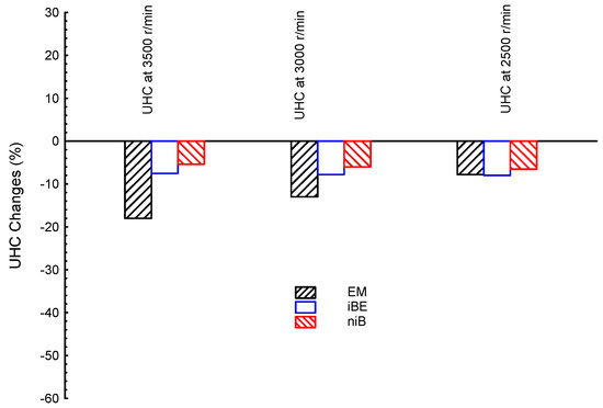
Figure 7.
UHC emission at three different engine speeds (3500, 3000, and 2500 r/min) for ternary blended fuels of bio-ethanol–bio-methanol–gasoline (EM), iso-butanol–bio-ethanol–gasoline (iBE), and n-butanol–iso-butanol–gasoline (niB); gasoline is the reference line.
Figure 8 shows CO2 emissions for the ternary blended fuels (EM, iBE, and niB) and gasoline as the reference line at three different engine speeds (3500, 3000, and 2500 r/min). As shown, the most CO2 is introduced by EM at all speeds, where the emission levels are higher than the G fuel; while both iBE and niB showed lower CO2 levels than the G fuel. The lowest CO2 is introduced by niB among all ternary blends at all engine speeds, as shown in Figure 8. The CO2 emissions for different blends are reproduced as averages for an easier comparison point of view, as presented subsequently.
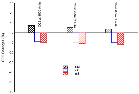
Figure 8.
CO2 emission at three different engine speeds (3500, 3000, and 2500 r/min) for ternary blended fuels of bio-ethanol–bio-methanol–gasoline (EM), iso-butanol–bio-ethanol–gasoline (iBE), and n-butanol–iso-butanol–gasoline (niB); gasoline is the reference line.
In addition to the results at different speeds (as shown in Figure 6, Figure 7 and Figure 8), all emissions (CO, UHC, and CO2) are introduced as averages, to be easily compared. Figure 9 shows CO, CO2, and UHC emissions averages for ternary blended fuels (EM, iBE, niB) and G as a reference line. The EM showed emission levels changed by −21, −18, and 6.3%, compared to G; the iBE showed CO, UHC, and CO2 values of −14, −14, and −14%, compared to G; the niB showed emission values of about −5, −13.5, and −18%, for CO, UHC, and CO2, respectively, compared to G. In summary, the lowest CO is introduced by EM where it is lower than those of iBE and niB by about 7 and 16%, respectively. The iBE showed a moderate level of CO emission between EM and niB blends; while the greatest CO is introduced by niB (but it is still lower than the G fuel). The UHC emission results are almost similar to CO emissions; the EM showed the lowest CO and it is lower than both iBE and niB blends by about 4 and 4.5%, respectively. Regarding CO2, the lowest is introduced by niB, followed by iBE, and lastly by EM blends. The niB is lower than iBE and EM by about 24.3 and 4 %, respectively. In conclusion, the EM ternary blend is recommended among all ternary blends for offering the best/lowest emissions (CO and UHC); iBE introduced moderate emissions between EM and niB for all emissions. Please note that CO2 is not considered as emission by various studies.
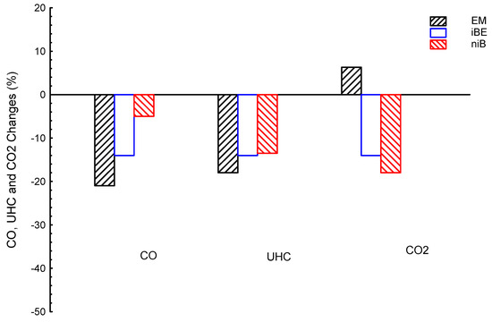
Figure 9.
CO, CO2, and UHC emissions averages for ternary blended fuels of bio-ethanol–bio-methanol–gasoline (EM), iso-butanol–bio-ethanol–gasoline (iBE), and n-butanol–iso-butanol–gasoline (niB); gasoline is the reference line.
Comparing the emissions of ternary blends with dual ones is carried out based on averages. Figure 10 shows CO, CO2, and UHC emissions averages for use of bio-ethanol–bio-methanol–gasoline (EM) ternary blended fuel and dual bio-ethanol–gasoline (E) and bio-methanol–gasoline (M); gasoline is the reference line. As shown, M presented the lowest CO by about −30%, followed by EM by about −21%, and lastly E by about −20%, compared to G. The UHC results showed the lowest value by EM, followed by M, and finally E; in numbers, EM, M, and E are about −18, −12.8, and −10%, respectively, compared to G. The CO2 results showed greater values than the G by about 6.3, 10, and 4.6% for EM, M, and E, respectively, compared to G. In summary, CO emissions of M are the lowest; they is lower than those of EM and E by about 9 and 10%, respectively. The UHC emissions of EM are the lowest; they are lower than M and E by about 5.2 and 8%, respectively. Additionally, both ternary (EM) and dual blends (E and M) introduced the same trends for all emissions, e.g., CO and UHC are lower and CO2 is higher than the G fuel.
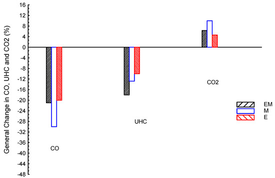
Figure 10.
CO, CO2, and UHC emissions averages for ternary blended fuels of bio-ethanol–bio-methanol–gasoline (EM), bio-ethanol–gasoline (E), and bio-methanol–gasoline (M); gasoline is the reference line.
Figure 11 shows CO, CO2, and UHC emissions averages for n-butanol–iso-butanol–gasoline (niB) ternary blended fuel and dual n-butanol–gasoline (nB) and iso-butanol–gasoline (iB); gasoline is the reference line. iB presented the lowest CO by about −11.6%, followed by nB by about −10%, and lastly niB by about −5%, compared to G. The UHC results showed the lowest value by nB, followed by niB, and finally iB; in numbers, nB, niB, and iB are about −16.2, −13.5, and −6.8%, respectively, compared to G. The CO2 results showed lower values than the G by about −36, −35, and −18% for iB, nB, and niB, respectively, compared to G. In summary, CO emissions of iB are the lowest; they is lower than those of nB and niB by about 1.6 and 6.6%, respectively. The UHC emissions of nB are the lowest; they are lower than the niB and iB by about 2.7 and 9.4%, respectively. To finish, both ternary (niB) and dual blends (iB and nB) introduced the same trend for all emissions, e.g., CO, UHC, and CO2 are all lower than the G fuel.
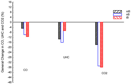
Figure 11.
CO, CO2, and UHC emissions averages for blended fuels of n-butanol–iso-butanol–gasoline (niB), n-butanol–gasoline (nB), and iso-butanol–gasoline (iB); gasoline is the reference line.
Figure 12 shows CO, CO2, and UHC emissions averages for iso-butanol–bio-ethanol–gasoline (iBE) ternary blended fuel and dual iso-butanol–gasoline (iB) and bio-ethanol–gasoline (E); gasoline is the reference line. E presented the lowest CO by about −20%, followed by iBE by about −14%, and lastly iB by about −11.6%, compared to G. The UHC results showed the lowest value by iBE, followed by E, and finally iB; in numbers, iBE, E, and iB are about −14, −10, and −6.8%, respectively, compared to G. The CO2 results showed lower values than the G by about −36 and −14 for iB and iBE, respectively, while E showed a higher value by 4.6%, compared to G. In summary, CO emissions of E are the lowest; they is lower than those of iBE and iB by about 6 and 8.4%, respectively. The UHC emissions of iBE are the lowest; they are lower than the E and iB by about 4 and 7.2%, respectively.
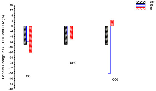
Figure 12.
CO, CO2, and UHC emissions averages for blended fuels of iso-butanol–bio-ethanol–gasoline (iBE), iso-butanol–gasoline (iB), and bio-ethanol–gasoline (E); gasoline is the reference line.
In overview comparisons for the different blends, all ternary blends can introduce lower desalination potentials (lower EGT) than the G fuel. Additionally, dual blends iB and nB can introduce similar desalination potentials as ternary blends (lower EGT). However, E and M dual blends can introduce greater desalination potentials than the G. The engine speed has a considerable effect on the desalination process; in the case of applying ternary blends, as well as dual iB and nB blends, low engine speed is recommended. However, in the case of applying dual E and M blends, moderate engine speed is preferable. Regarding emissions, all ternary and dual blends introduced lower CO and UHC emissions than conventional gasoline at different levels and, accordingly, they all are recommended (but one blend may be more desirable than another). The emissions are also very related to engine speeds, and as such, speed should be defined carefully.
4. Conclusions
Different biofuel blends in dual and ternary products are proposed and compared for desalination and environmental issues. Three blended fuels in ternary products and four blended in dual products are introduced and investigated. They are compared to each other as well as with conventional gasoline (G) at different engine speeds (low, moderate, and high). Results showed that ternary blends introduced lower desalinations than the G fuel at all speeds by about 4–7%. The greatest desalination among all ternary blends is presented by iBE (iso-butanol–bio-ethanol), while the lowest is introduced by EM (bio-ethanol–bio-methanol) at all speeds. The EGTs for EM, iBE, and niB are all lower than gasoline by about 5.5, 4.3, and 5.4%, respectively. Comparing desalinations between ternary/dual blends and gasoline showed that iB (iso-butanol), nB (n-butanol), and niB provided very close results and they are all lower than the G fuel in the range 4.5%; additionally, the E and M blends are superior compared to the G fuel by 3 and 3.2%, respectively. Regarding emissions, all ternary and dual blends introduced lower environmental emissions (CO and UHC) than the conventional gasoline. M presented the lowest CO (30%), followed by EM (21%), and lastly E (20%), compared to G. However, the lowest UHC emissions were afforded by EM (lower than G by 18%). The engine speed showed a considerable effect on environmental impact as well as the desalination process; low engine speed is recommended in the case of applying ternary blends as well as dual iB and nB blends; however, moderate engine speed is preferable in the case of applying dual E and M blends.
Funding
This research received no external funding.
Acknowledgments
This work was supported by Taif University researchers supporting project number (TURSP-2020/40), Taif University, Taif, Saudi Arabia.
Conflicts of Interest
The authors declare no conflict of interest.
References
- Møllebjerg, A.; Zarebska, A.; Nielsen, H.B.; Hansen, L.B.S.; Sørensen, S.R.; Seredynska-Sobecka, B.; Villacorte, L.O.; Gori, K.; Palmén, L.G.; Meyer, R.L. Novel high-throughput screening platform identifies enzymes to tackle biofouling on reverse osmosis membranes. Desalination 2023, 554, 116485. [Google Scholar] [CrossRef]
- Elfasakhany, A. Performance assessment and productivity of a simple-type solar still integrated with nanocomposite energy storage system. Appl. Energy 2016, 183, 399–407. [Google Scholar] [CrossRef]
- Alsehli, M.; Saleh, B.; Elfasakhany, A.; Aly, A.A.; Bassuoni, M.M. Experimental study of a novel solar multi-effect distillation unit using alternate storage tanks. J. Water Reuse Desalination 2020, 10, 120–132. [Google Scholar] [CrossRef]
- Lawal, D.U.; Qasem, N.A. Humidification-dehumidification desalination systems driven by thermal-based renewable and low-grade energy sources: A critical review. Renew. Sustain. Energy Rev. 2020, 125, 109817. [Google Scholar] [CrossRef]
- Ali, M.T.; Fath, H.E.S.; Armstrong, P.R. A comprehensive techno-economical review of indirect solar desalination. Renew. Sustain. Energy Rev. 2011, 15, 4187–4199. [Google Scholar] [CrossRef]
- Shatat, M.; Riffat, S.B. Water desalination technologies utilizing conventional and renewable energy sources. Int. J. Low-Carbon Technol. 2012, 9, 1–19. [Google Scholar] [CrossRef]
- Jabari, F.; Nazari-heris, M.; Mohammadi-ivatloo, B.; Asadi, S.; Abapour, M. A solar dish Stirling engine combined humidification-dehumidification desalination cycle for cleaner production of cool, pure water, and power in hot and humid regions. Sustain. Energy Technol. Assess. 2020, 37, 100642. [Google Scholar] [CrossRef]
- Hassan, H.; Yousef, M.S. An assessment of energy, exergy and CO2 emissions of a solar desalination system under hot climate conditions. Process. Saf. Environ. Prot. 2020, 145, 157–171. [Google Scholar] [CrossRef]
- Ghazi, Z.M.; Rizvi, S.W.F.; Shahid, W.M.; Abdulhameed, A.M.; Saleem, H.; Zaidi, S.J. An overview of water desalination systems integrated with renewable energy sources. Desalination 2022, 542, 116063. [Google Scholar] [CrossRef]
- Brendel, L.P.; Shah, V.M.; Groll, E.A.; Braun, J.E. A methodology for analyzing renewable energy opportunities for desalination and its application to Aruba. Desalination 2020, 493, 114613. [Google Scholar] [CrossRef]
- Zarzo, D.; Prats, D. Desalination and energy consumption. What can we expect in the near future? Desalination 2018, 427, 1–9. [Google Scholar] [CrossRef]
- Gude, V.G.; Fthenakis, V. Energy efficiency and renewable energy utilization in desalination systems. Prog. Energy 2020, 2, 022003. [Google Scholar] [CrossRef]
- Shahzad, M.W.; Ng, K.C.; Thu, K.; Saha, B.B.; Chun, W.G. Multi effect desalination and adsorption desalination (MEDAD): A hybrid desalination method. Appl. Therm. Eng. 2014, 72, 289–297. [Google Scholar] [CrossRef]
- Brogioli, D.; Yip, N.Y. Energy efficiency analysis of membrane distillation for thermally regenerative salinity gradient power technologies. Desalination 2022, 531, 115694. [Google Scholar] [CrossRef]
- Tian, S.; Guo, L.; Gu, Y.; Ju, S.; Xu, L. Energy transfer and efficiency analysis of microwave flash evaporation with tap water as medium. Desalination 2021, 511, 115095. [Google Scholar] [CrossRef]
- Shin, Y.-U.; Lim, J.; Boo, C.; Hong, S. Improving the feasibility and applicability of flow-electrode capacitive deionization (FCDI): Review of process optimization and energy efficiency. Desalination 2021, 502, 114930. [Google Scholar] [CrossRef]
- Cao, H.; Mao, Y.; Wang, W.; Gao, Y.; Zhang, M.; Zhao, X.; Sun, J.; Song, Z. Thermal-exergy efficiency trade-off optimization of pressure retarded membrane distillation based on TOPSIS model. Desalination 2021, 523, 115446. [Google Scholar] [CrossRef]
- Liu, T.; Lyv, J.; Xu, Y.; Zheng, C.; Liu, Y.; Fu, R.; Liang, L.; Wu, J.; Zhang, Z. Graphene-based woven filter membrane with excellent strength and efficiency for water desalination. Desalination 2022, 533, 115775. [Google Scholar] [CrossRef]
- Shafieian, A.; Khiadani, M. A multipurpose desalination, cooling, and air-conditioning system powered by waste heat recovery from diesel exhaust fumes and cooling water. Case Stud. Therm. Eng. 2020, 21, 100702. [Google Scholar] [CrossRef]
- Seyedkavoosi, S.; Javan, S.; Kota, K. Exergy-based optimization of an organic Rankine cycle (ORC) for waste heat recovery from an internal combustion engine (ICE). Appl. Therm. Eng. 2017, 126, 447–457. [Google Scholar] [CrossRef]
- Yang, F.; Cho, H.; Zhang, H.; Zhang, J. Thermoeconomic multi-objective optimization of a dual loop organic Rankine cycle (ORC) for CNG engine waste heat recovery. Appl. Energy 2017, 205, 1100–1118. [Google Scholar] [CrossRef]
- Chintala, V.; Kumar, S.; Pandey, J.K. A technical review on waste heat recovery from compression ignition engines using organic Rankine cycle. Renew. Sustain. Energy Rev. 2018, 81, 493–509. [Google Scholar] [CrossRef]
- Lion, S.; Michos, C.N.; Vlaskos, I.; Rouaud, C.; Taccani, R. A review of waste heat recovery and Organic Rankine Cycles (ORC) in on-off highway vehicle Heavy Duty Diesel Engine applications. Renew. Sustain. Energy Rev. 2017, 79, 691–708. [Google Scholar] [CrossRef]
- Ouyang, T.; Su, Z.; Gao, B.; Pan, M.; Chen, N.; Huang, H. Design and modeling of marine diesel engine multistage waste heat recovery system integrated with flue-gas desulfurization. Energy Convers. Manag. 2019, 196, 1353–1368. [Google Scholar] [CrossRef]
- Lion, S.; Vlaskos, I.; Taccani, R. A review of emissions reduction technologies for low and medium speed marine Diesel engines and their potential for waste heat recovery. Energy Convers. Manag. 2020, 207, 112553. [Google Scholar] [CrossRef]
- Gude, V.G. Thermal desalination of ballast water using onboard waste heat in marine industry. Int. J. Energy Res. 2019, 43, 6026–6037. [Google Scholar] [CrossRef]
- Salimi, M.; Amidpour, M. Modeling, simulation, parametric study and economic assessment of reciprocating internal combustion engine integrated with multi-effect desalination unit. Energy Convers. Manag. 2017, 138, 299–311. [Google Scholar] [CrossRef]
- Asadi, A.; Meratizaman, M.; Hosseinjani, A.A. Feasibility study of small-scale gas engine integrated with innovative net-zero water desiccant cooling system and single-effect thermal desalination unit. Int. J. Refrig. 2020, 119, 276–293. [Google Scholar] [CrossRef]
- Gong, C.; Yi, L.; Zhang, Z.; Sun, J.; Liu, F. Assessment of ultra-lean burn characteristics for a stratified-charge direct-injection spark-ignition methanol engine under different high compression ratios. Appl. Energy 2020, 261, 114478. [Google Scholar] [CrossRef]
- Elfasakhany, A. Comparisons of Using Ternary and Dual Gasoline–Alcohol Blends in Performance and Releases of SI Engines. Arab. J. Sci. Eng. 2021, 46, 7495–7508. [Google Scholar] [CrossRef]
- Elfasakhany, A. State of Art of Using Biofuels in Spark Ignition Engines. Energies 2021, 14, 779. [Google Scholar] [CrossRef]
- Gong, C.; Li, Z.; Yi, L.; Liu, F. Comparative study on combustion and emissions between methanol port-injection engine and methanol direct-injection engine with H2-enriched port-injection under lean-burn conditions. Energy Convers. Manag. 2019, 200, 112096. [Google Scholar] [CrossRef]
- Gong, C.; Li, Z.; Chen, Y.; Liu, J.; Liu, F.; Han, Y. Influence of ignition timing on combustion and emissions of a spark-ignition methanol engine with added hydrogen under lean-burn conditions. Fuel 2018, 235, 227–238. [Google Scholar] [CrossRef]
- Gong, C.; Li, Z.; Yi, L.; Huang, K.; Liu, F. Research on the performance of a hydrogen/methanol dual-injection assisted spark-ignition engine using late-injection strategy for methanol. Fuel 2020, 260, 116403. [Google Scholar] [CrossRef]
- Zhen, X.; Wang, Y. An overview of methanol as an internal combustion engine fuel. Renew. Sustain. Energy Rev. 2015, 52, 477–493. [Google Scholar] [CrossRef]
- Elfasakhany, A. Exhaust emissions and performance of ternary iso-butanol–bio-methanol–gasoline and n-butanol–bio-ethanol–gasoline fuel blends in spark-ignition engines: Assessment and comparison. Energy 2018, 158, 830–844. [Google Scholar] [CrossRef]
- Elfasakhany, A. Investigations on the effects of ethanol–methanol–gasoline blends in a spark–ignition engine: Performance and emissions analysis. Eng. Sci. Technol. Int. J. 2015, 18, 713–719. [Google Scholar] [CrossRef]
- Elfasakhany, A. Experimental study of dual n-butanol and iso-butanol additives on spark-ignition engine performance and emissions. Fuel 2016, 163, 166–174. [Google Scholar] [CrossRef]
- Elfasakhany, A.; Mahrous, A.F. Performance and emissions assessment of n-butanol–methanol–gasoline blends as a fuel in spark–ignition engines. Alex. Eng. J. 2016, 55, 3015–3024. [Google Scholar] [CrossRef]
- Elfasakhany, A. Engine performance evaluation and pollutant emissions analysis using ternary bio-ethanol–iso-butanol–gasoline blends in gasoline engines. J. Clean. Prod. 2016, 139, 1057–1067. [Google Scholar] [CrossRef]
- Elfasakhany, A. Experimental study on emissions and performance of an internal combustion engine fueled with gasoline and gasoline/n-butanol blends. Energy Convers. Manag. 2014, 88, 277–283. [Google Scholar] [CrossRef]
- Elfasakhany, A. Performance and emissions analysis on using acetone–gasoline fuel blends in spark-ignition engine. Eng. Sci. Technol. Int. J. 2016, 19, 1224–1232. [Google Scholar] [CrossRef]
- Elfasakhany, A. Performance and emissions of spark-ignition engine using ethanol–methanol–gasoline, n-butanol–iso-butanol–gasoline and iso-butanol–ethanol–gasoline blends: A comparative study. Eng. Sci. Technol. 2016, 19, 2053–2059. [Google Scholar] [CrossRef]
- Elfasakhany, A. Investigations on performance and pollutant emissions of spark-ignition engines fueled with n-butanol–, iso-butanol–, ethanol–, methanol–, and acetone–gasoline blends: A comparative study. Renew. Sustain. Energy Rev. 2017, 71, 404–413. [Google Scholar] [CrossRef]
- Elfasakhany, A. Gasoline engine fueled with bioethanol-bio-acetone-gasoline blends: Performance and emissions exploration. Fuel 2020, 274, 117825. [Google Scholar] [CrossRef]
- Babu, A.M.; Saravanan, C.; Vikneswaran, M.; Geo, V.E.; Sasikala, J.; Josephin, J.F.; Das, D. Analysis of performance, emission, combustion and endoscopic visualization of micro-arc oxidation piston coated SI engine fuelled with low carbon biofuel blends. Fuel 2020, 285, 119189. [Google Scholar] [CrossRef]
- Lodi, F.; Zare, A.; Arora, P.; Stevanovic, S.; Ristovski, Z.; Brown, R.J.; Bodisco, T. Engine performance characteristics using microalgae derived dioctyl phthalate biofuel during cold, preheated and hot engine operation. Fuel 2023, 344, 128162. [Google Scholar] [CrossRef]
- Elfasakhany, A. Experimental investigation on SI engine using gasoline and a hybrid iso-butanol/gasoline fuel. Energy Convers. Manag. 2015, 95, 398–405. [Google Scholar] [CrossRef]
- Elfasakhany, A. Biofuels in Automobiles: Advantages and Disadvantages: A Review. Curr. Altern. Energy 2019, 3, 27–33. [Google Scholar] [CrossRef]
- Elfasakhany, A. Alcohols as Fuels in Spark Ignition Engines: Second Blended Generation; Lambert Academic Publishing: Saarbrücken, Germany, 2017; ISBN 978-3-659-97691-9. [Google Scholar]
- Elfasakhany, A. Benefits and Drawbacks on the Use Biofuels in Spark Ignition Engines; LAP LAMBERT Academic Publishing: Beau Bassin, Mauritius, 2017; ISBN 978-620-2-05720-2. [Google Scholar]
- Elfasakhany, A. Dual and Ternary Biofuel Blends for Desalination Process: Emissions and Heat Recovered Assessment. Energies 2020, 14, 61. [Google Scholar] [CrossRef]
Disclaimer/Publisher’s Note: The statements, opinions and data contained in all publications are solely those of the individual author(s) and contributor(s) and not of MDPI and/or the editor(s). MDPI and/or the editor(s) disclaim responsibility for any injury to people or property resulting from any ideas, methods, instructions or products referred to in the content. |
© 2023 by the author. Licensee MDPI, Basel, Switzerland. This article is an open access article distributed under the terms and conditions of the Creative Commons Attribution (CC BY) license (https://creativecommons.org/licenses/by/4.0/).