Decision Support Tool for the Optimal Sizing of Solar Irrigation Systems

Abstract

Solar photovoltaic (PV) irrigation is increasingly used in agriculture, driven by its low operation cost and virtually zero emissions, providing electricity access in rural areas. However, the high investment cost requires an optimal design. The objective of this work was to develop a user-friendly tool to optimally size a PV generator that satisfies crop irrigation needs under local constrictions. The ODSIS (Optimal Design of Solar Irrigation System) tool, was organized in three calculation modules, preceded by two complements, which determine the daily crop irrigation needs and power demand of the pumping system. Then, the first module sizes the PV plant, considering a multiplication factor, and provides the PV production potential throughout each day of the season. The second and third modules evaluate the total investment cost and equivalent greenhouse gas emissions avoided by comparison with traditional energy sources. This tool was applied to a case study in Senegal for which a multiplication factor of 1.4 was obtained for the optimal PV plant size. Between 22% to 64% of the investment cost corresponded to the PV pumping system, depending on the irrigation technique. The use of PV energy in the case study would represent an annual economic saving for the farmer after 5 to 8 years of payback period, avoiding the emission of between 29.8 and 37.9 tCO₂eq/year for the case study area.

1. Introduction

Population growth, particularly in developing regions such as sub-Saharan Africa (SSA), is leading to an intensification of irrigated areas and, therefore, increased energy consumption, resulting in higher greenhouse gas (GHG) emissions [1]. Photovoltaic (PV) irrigation is seen as a promising low-GHG emissions alternative to the use of traditional energy sources (fossil fuels and the electricity grid) [2]. PVs offers economic and environmental savings during the operational life cycle of the installation [3], providing energy supply to remote areas without electricity grid access. For this reason, developments in PV irrigation systems and the integration of environmental considerations with technical and economic aspects should be translated to the conditions of smallholder irrigation, a thriving sector in SSA [4,5].

However, there are two important issues regarding the use of solar irrigation systems: the high investment cost and the risk of overexploitation of water resources, especially in rural areas in African countries. According to Mérida García et al. [6], the investment cost of PV technology is generally higher than the corresponding costs of traditional energy sources (diesel generator and electricity grid). The second main constraint is related to the risk of overexploitation of water resources due to the virtually zero operating cost of solar energy. For these reasons, sizing methodologies considering the optimal size of the generators to meet the specific crop water demand for each case are required.

The design and dimensioning of PV energy systems for irrigation have been the subjects of numerous studies. Most investigations focused on technical aspects, determining the PV plant size as a function of the crop water requirements and the irrigation network power needs [7,8]. López–Luque et al. [9] proposed a simulation model for standalone PV irrigation systems to determine the optimal energy output capacity with the highest economic profitability. Rezk et al. [10] added a battery bank to the PV system to maintain a continuous power supply, and Kazem et al. [11] included economic considerations in the design. None of these works included environmental aspects, something evaluated by Mérida García et al. [6] in an economic and environmental analysis of PV irrigation in on-grid and off-grid scenarios.

To make the proposed design techniques and optimization models more accessible, user-friendly tools have started to emerge. However, few tools have been developed in this context. Some authors have developed Excel-based tools for solar pumping system sizing. The Solar Water Pumping Worksheet by Jenkins and Bolivar-Mendoza [12] and the Toolbox on Solar Powered Irrigation Systems (SPIS), implemented by the German Agency for International Cooperation [13], are some examples. Both tools base the PV sizing methodology on daily average values of irrigation water requirements and irradiation for the day with the highest water demand, the former being applicable to any location, with the second one restricted to a specific area (New Mexico, Arizona, Colorado, Utah, Nevada, Wyoming, and Montana).

This work presents a user-friendly tool, called ODSIS, for the optimal size of PV irrigation systems. This tool is organized in three modules: PV generator sizing tool, economic assessment tool, and environmental evaluation tool. The tool is developed as a package of Microsoft Excel spreadsheets that can be used for any region of the world. Unlike most other available tools, ODSIS bases the PV system sizing on the daily performance of the system by checking the satisfaction of the daily energy in irrigation demand during the whole irrigation season. Furthermore, ODSIS calculates the potential capital cost of the system and provides the amount of GHG emission savings during the operation of the system compared to conventional energy sources. These results facilitate a comparative analysis of different design options. Finally, the operation of the ODSIS tool is illustrated by a case study of small-scale irrigation in northern Niayes, Senegal.

2. ODSIS Tool Description

ODSIS tool consists of three main modules, further defined below:

-

PV generator sizing module.

-

Economic assessment module

-

Environmental assessment module

The PV sizing module calculates the required PV nominal power to satisfy the crop irrigation requirements during the whole irrigation season (see

Table A1. Irrigation season for the different crops.

Crop	Jan.	Feb.	Mar.	Apr.	May	Jun.	Jul.	Aug.	Sept.	Oct.	Nov.	Dec.
Onion (Orient F1)
Onion (Sonsa)
Turnip
Cabbage
Tomato
Pepper
Chili
Eggplant

Irrigation season is in gray.

), considering the all crops used (Figure A1). This is determined considering the power demands of the irrigation system and a multiplication factor, as further explained below. Once the PV array is sized, the tool checks whether daily irrigation time can be satisfied during a whole irrigation season based on hourly irradiance data for an average year. In those cases in which one pump operates to irrigate more than one plot (the plots are called sectors), the irrigation scheduling considers that the sector with the highest demand irrigates during the hours with the highest PV power production.

If the simulation of a whole year shows that there are some days in the season in which the system cannot satisfy the total irrigation requirements, the nominal power of the PV installation is increased by increasing the value of the multiplication factor. The operation of the system is then recalculated for the entire irrigation season. When necessary, a reservoir can be integrated into the system to compensate the irrigation time to meet the irrigation water requirements, allowing the reduction of the multiplication factor. This reservoir can be used as a “support” system, to reduce the PV installation size (as explained below). In addition, there is also the option of directly filling the reservoir and irrigating by gravity from the reservoir, avoiding direct-pump irrigation, if preferred by the user. This option also allows improving the irrigator well-being by reducing exposure during peak irradiance hours. When a reservoir is included, the pump is simply sized according to the power requirements for pumping to fill the reservoir. The reservoir is always considered to be placed at the highest area of the plot to then allow gravity to determine the irrigation flow.

Once the PV nominal power is determined, the investment cost is assessed for the different components of the PV irrigation system (pump and PV array components, pipes, and emitters).

Finally, the environmental impact module estimates the potential GHG emissions avoided with the use of PV energy instead of a diesel generator or the electricity grid, when applicable.

ODSIS consists of a set of MS Excel sheets (Figure 1):

-

Read me;

-

Geometric factor;

-

Beam and diffuse irradiance;

-

Irradiance on collector plane;

-

Photovoltaic power controller;

-

Power transferred to the pump;

-

Net Power in the peak period;

-

Summary;

-

Investment;

-

Grid electricity emission factor;

-

GHG emission.

The “Read me” sheet explains the meaning of all the symbols, providing an over-view of the formulas used for the calculation of the pump and PV generator size. The following six sheets comprise the PV generator sizing module. The optimal size deter-mined for the PV array is presented in the “Summary” sheet. Finally, the “Investment” sheet presents the economic results, and the last two sheets (grid electricity emission factor and GHG emission) show the results related to the environmental impact estimation. The user must enter data and may observe specific results in all these sheets except in the “Read me” and “Summary” sheets. The MS Excel Book contains 365 additional sheets with a day-by-day checking of the hourly fulfilment of irrigation water requirements.

ODSIS has two complementary tools that need to be run before any other calculations can be made. These complements are Excel spreadsheets that provide: (i) the daily water requirements for each crop and plot/sector (Complement 1), and (ii) the minimum pumping power requirements of the irrigation plot/sectors (Complement 2).

Complement 1 estimates the daily irrigation time for each plot/sector. It is composed of five sheets: guideline; crop information; crop coefficient and evapotranspiration; net irrigation requirements; and gross irrigation requirement (GIR) for drip, sprinkler and manual irrigation. The user fills in this tool data about crop type, crop coefficients, length of the different phenological stages of the crop (see

Table A2. Duration of crop stages and crop coefficient values for the case study crops.

Crops	Growing Period (Days)				Kc Value
	Initial	Development	Mid-Season	Late-Season	Initial	Mid-Season	Late-Season
Onion	20	35	90	45	0.5	1.05	0.85
Turnip	20	30	30	15	0.6	1.1	0.9
Cabbage	20	30	30	15	0.45	1.05	0.9
Tomato	30	40	40	25	0.45	1.15	0.8
Pepper	30	35	40	20	0.35	1.05	0.9
Chili	30	35	40	20	0.35	1.05	0.9
Eggplant	30	40	40	20	0.45	1.15	0.8

Sources: [19,28,29].

), daily reference evapotranspiration and rainfall, the crop area, the sowing date, and the average irrigation efficiency for each irrigation technique.

Complement 2 determines the pump flow rate and pressure head. This complement is organized in eight sheets: guideline; gross irrigation requirement; pump flow rate; adjustment factor for drip irrigation (ratio of the friction loss in a lateral with the number of sprinkler outlets on the lateral having equal spacings and discharges); design for drip irrigation; Fn for sprinkler irrigation; design for sprinkler irrigation; and design for manual irrigation. The user manually fills in this tool with the irrigation water requirements previously determined (Complement 1), and some data related to the irrigation network (length, diameter, and head losses of pipes) and information related to the emitters (spacing, number, flow rate, and operating pressure) are added.

3. Calculation Procedure in the ODSIS Tool and Its Complements

3.1. Method of Calculating the PV Generator Sizing Module

The peak power of the PV generator (PP, in W) is sized according to the most power-demanding sector of the farm, being then adjusted by means of a multiplication factor to mitigate the effect of the solar energy production curve. This multiplication factor ranges between one and two. An iterative process of simulation of the operation of the system for the whole irrigation season can be made by the user, allowing for the adjustment of the multiplication factor to increase its value (and so the peak power of the PV generator) when the irrigation is not fully satisfied (Figure 2). The system’s operation is simulated by estimating the PV power production potential of the plant throughout the day, based on Equation (1) [9,14]:

$${\mathrm{P}}_{\mathrm{PVn}\mathrm{t}}=\frac{{\mathrm{I}}_{\mathrm{nt}}}{{\mathrm{I}}_{\mathrm{stc}}}\times \mathrm{PP}\times \left[1-\mathrm{b}\left({\mathrm{T}}_{\mathrm{cell}}-{\mathrm{T}}_{\mathrm{stc}}\right)\right]$$

(1)

where P_PV is the available instantaneous PV power (W); I is the irradiance on the collector plane (W/m²); n is the day; t is the time; I_stc is the irradiance under standard conditions (1000 W/m²); PP is the PV peak power (W); b is the performance decay coefficient due to the rising temperature of the module cells, equal to 0.004 °C⁻¹ for silicon cells; T_cell is the PV cell temperature (°C); and T_stc is the PV cell temperature under standard conditions (25 °C).

The energy generated by solar panels can be maximized in terms of their usage [15]. As a result, the PV pumping system must be sized taking into account several aspects. Firstly, the output power generated from the solar cell may be low in efficiency because the amount of electricity delivered by solar panels is directly proportional to the solar radiation input received by the panel collectors [15]. Therefore, proper knowledge of the system design and choice of suitable design parameters are key in achieving cost-effectiveness and efficient performance of any given system. Thus, according to Sharma et al. [16], ambient irradiance and temperature, PV and array geometry, load data and sizing algorithm, etc., are required to size the solar pumping system. On the other hand, Cuadros et al. [7] and Kumar et al. [17] consider that the pumped water flow rate, the incident solar radiation, and the PV array size are all important.

The irradiance on the collector plane is computed using Equation (2):

$${\mathrm{I}}_{\mathrm{n}\mathrm{t}}={\mathrm{R}}_{\mathrm{b}}\times {\mathrm{I}}_{\mathrm{bn}\mathrm{t}}+\frac{1+\cos \mathsf{\phi }}{2}\times {\mathrm{I}}_{\mathrm{dn}\mathrm{t}}+\partial \times \frac{1-\cos \mathsf{\phi }}{2}\times \left[{\mathrm{I}}_{\mathrm{bn}\mathrm{t}}+{\mathrm{I}}_{\mathrm{dn}\mathrm{t}}\right]$$

(2)

where R_b is the geometric factor, I_b is the beam irradiation on the tilted plane to that on a horizontal surface (W/m²), I_d is the diffuse irradiance (W/m²), $\partial$ is the albedo, and φ is the tilt angle of the modules (degree). R_b is calculated using Equation (3) [18]:

$${\mathrm{R}}_{\mathrm{b}}=\frac{\cos \mathsf{\theta }}{\cos \mathsf{\theta }\mathrm{z}}$$

(3)

where ϴ is the angle of incidence, and ϴ_z is the zenith angle.

The ${\mathrm{T}}_{\mathrm{cell}}$ is computed using Equation (4) in which T_a represents the air temperature and S the slope coefficient, equal to 0.003 °C/W/m² for silicon cells.

$${\mathrm{T}}_{\mathrm{cell}}={\mathrm{T}}_{\mathrm{a}}+\mathrm{S}\times {\mathrm{I}}_{\mathrm{n}\mathrm{t}}$$

(4)

Once the hourly average PV power potential production for each day of the irrigation season is determined (for an average year), the tool checks whether the available irrigation hours (those with available power equal to or higher than the power demand of the plots/sectors) are sufficient to satisfy the total irrigation time required. Therefore, the estimation of the power transferred to the pump considers the inverter efficiency, which is equal to 95% in this study.

3.1.1. Method of Calculating the Irrigation Water Requirements

The gross irrigation requirement (GIR, in mm) is calculated in Complement 1 based on the net irrigation requirement (NIR, in mm) of the crop and the efficiency of the irrigation system (E_a), following Equation (5):

$$\mathrm{GIR}=\frac{\mathrm{N}\mathrm{I}\mathrm{R}}{{\mathrm{E}}_{\mathrm{a}}}$$

(5)

NIR is determined daily, considering the crop irrigation needs, based on the difference between the crop evapotranspiration (ET_c) and the effective rainfall (R_eff). ET_c (Equation (6)) is calculated based on the FAO method [19] in which ET_o is the reference evapotranspiration (mm) calculated using the FAO–Penman–Monteith equation [19], and K_c is the crop coefficient, which varies with the crop phenological stage:

$${\mathrm{ET}}_{\mathrm{c}}={\mathrm{ET}}_{\mathrm{O}}\times {\mathrm{K}}_{\mathrm{c}}$$

(6)

The K_c values during the development and late season stages are determined using Equations (7) and (8), respectively:

$${\mathrm{K}}_{\mathrm{c}\mathrm{dev}}={\mathrm{K}}_{\mathrm{c}\mathrm{ini}}+\left[\frac{\mathrm{m}-{\mathrm{L}}_{\mathrm{ini}}}{{\mathrm{L}}_{\mathrm{dev}}}\right]\left({\mathrm{K}}_{\mathrm{c}\mathrm{mid}}-{\mathrm{K}}_{\mathrm{c}\mathrm{ini}}\right)$$

(7)

$${\mathrm{K}}_{\mathrm{c}\mathrm{lat}}={\mathrm{K}}_{\mathrm{c}\mathrm{mid}}+\left[\frac{\mathrm{m}-{\mathrm{L}}_{\mathrm{mid}}}{{\mathrm{L}}_{\mathrm{lat}}}\right]\left({\mathrm{K}}_{\mathrm{c}\mathrm{lat}}-{\mathrm{K}}_{\mathrm{c}\mathrm{mid}}\right)$$

(8)

where m is the day of the crop cycle; ini, dev, mid, and lat refer to the initial, development, mid-season, and late-season stages, respectively; and L is the duration of each stage (days).

R_eff is estimated following the methodology proposed by FAO [19]:

$${\mathrm{R}}_{\mathrm{eff}}=0.6\mathrm{R}-10\mathrm{if}\mathrm{R}<70\mathrm{mm}/\mathrm{month}$$

(9)

$${\mathrm{R}}_{\mathrm{eff}}=0.8\mathrm{R}-24\mathrm{if}\mathrm{R}>70\mathrm{mm}/\mathrm{month}$$

(10)

3.1.2. Method of Calculating the Power Required by the Pump

The power requirements for the irrigation of the different plots/sectors are determined based on the head pressure and flow requirements, following Equation (11):

$${\mathrm{P}}_{\min \mathrm{i}}=\frac{\mathsf{\rho }\times {\mathrm{Q}}_{\mathrm{i}}\times {\mathrm{H}}_{\mathrm{i}}}{{\mathsf{\eta }}_{\mathrm{p}}}$$

(11)

where P_min is the power requirements to irrigate plot/sector i (W), ρ is the specific weight of the water (N/m³), Q is the flow rate (m³/s), H is the required pressure head (m), and η_p is the efficiency of the pump.

For drip and sprinkler irrigation systems, the flow rate was calculated based on the emitter flow rate and the number of emitters. For manual irrigation, farmers use buckets to take water from several small tanks installed at different levels, filled with water pumped from the boreholes. In this case, the flow rate is determined based on the number of basins that the farmer will irrigate together.

The pressure requirements are calculated section by section following the methodology described in Sarr et al. [20], using Equation (12):

$$\mathrm{H}\mathrm{i}={\mathrm{H}}_{\mathrm{di}}+\Delta \mathrm{Z}+{\mathrm{h}}_{\mathrm{f}1\mathrm{i}}+{\mathrm{h}}_{\mathrm{f}2\mathrm{i}}+{\mathrm{H}}_{\mathrm{emi}}$$

(12)

where H (m) is the pressure head; H_d (m) is the dynamic height; ∆Z (m) is the difference in elevation between the water source and the most unfavorable supply inlet; h_f1 (m) is the head loss from the pump to the most unfavorable supply inlet; and h_f2 (m) and H_em (m) are the head losses from the inlet to the most unfavorable emitter, and the pressure required at the emitter, respectively, both used for drip and sprinkler irrigation techniques.

3.2. Economic Assessment Module

The ODSIS tool integrates a module for the estimation of the investment cost of the PV irrigation system. The investment cost calculations include the cost of the pump and the solar panels (including installation) and the cost associated to the irrigation system, including drippers or sprinklers, pipes, and filters. In this module, a partial calculation is possible for those farmers who already have an irrigation system and only need to replace the energy source. The total investment cost (TIC) is determined as a function of the unit price of the selected equipment (P, in EUR) and the number of units (i.e., number of PV panels, number of valves, etc.) or length (i.e., total pipe length for a specific diameter) (q) of the equipment and materials needed, as shown in Equation (13):

$$\mathrm{TIC}={\displaystyle \sum }\mathrm{q}\left(\mathrm{P}\right)$$

(13)

A list of component prices, the result of a survey conducted with suppliers of solar irrigation pumps and irrigation systems in the Niayes area (Senegal) in 2019 [21], is available in the tool. However, the user can update this information to suit any case study. This list includes prices for different pumps’ characteristics and various brands. In the case of the PV panels, a nominal power range between 80 W to 300 W is covered. In addition, the prices of electric cables, drippers (900 µ and 600 µ), sprinklers, PVC or galvanized pipes with diameters in the range 32 mm to 160 mm, filters, and small accessories, are available. The user should select the equipment required and the number of units needed to obtain the total investment cost.

3.3. Environmental Impacts Assessment Module

The environmental impact module evaluates the potential GHG emissions avoided when the use of a diesel generator or the electricity grid is replaced by the PV system. These estimations were based on the total energy demand of the irrigation system, considering a specific emission factor associated to each energy source (diesel generator or the electricity mix for each country).

When comparing the use of PV energy with the use of a diesel generator, the equivalent GHG emissions avoided were estimated considering the potential fuel consumption for one irrigation season. This fuel consumption was determined based on the diesel generator size required and irrigation time, accounting for the impact burden associated with the climate change impact category for this fuel, based on the Ecoinvent database [22]. However, for the use of the electricity grid, the energy demand in each farm was calculated based on the power requirements and the irrigation time for each sector. In this case, the varying electricity mix structure for each country was considered, using a specific GHG emission factor for each country.

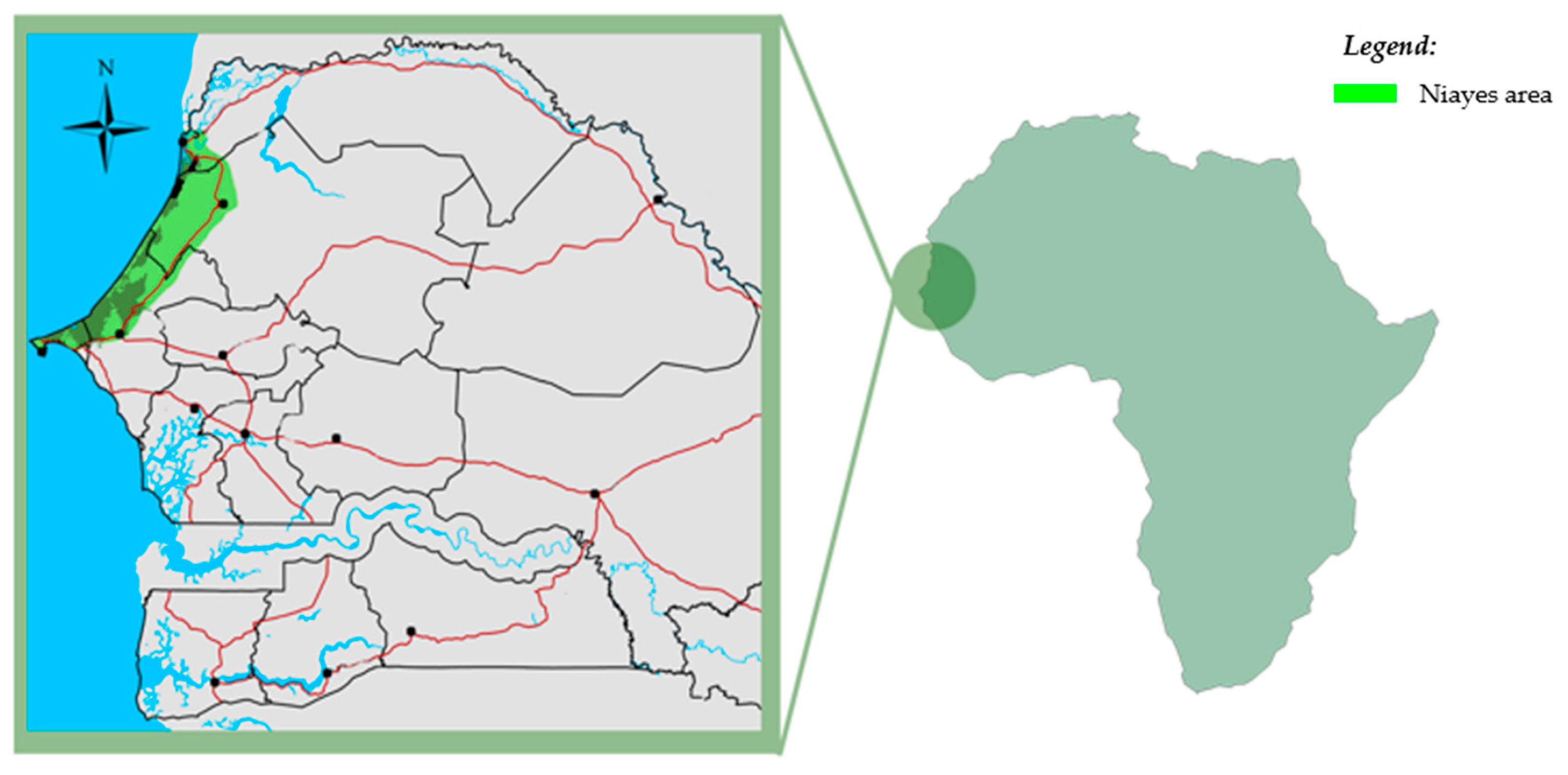
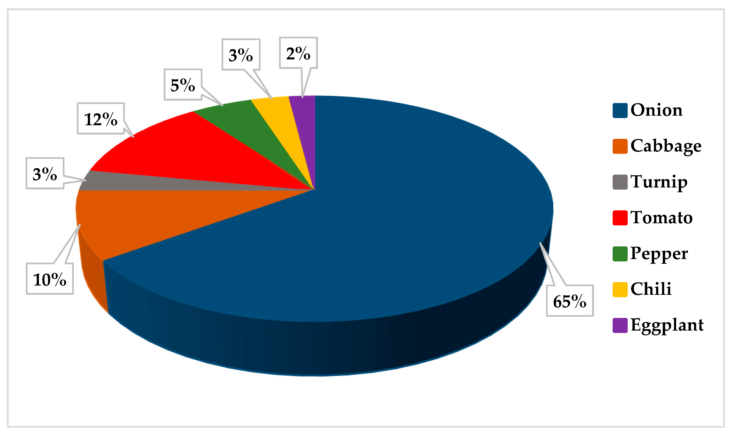
4. Application of the ODSIS Tool in the Niayes Area in Senegal

4.1. Study Area

Nguethiouro was selected as a case study. This area is located in the Gandiolais region, at the southern end of the Senegal Delta (Figure 3). It is an integral part of the Niayes area, a coastal fringe, which extends from Dakar to Saint-Louis over a length of 180 km, with a width varying from 5 to 30 km [23].

The Nguethiouro area is geographically localized between 16°28′30″ and 16°24′05″ W and 15°50′20″ and 15°56′10″ N, with Sahelian climate. It is characterized by an average annual rainfall of about 300 mm. Average annual temperatures range between 23.7 °C and 25 °C, while the highest average monthly temperatures range from 27.5 °C to 28.1 °C, occurring during the rainy season [24]. The mean daily global irradiance varies between 15 MJ/m² and 23 MJ/m². The highest value can achieve 28 MJ/m² and may occur in August. Figure 4 shows the average variation of the daily mean values throughout the year for air temperature, global irradiance, and precipitation in the Nguethiouro lowland for the period 1990 to 2020.

The Nguethiouro lowland is composed of 15 plots (ranging from 0.05 ha to 1.91 ha). The irrigation water is exclusively extracted from the groundwater, with the water table depth varying between 3 to 8.9 m, depending on the plot. In this lowland, most of the farmers use individual pumps. Only a small part of them uses the pumps grouped because of family ties. Therefore, in this case study, the pumps are sized individually for most of the plots, and in groups (Group 1 and Group 2) for 4 of them. Both groups integrate two plots each, with Plots 3 and 5 included in Group 1 and Plots 9 and 12 included in Group 2. In these cases, irrigation is organized by rotation, and plots are called sectors.

It is important to note that agriculture in the Nguethiouro lowland is characterized by a partial cultivation of the land, so each farmer only cultivates about half of the plot area at the same time. This is mainly due to the lack of financial means to cover the fuel cost, the lack of water from the wells, and the varying soil quality. For these reasons, Plots 10, 13, and 15 are not cultivated by their owners. Figure 5 shows the cultivated areas.

4.2. Results and Discussion of the Application to the Case Study

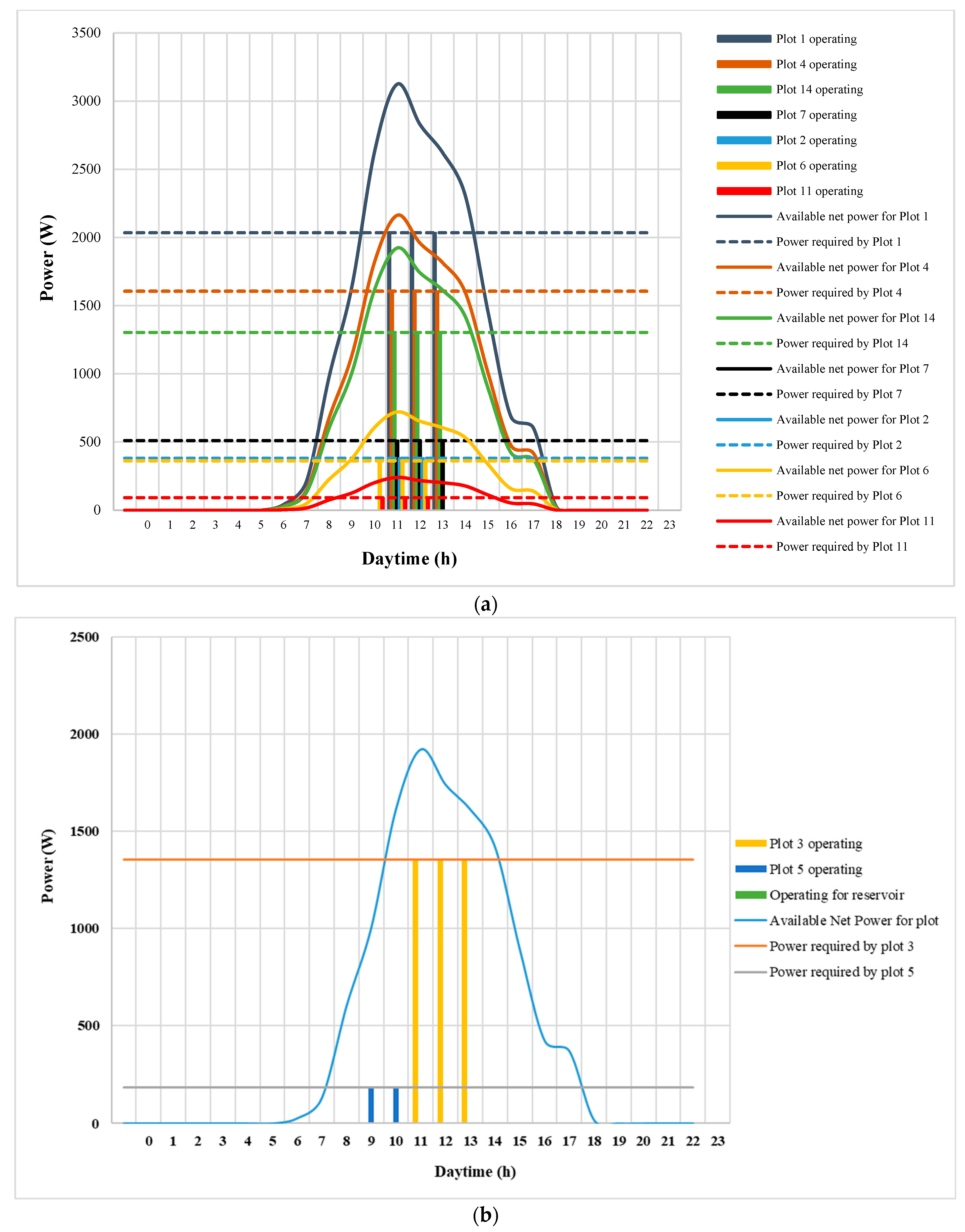
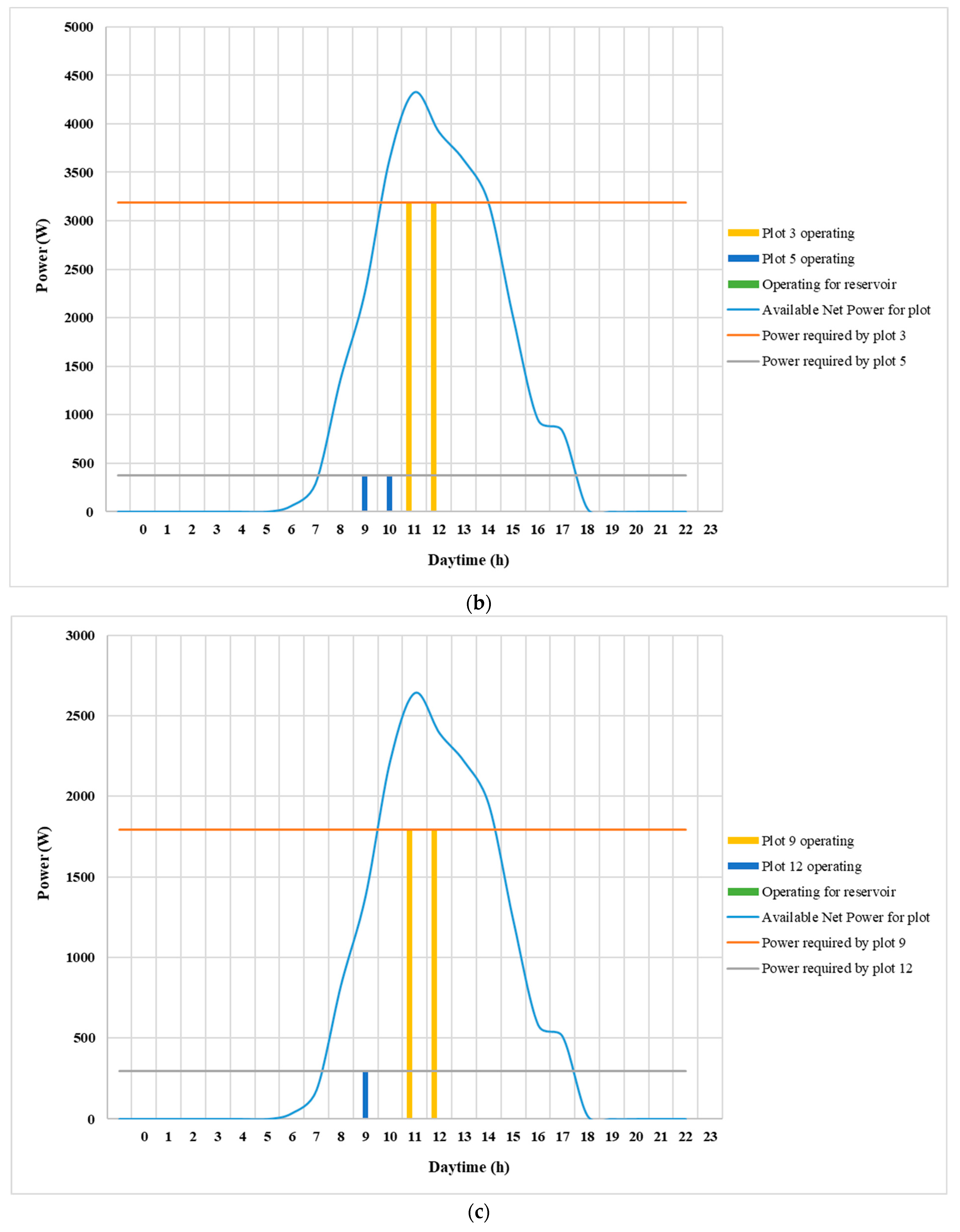
4.2.1. Power and Energy Requirements for Irrigation

Irrigation water requirements varied depending on the irrigation system and crop (

Table 1. Power requirements for manual and drip irrigation techniques.

Plot/Sector (Group)	Irrigated Area (ha)	Irrigation Water Requirements Used (m3)	Irrigation Time (h)	Flow Rate Q (m3/h)	Pressure Head H (m)	Minimum Power Required P min (W)	Energy (kWh)
		Manual irrigation system
1	0.96	54.27	2.6	20.95	24.95	2035	1551
2	0.19	10.80	2.3	4.78	20.55	382	242
3 (1)	0.57	32.11	2.2	14.33	24.25	1353	858
4	0.71	40.06	2.2	17.84	23.13	1606	1020
5 (1)	0.08	4.26	2.0	2.1	22.57	185	117
6	0.15	8.24	2.2	3.77	24.68	362	230
7	0.24	13.64	2.3	6.03	21.79	511	325
8	0.16	8.81	2.2	4.02	21.44	336	214
9 (2)	0.38	21.31	2.2	9.55	23.07	858	545
11	0.06	3.41	2.3	1.51	15.68	92	58
12 (2)	0.04	2.27	2.3	1.1	15.76	62	39
14	0.48	27.28	2.3	12.06	27.78	1304	828
		Drip irrigation system
1	0.96	51.25	1.5	34.2	38.79	5164	2598
2	0.19	10.20	1.7	6.0	35.72	834	468
3 (1)	0.57	30.32	1.5	20.3	40.3	3185	1481
4	0.71	37.84	1.4	26.5	37.5	3869	1846
5 (1)	0.08	4.03	1.5	2.6	36.9	373	206
6	0.15	7.78	1.4	5.7	38.97	865	395
7	0.24	12.88	1.3	9.7	36.4	1376	530
8	0.16	8.32	1.5	5.5	35.9	769	398
9 (2)	0.38	20.13	1.7	11.8	38.98	1791	1112
11	0.06	3.22	0.8	4.1	30.74	491	192
12 (2)	0.04	2.15	0.8	2.6	29.5	299	109
14	0.48	25.76	1.6	15.7	40.17	2455	1355

). Water requirements were higher when using manual irrigation systems, obtaining the lowest results for drip irrigation systems. This was due to the varying efficiencies for the different irrigation techniques for which an average value of 85% and 90% was applied for manual and drip irrigation, respectively [25].

Energy refers to the PV energy requirements for a whole irrigation season.

The irrigation water requirements varied between 2.27 m³ and 54.27 m³ for areas that varied between 0.04 ha and 0.96 ha with daily irrigation time between 2 h and 3 h in the case of manual irrigation. For drip irrigation, the irrigation water requirements were lower, varying between 2.15 m³ and 51.25 m³, for the same range of areas with daily irrigation time varying between 1 h and 2 h. Currently, manual irrigation is used by 93.3% of farmers in the Nguethiouro lowland. However, water scarcity is driving the transition to drip irrigation, which offers a more efficient use of water.

Table 1 shows the flow rate, pressure head, and power required by the pumping system to irrigate each plot when using manual and drip irrigation techniques. Regarding the groups, the pumps are sized based on the most power demanding sector. Thus, for Group 1 (Plots 3 and 5), the pump was sized to satisfy the power requirements of Plot 3. Then, the irrigation schedule was organized by rotation, ensuring the satisfaction of the energy required by the total sectors (2) that compound the group.

Results show that the pump flow rate varied between 1.1 m³/h and 20.95 m³/h and between 2.6 m³/h and 34.2 m³/h for manual and drip irrigation techniques, respectively, which supposed a difference between 63 and 136%.

Head pressure requirements also varied according to the irrigation technique used, the covered area, the topography of the plots, the water table, and the drawdown. In this study, a constant drawdown of 10 m was assumed according to Niang [26] and Seck et al. [27]. Therefore, the pressure head requirements ranged from 15.68 m to 27.78 m for manual irrigation (which only accounts for the water elevation from the borehole to the reservoir), while the application of water through a pressurized network (drip irrigation) increased these values up to 88%.

Power requirements of the pump varied between 1.55 kW/ha (Plot 12) and 2.12 kW/ha (Plot 1) for manual irrigation, while drip irrigation required between 5.38 kW/ha (Plot 12) and 7.48 kW/ha (Plot 1). In this case study, the power requirements were influenced significantly by topography due to the interdunal depression that characterizes this area. These power requirements represented annual energy demands that varied between 0.98 kWh/ha (Plot 12) and 1.62 kWh/ha (Plot 1) for the manual irrigation system, respectively. For the drip irrigation system, the annual energy requirements were equal to 2.7 kWh/ha (for both Plot 12 and Plot 1). The power required by the pump in the case of drip irrigation was much higher than that required for manual irrigation since the drippers need some pressure for their operation. However, low pressure was required in the case of manual irrigation to pump water from the source to the small ponds. In addition, the water sources in the Niayes area are located inside the agricultural plots, which reduces the operating power of the pumps used for irrigation.

In addition, comparing the results of ODSIS with other previous available tools, for a plot of 0.96 ha, the Toolbox for SPIS gave a system power of 13 kW, which is much higher than the power offered by ODSIS for drip irrigation. This calculation is carried out considering a static level of 8.5 m and a drop of 19 m. The primary pipe and the secondary pipes are all evaluated at a length of 98 m.

4.2.2. PV Generator Sizing

The most restrictive day in the irrigation season for the case study analyzed, considered in an early stage of the sizing, corresponded to 4 July, with water requirements of 5.68 mm and 5.37 mm for manual and drip irrigation techniques, respectively.

Figure 6 and Figure 7 show the irrigation scheduling for the peak period (4 July) for the different plots and sectors when the power provided by the PV plant is high enough to satisfy the irrigation time for each plot (or sector) during the whole irrigation season. This was possible for a multiplication factor of 1.4, so the power requirements for pumping were increased up to 3 kW for the most demanding plot, also considering the efficiency of the inverter.

Figure 6 and Figure 7 show that the operation time of the PV irrigation system varied between 1 and 3 h for the different plot/sectors during 4 July. The hourly and seasonal variability regarding the renewable energy generation represents a key issue faced by PV energy-based irrigation systems. In the case study analyzed, the best results when using manual irrigation system were obtained for a multiplication factor of 1.4. This multiplication factor allowed meeting the daily irrigation water requirements during all the irrigation season. In those cases in which the pumps were used for more than 1 plot (Groups 1 and 2), the irrigation started from 8 or 9 a.m. with the operation of the sector with the lowest power demand (0.18 kW), starting the irrigation of the most demanding sector from 11 a.m. when the PV power reached the corresponding power threshold (1.35 kW). In addition, it was observed that when the multiplication factor used was 1.1, the water requirements are only met for 115 days in the year. Therefore, it may have problems irrigating for the remaining days of the year.

Figure 6 and Figure 7 show the differences in the irrigation scheduling when comparing manual irrigation with drip irrigation. Figure 7a shows that drip irrigation started at 11 a.m., finishing at 1 p.m. (2 h) for the plots that irrigate individually, as a higher power was required to operate compared to manual irrigation. In the case of Group 1 and Group 2, the results show that the most power-demanding plot of each group (Plot 3 and 9, respectively) started irrigating at 11 a.m., as in the case of the manual irrigation system, while the plots with lower power requirements were activated earlier in the morning (at 9 a.m.). In the case of the drip irrigation technique, the multiplication factor also equaled 1.4.

Thus, the smaller plot that needs less pressure to operate the irrigation system irrigates during the hours of minimum sunlight, and the larger plot irrigates during the hours of maximum sunlight to meet the irrigation water requirements. This is very beneficial, allowing us to reduce the size of the PV array because irrigation is performed by rotation.

However, it should be noted that the data used for the case study are not measured data. The data used are estimated from databases, which may have an impact on the results. However, these data can be used because they are close to reality. However, it would be interesting for a user of the tool to use the measured data when possible.

4.2.3. Economic and Environmental Assessment

The total investment cost varied according to different components, such as the pump characteristics and brand, the nominal power of the PV panel selected, the diameter of the pipes, the type of dripper and filter used, etc. The results for the case study showed that generally, the total investment cost decreased for higher nominal power of the PV panels.

The pump type was chosen for each case based of its characteristics (flow and head pressure required) and price. Regarding the panels, the nominal power was selected based on the cost and the availability in the market.

Table 2. Total investment cost of PV irrigation when using manual and drip irrigation techniques for an area of 0.96 ha.

Nominal Power of the PV Panel (W)	Manual Irrigation (EUR)	Drip Irrigation (600 µ) (E)
80	5595	11,021
100	5659	11,162
120	5511	10,834
150	5416	10,657
250	5151	9736
270	5117	9708
280	5282	9968
300	5207	9998

shows an example of the results obtained for a farm with a 0.96 ha plot for different PV-panel sizes, although considering the study area selected, it was observed that a 250 W PV panel was the most widely available on the market.

The total investment cost for PV irrigation for a 0.96 ha plot varied between EUR 5117 (considering a 270 W PV panel) and EUR 5659 (for a 100 W PV panel) when using manual irrigation. The lowest investment cost was obtained when using 250 W and 270 W PV panels. When drip irrigation was selected as the irrigation method, an increase in the total cost up to 97% was observed. This increase was due to the higher cost of the irrigation installation and the higher power requirements of the system, leading to a larger pump size.

Figure 8 shows the total investment cost distribution between the irrigation system (hydraulic network), the pump, and the PV installation for the different plots and groups of sectors analyzed. These results considered 250 W PV panels for manual and drip irrigation systems (600 µ and 900 µ).

The investment cost varied depending on the irrigation technique, plot size, and topography, which directly impact the pump and PV-generator size. In addition, it was observed that the pump brand selection had a significant repercussion on the total cost.

For the manual irrigation technique, the investment cost varied between EUR 1049 and EUR 5151 for plot areas ranging from 0.06 to 0.96 ha, with an average cost of 6479 EUR/ha. The pump represented the highest contribution, varying from 22% to 50% of the total cost, compared to the cost of the PV generator and irrigation system (pipes, basins, elbows), which represented the lowest portion (21% to 38%) for most of the plots. Moreover, the pump brand selected was different for each plot based on the characteristics required (pressure, flow, and power), which had a significant impact on the final investment cost.

Nevertheless, it can be argued that smaller pumps are more expensive if the conversion is conducted on a per hectare basis. In this sense, it can be concluded that larger pumps are more beneficial if the price per hectare is considered. Therefore, it is more beneficial for farmers to organize in groups to share pumps and irrigate on a rotational basis as this will reduce the investment cost.

In the case of the drip irrigation technique, the results showed that the investment cost associated with the irrigation system exceeded the cost linked to the pumping system, with the exception of Plot 14 (0.48 ha) and plots with an area less than 0.15 ha. However, the cost of the pumping system was again strongly conditioned by the brand of the pump selected. Hence, the cost of the pumping system (the pumping system refers to the pump, PV array, inverter, electrical wiring) varied between 7766 and 15,900 EUR/ha, which represented between 44 and 61% of the total investment cost, depending on the brand selected. The pump represented the lowest portion (16% to 40%), with the irrigation system representing between 32% and 64% of the total cost in most of the cases. The total investment cost reached an average value of 16,854 EUR/ha when using 600 µ drippers, and 18,060 EUR/ha for 900µ drippers, which showed that the emitter type also had a direct impact on the final cost.

Despite the high investment cost, PV irrigation allows farmers to save money by an important reduction in operation costs. This can be proved by the estimation of the annual economic savings due to substituting PV energy for diesel. In this case study, the use of solar PV energy resulted in an average annual reduction between 327 EUR/ha and 504 EUR/ha of the operating cost (due to fuel consumption) when using manual and drip irrigation techniques, respectively. These annual savings resulted in payback periods around 5 years when using manual irrigation and 8 years for drip irrigation. In this case, the payback period was calculated based on the ratio of the cost of the solar panels and the price of fuel. For this reason, drip irrigation has a higher payback period due to the investment cost being higher, although the annual savings are also higher. In addition, the calculation is conducted based on the cost of the PV panel and on the inverter in relation to the cost of the diesel consumption and the operating time.

4.2.4. Environmental Impact Assessment

GHG Emission Savings

The GHG emission savings were determined considering the operating time and the power requirements of the plots and sectors to finally estimate the equivalent diesel consumption (as a function of the diesel generator size). The results showed that substituting PV energy for fossil fuels for the total irrigation area (4 ha) in the Noguethiouro lowland could avoid the emission of between 29.8 tCO₂eq/year (drip irrigation) and 37.9 tCO₂eq/year (manual) when production and combustion of the diesel are considered. These same results would be reduced by 9.8 % (for manual irrigation) and 11.7 % (for drip irrigation) if only the combustion of fuel was considered. Some plots presented higher results for the equivalent GHG emissions avoided using manual irrigation instead of drip irrigation, with a higher energy demand. This was possible because for some cases (all plots for manual irrigation, Plots 2, 5, 6, 7, 8, 9, 11, 12, and 14 for drip irrigation), the commercial diesel generator available was the same for both irrigation techniques although the power requirements were higher for drip irrigation. In fact, the plots cultivated in the Niayes area are small (less than 1 ha for the majority of plots). In addition, the commercial diesel generator used varies according to the power required by the pump, and a given commercial diesel generator is used for a given range of power. Therefore, knowing that the power requirement is not very high due to the small size of the plots, the same combustion factor was used for the majority of the plots when using drip and manual irrigation systems. In addition, the irrigation time is higher when using manual irrigation. In those cases, the higher irrigation time required when using manual irrigation resulted in higher GHG emissions because the same diesel generator would be working for a longer time. However, if we consider Plot 1, with an area of 0.96 ha, the power requirements were set at 2 kW when using manual irrigation and 5.2 kW when using drip irrigation. As a result, CO₂ emissions were estimated at 3.7 tCO₂eq/year and 4.3 tCO₂eq/year, respectively, when using manual and drip irrigation techniques.

Relationship between the GHG Emission and the Irrigated Area

Figure 9 shows the relationship between irrigated areas and the estimation of the greenhouse gas emissions avoided. In general, there is a significant relationship between the amount of GHG and the area cultivated. However, this is not always the case in the Niayes area due to the fact that the difference in elevation plays an important role in the energy demand.

The results in Figure 9 show that there may be a strong relationship between irrigated area and GHG emissions avoided. This is indicated by the coefficient of determination (R) which is around 50% in both cases, with the exception of the use of the manual irrigation technique when using diesel energy. In fact, the energy output of the pump depended on the flow and covered area. However, it is also dependent on the pressure, strongly influenced by the topography of the land. Consequently, in the Niayes area, in addition to the surface area, the topography of the site with dunes and depressions can have a considerable influence on the energy requirements and therefore on the quantity of the corresponding GHG emissions.

Furthermore, in the case of diesel use estimations, the variations are also due to the factor used to estimate the generator’s consumption that, depending on the energy produced, can affect the quantity of GHG emitted.

5. Conclusions

The paper focuses on the development and implementation of a sizing tool for solar irrigation systems. Solar irrigation systems are a promising low GHG emissions alternative to traditional energy sources, especially for off-grid locations in rural areas. However, the higher investment cost of PV technology compared to traditional energy sources requires optimal sizing tools to avoid oversizing without compromising irrigation satisfaction.

In this context, the ODSIS tool, which is a user-friendly tool for the optimal size of the PV pumping system made in Excel, was developed. This tool allows optimizing the PV array sizing, ensuring irrigation demand satisfaction with a minimum investment cost. The ODSIS tool has three modules. In the first module, the PV array is sized based on climate information, the power demands of the irrigation network, and a multiplication factor that varies between 1.1 and 2. The value of this factor is set after verifying that the PV array size can satisfy the daily irrigation needs during the entire season. In addition, a reservoir can be included as a backup system. The second module of the ODSIS tool calculates the total investment cost as the sum of the cost of the irrigation system and the corresponding PV pumping system (pump, PV generator, and inverter). The third module of this tool estimates the amount of GHG emissions that could be avoided when PV energy replaces the use of traditional energy sources for the operation of the irrigation system.

The ODSIS tool was applied to a case study in the Niayes area of Senegal. The results of the case study showed that the minimum pump power varied between 62 W (0.04 ha) and 2035 W (0.96 ha) for manual irrigation and between 299 W and 5164 W for the drip irrigation system for the same plots. The optimal operation of the system was obtained for a multiplication factor of 1.4 for the PV generator size to satisfy irrigation time that varied between 2 and 3 h and 1 and 2 h a day for manual and drip irrigation systems, respectively. The results of the economic analysis showed that the investment cost varied according to the irrigation technique and the pump brand selected. For manual irrigation, 22% to 50% of the investment cost was due to the PV pumping system, while for drip irrigation, 32 to 64% of the investment cost was due to the irrigation system. These results showed payback periods between 5 and 8 years, which subsequently represents economic savings for farmers due to the virtually zero operation cost of PV energy. Regarding the environmental impact, the use of PV energy as an alternative to fossil fuels could avoid the emission of more than 29 tCO₂eq/year for the case study area.

These results show that ODSIS can be used to estimate the optimal sizing of an efficient solar irrigation system, providing interesting results for the farmer related to the economic and environmental benefits of PV energy.

In the future, further studies can be done to increase the performance of solar irrigation systems to help farmers, especially in rural areas in the Sahelian zone, to improve their living standards. Future research could also focus on the potential impact of climate change on the PV panels performance. In addition, studies on the performance of irrigation systems with practical field tests may allow a reduction of the overexploitation of water resources, which may lead to better optimize photovoltaic pumping systems in these areas.

References

1. FAO. Emissions Due to Agriculture. In Global, Regional and Country Trends 2000–2018; FAOSTAT Analytical Brief Series No 18; FAO: Rome, Italy, 2020. [Google Scholar]
2. Hicham, M.; Kerrou, O.; Mohamed, A.; Frimane, A.; Mohamed, A. Mathematic Model Design Of Solar Pumping For Drip Irrigation Systems. Turk. J. Comput. Math. Educ. 2021, 12, 1001–1013. [Google Scholar]
3. Hilarydoss, S. Suitability, sizing, economics, environmental impacts and limitations of solar photovoltaic water pumping system for groundwater irrigation—A brief review. Environ. Sci. Pollut. Res. 2021, 1–20. [Google Scholar] [CrossRef] [PubMed]
4. Burney, J.A.; Naylor, R.L.; Postel, S.L. The case for distributed irrigation as a development priority in sub-Saharan Africa. Proc. Natl. Acad. Sci. USA 2013, 110, 12513–12517. [Google Scholar] [CrossRef] [PubMed] [Green Version]
5. You, L.; Ringler, C.; Wood-Sichra, U.; Robertson, R.; Wood, S.; Zhu, T.; Nelson, G.; Guo, Z.; Sun, Y. What is the irrigation potential for Africa? A combined biophysical and socioeconomic approach. Food Policy 2011, 36, 770–782. [Google Scholar] [CrossRef] [Green Version]
6. Mérida García, A.; Gallagher, J.; McNabola, A.; Camacho, P.; Montesinos Barrios, P.; Rodríguez Díaz, J.A. Comparing the environmental and economic impacts of on- or off-grid solar photovoltaics with traditional energy sources for rural irrigation systems. Renew. Energy 2019, 140, 895–904. [Google Scholar] [CrossRef]
7. Cuadros, F.; Lopez-Rodrıguez, F.; Marcos, A.; Coello, J. A procedure to size solar-powered irrigation (photoirrigation) schemes. Solar Energy 2004, 76, 465–473. [Google Scholar] [CrossRef]
8. Brahmi, A.; Abounada, A.; Chbirik, G.; El Amrani1, A. Design And Optimal Choice Of A 1.5 kW Photovoltaic Pumping System For Irrigation Purposes. AIP Conf. Proc. 2018, 2056, 20004. [Google Scholar] [CrossRef]
9. López-Luque, R.; Reca, J.; Martínez, J. Optimal design of a standalone direct pumping photovoltaic system for deficit irrigation of olive orchards. Appl. Energy 2015, 149, 13–23. [Google Scholar] [CrossRef]
10. Rezk, H.; Abdelkareem, M.A.; Ghenai, C. Performance evaluation and optimal design of stand-alone solar PV battery system for irrigation in isolated regions: A case study in Al Minya (Egypt). Sustain. Energy Technol. Assess. 2019, 36, 100556. [Google Scholar] [CrossRef]
11. Kazem, H.A.; Quteishat, A.; Younis, M.A. Techno-economical study of solar water pumping system: Optimum design, evaluation, and comparison. Renew. Energy Environ. Sustain. 2021, 6, 41. [Google Scholar] [CrossRef]
12. Jenkins, T.; Bolivar-Mendoza, G. The Solar Water Pumping Worksheet. 2013. Available online: https://pubs.nmsu.edu/_circulars/CR671/index.html (accessed on 12 March 2021).
13. GIZ. Powering Agriculture: An Energy Grand Challenge for Development, Toolbox on Solar Powerd Irrigation Systems (SPIS). 2021. Available online: https://energypedia.info/wiki/Toolbox_on_SPIS/fr (accessed on 12 March 2021).
14. Mérida García, A.; Fernández García, I.; Camacho Poyato, E.; Montesinos Barrios, P.; Rodríguez Díaz, J.A. Coupling irrigation scheduling with solar energy production in a smart irrigation management system. J. Clean. Prod. 2018, 175, 670–682. [Google Scholar] [CrossRef]
15. Kusuma, B.N.; Santoso, D.B.; Shaddiq, S.; Wijaya, F.D.; Ardiyanto, I. An Optimal Design of Solar Water Pump System with Considering Cost and Effectiveness: Indonesian Perspective. 2016. Available online: https://www.researchgate.net/profile/Syahrial-Shaddiq/publication/316009403_An_Optimal_Design_of_Solar_Water_Pump_System_with_Considering_Cost_and_Effectiveness_Indonesian_Perspective/links/58ed6ce4aca2724f0a26d6ef/An-Optimal-Design-of-Solar-Water-Pump-System-with-Considering-Cost-and-Effectiveness-Indonesian-Perspective.pdf (accessed on 12 March 2021).
16. Sharma, R.; Sharma, S.; Tiwari, S. Design optimization of solar PV water pumping system. Mater. Today Proc. 2020, 21, 1673–1679. [Google Scholar] [CrossRef]
17. Kumar, S.S.; Bibin, C.; Aravindan, K.A.; Kishore, M.; Magesh, G. Solar powered water pumping systems for irrigation: A comprehensive review on developments and prospects towards a green energy approach. Mater. Today Proc. 2020, 33, 303–307. [Google Scholar] [CrossRef]
18. Duffie, J.A.; Beckman, W.A.; Worek, W.M. Solar Engineering of Thermal Processes, 4th ed.; Wiley & Sons, Inc.: Hoboken, NJ, USA, 2013. [Google Scholar]
19. Allen, R.G.; Pereira, L.S.; Raes, D.; Smith, M. Crop Evapotranspiration—Guidelines for Computing Crop Water Requirements; FAO irrigation and drainage peper 56; FAO: Rome, Italy, 1998. [Google Scholar]
20. Sarr, A.; Diop, L.; Diatta, I.; Wane, Y.D.; Bodian, A.; Seck, S.M.; Lamaddalena, N.; Mateos, L. Technical and Economic Feasibility of Solar Pump Irrigation in the North-Niayes Region in Senegal. Engineering 2021, 13, 399–419. [Google Scholar] [CrossRef]
21. Sarr, A.; Diop, L.; Diatta, I.; Wane, Y.D.; Bodian, A.; Seck, S.M.; Mateos, L.; Lamaddalena, N. Baseline of the Use of Solar Irrigation Pump in the Niayes Area in Senegal. Nat. Resour. 2021, 12, 125–146. [Google Scholar] [CrossRef]
22. Ecoinvent. In Ecoinvent Database Version 3; SimaPro, A.V., Ed.; 2014. Available online: https://ecoinvent.org/the-ecoinvent-database/data-releases/ecoinvent-3-0/ (accessed on 12 March 2021).
23. Fall, S.T.; Cissé, I.; Badiane, A.N.; Diao, M.B.; Fall, C.H. Cités Horticoles en Sursis?: L’agriculture Urbaine Dans Les Grandes Niayes au Sénégal; CRDI: Ottawa, ON, Canada, 2001; Available online: https://www.idrc.ca/fr/livres/cites-horticoles-en-sursis-lagriculture-urbaine-dans-les-grandes-niayes-au-senegal (accessed on 12 March 2021).
24. Touré, O.; Seck, M.S. Exploitations Familiales Et Entreprises Agricoles Dans La Zone Des Niayes Au Sénégal; Dossier no 133; International Institute for Environment and Development: London, UK, 2005. [Google Scholar]
25. Waller, P.; Yitayew, M. Irrigation and Drainage Engineering, 1st ed.; Springer: Cham, Switzerland, 2015. [Google Scholar] [CrossRef]
26. Niang, S. Dégradation Chimique et Mécanique des Terres Agricoles du Gandiolais (Littoral Nord du Sénégal), Analyse Des Dynamiques Actuelles D’adaptation. Ph.D. Thesis, Gaston Berger Universityn, Dakar, Senegal, 2017. [Google Scholar]
27. Seck, M.S.; Mateos, L.; Gomez, M.H.; Bodian, A.; Mbaye, M.; Sy, S.; Ly, B. Étude de la Durabilité des Systèmes de Production et de la Gestion de l’eau dans le Gandiolais (zone nord des Niayes) dans un Contexte de Changement Climatique et D’insécurité Alimentaire (Rapport Final Provisoire). Projet De Contribution Au Renforcement Des Interventions De Developpment Rural (PCRIDR/SL): Dakar, Senegal, 2017.
28. Frenken, K.; Gillet, V. Irrigation Water Requirement and Water Withdrawal by Country. 2012. Available online: http://www.fao.org/nr/water/aquastat/water_use_agr/IrrigationWaterUse.pdf (accessed on 15 September 2021).
29. Phocaides, A. Manuelle Des Techniques D’irrigation Sous Pression, 2nd ed.; Organisation des Nations Unies pour l’Alimentaion et l’Agriculture: Rome, Italy, 2008. [Google Scholar]
Figure 1. Overview of the organization of different sheets of the tool and the input and output data.
Processes 11 00942 g001
Figure 2. Tool operation for pump and generator power design.
Processes 11 00942 g002
Figure 3. Location of the Niayes area.
Processes 11 00942 g003
Figure 4. Variation of the daily average values of temperature, global irradiance, and precipitation between 1990 and 2020.
Processes 11 00942 g004
Figure 5. Cultivated area in the Nguethiouro lowland and plots distribution.
Processes 11 00942 g005
Figure 6. Example of PV irrigation scheduling for the different sectors (a) and groups (b,c), considering a multiplication factor of 1.4 and a manual irrigation technique: (a) PV irrigation scheduling for individual plots; (b) PV irrigation scheduling for Group 1; (c) PV irrigation scheduling for Group 2.
Processes 11 00942 g006aProcesses 11 00942 g006b
Figure 7. Example of PV irrigation scheduling for the different sectors (a) and groups (b,c), considering a multiplication factor of 1.4 and a drip irrigation technique: (a) PV irrigation scheduling for individual plots; (b) PV irrigation scheduling for Group 1; (c) PV irrigation scheduling for Group 2.
Processes 11 00942 g007aProcesses 11 00942 g007b
Figure 8. Investment cost breakdown for the PV irrigation installation considering manual and drip irrigation techniques: (a) manual irrigation; (b) drip irrigation with 600 µ drippers; (c) drip irrigation with 900 µ drippers.
Processes 11 00942 g008
Figure 9. Relationship between the irrigated area and the GHG emission regarding the use of solar PV as an alternative to diesel for the different irrigation techniques.
Processes 11 00942 g009