1. Introduction
This paper offers an insight into the topic of state estimation with a particle filter algorithm and its practical applications in process systems by considering the fault diagnostics of a wastewater treatment cascade reactor benchmark in particular.
The monitoring and fault diagnostics of complex process systems is extremely challenging for engineers. In practice, not every state variable is available from measurements. However, knowing their values is desired, e.g., in process control or fault diagnostics. Applying state estimation is an excellent solution to the problem.
State observers can estimate unmeasured state variables based on measured ones. The simplest and most widely used state observer is the Kalman filter (KF). However, it is only usable if the system can be described with a linear state space model, and the model and measurement noise follow a Gaussian distribution. In other cases, the extended Kalman filter (EKF) is promising. This method is based on the local linearization of nonlinear model equations. However, if the nonlinearity of the model is high, it does not work well as a state observer [
1].
Complex process systems are usually nonlinear and environmental noise is not Gaussian. In this case, particle filtering is suggested to solve state estimation problems [
2]. While KF and EKF are based on the covariance matrix of the estimation error and solve an optimization problem, a particle filter is a Monte Carlo simulation. As this method not only yields the estimated states but their probability density, the technique can be quite well applied for fault detection purposes [
3].
Although particle filter algorithms are widely used in robotics and electronics [
4,
5], their utilization in chemical processes is far less. The method has been used for single continuous stirred tank reactors (CSTRs) a couple of times [
6,
7], mainly for the purposes of process control [
8,
9], but rarely applied in cascade reactors and fault diagnostics. A recently developed version of the algorithm is intelligent particle filters (IPFs) [
10], but they have yet to be applied for the state estimation of reactors.
The aim of this research is to test the applicability of PF in complex process systems for state monitoring and fault diagnostics purposes. The present study examines a benchmark wastewater treatment process that well represents the aforementioned issues.
The novelty of this paper is the provision of an efficient state estimation method for cascade reactors, which is usable in fault diagnostics as well. The PF algorithm is implemented and a method suggested for optimal sensor placement according to the state estimation performance. An extensive sensitivity analysis is also proposed to determine the best settings of PF and increase the efficiency. Since intelligent particle filters (IPFs) in the field of process engineering are a research gap in the literature, one was also implemented in this cascade reactor system and its performance compared to general PF. A PF-based fault detection method was also implemented and evaluated [
3]. This method was tested to determine whether it is applicable in dynamic systems or not. Bias as well as impact sensor faults were examined and a tuning method proposed.
The contributions of this paper follows the points below:
The interpretations of particle filter and intelligent particle filter algorithms are given in detail. It is shown why they are convenient for achieving the set state estimation and fault detection goals.
A dynamic analysis of the wastewater treatment technology benchmark is proposed and PF implemented.
According to the state estimation performance, a method is suggested for determining optimal sensor placement.
A sensitivity analysis is conducted and a technique given for tuning the PF.
The performances of the general PF and IPF are compared.
The estimation results are used for the purposes of fault detection of bias and impact sensor faults.
Beyond all these achievements, a MATLAB toolbox is provided that covers the content of this paper as well as promotes reproduction of the results and application of the method.
As for the road map of this paper, in
Section 2, the methodological background of the research is introduced. In
Section 2.1, the state estimation problem is formalized. The particle filter algorithm is presented in
Section 2.2, and its application in fault diagnostics is introduced in
Section 2.3. In
Section 2.4, some ideas are given about the necessity of tuning the algorithms. The experimental results are provided in
Section 3. The benchmark wastewater treatment process is introduced in
Section 3.1 and its dynamic analysis proposed in
Section 3.2. In
Section 3.3, the implementation of PF and different case studies are shown, including a sensor placement and a parameter tuning problem; moreover, the performance of PF and IPF are compared. The fault diagnostics results are presented in
Section 3.4. Finally, in
Section 4, the main conclusions are summarized and possible future research directions determined.
2. Methodological Background
In this section, the methodological background of this research is introduced. The state estimation and fault detection problems are defined, the PF and IPF algorithms described in detail; moreover, the applied fault detection technique is explained.
2.1. Formalization of the State Estimation Problem
In complex process systems, not every state variable is measured because they are immeasurable or the minimum number of sensors is applied to reduce costs. Furthermore, measured data are usually noisy because every measurement has an element of uncertainty. However, the exact values of the state variables must be known, e.g., in process control. State observers are able to solve these outlined problems.
The algorithms they use can estimate the unmeasured states according to the measured ones. For the systems where model equations are nonlinear, the application of a particle filter state observer is suggested. In contrast to the more commonly used Kalman filter, the PF does not require the model equations to be linear nor supposes a Gaussian model and measurement noises. Preliminarily, only the initial state and state space model of the process system are needed.
Since PF estimates states according to the model of the system, besides measurement noise, the uncertainty of the model is also a factor that has to be considered. PF can handle these uncertainties, as these two types of noises are incorporated in the applied state space model:
where
denotes the state vector,
stands for the measurement vector,
represents the input vector,
and
are the model and measurement noises, respectively, at time
k,
refers to the state transfer function and
represents the measurement function.
Since PF estimates the unmeasured states according to the measured data, it is essential to determine which state variable is most suitable to measure because the accuracy of the estimation depends on it. Otherwise, the parameters of the particle filter algorithm itself have to be tuned. These questions have to be answered before using the PF to achieve the best estimation performance.
In process systems, different faults can occur. One of the most common are sensor faults which is a key issue in PF-based state estimation. This means that the information gained from the process is incorrect. As the operation of the observer is based on the measured data, the estimations of the state variables will also be faulty. However, for the same reason, this is not perceptible without implementing a fault diagnostics algorithm.
The probabilistic approach of the PF allows the faults to be perceived. PF not only yields the most probable values but the probability density of the states too. With a carefully chosen fault decision function, incorrect operation of the sensor can be detected in time from this additional information collected. Therefore, it is possible to repair or replace the faulty sensor and accurately continue the state estimation.
The aforementioned concept is shown in
Figure 1.
2.2. Particle Filter-Based State Estimation
A particle filter (PF) is a kind of Monte Carlo simulation in which a set of particles represents the different states of the system.
The particles are distributed according to the system and measurement noises in the state space. The coordinates of the particles are the state variables, and every particle has a weight that represents the probability of the particle. At every time step, the PF computes the probability of each particle according to the given new measurement data, thereby calculating the estimated states.
The algorithm of the general particle filter consists of three parts: the prediction step, the correction step, and the resampling step. The method is described in more detail in this section of the paper. An intelligent particle filter (IPF) is an improved version of the general particle filter that uses a genetic algorithm in the resampling step to achieve a higher level of efficiency. This subject is covered below as well.
2.2.1. Description of the PF Algorithm
In order to use a particle filter, the state-space model of the process (Equations (
1) and (
2)), the initial states and the measurement data of at least one state variable must be known.
The initial state is defined by a set of randomly drawn particles from the state space around the real initial state. This set of particles is defined by their localization at the state space and their weights as , where denotes the number of particles. Similarly, the set of particles at time k is represented by . The initial weights of the particles are equal.
The posterior probability density function, the so-called posterior pdf, is sought at every time step during the estimation. The prior pdf is given at every
k. It is represented by the initial set of particles at time
. If
, the prior pdf at
k equals the estimation result of the last time step, that is, the posterior pdf at
. The prior pdf can be approximated to a sampled density:
where
refers to the estimated state vector,
represents the normalized weights of the particles and
stands for the measured data points from the first to the
kth time step. In order to determine the posterior pdf, the task is to estimate these weights at every time step.
The first step of the particle filter algorithm is the prediction step. Every particle progresses forward by one time step; thus, the following pdf is calculated:
The new state vectors can be determined using the state transfer function and the weights remain the same in this step of the algorithm.
The second step of the algorithm is the correction step. The new
weights are estimated from the previous ones (
) recursively according to the new measurement data and normalized as:
Since
remains the same in this step of the algorithm, the posterior pdf is defined as:
The prediction and correction steps are repeated iteratively. Although these two steps provide the core of the algorithm, different problems can occur during the estimation, so additional steps are required. These improved algorithms will be introduced in the following subsections.
The derivations of the equations above are available in [
1,
11]. The prior pdf was used as an importance function and a Markov process assumed.
2.2.2. Resampling-Based Improvement of the PF Algorithm
Using only the prediction and correction steps iteratively, a degeneracy problem is faced after a few time steps. One or a few particles will have large weights and all the others will be negligibly small. This phenomenon leads to less accurate estimation results with an unnecessarily high computational effort. To avoid this problem, a resampling step in the algorithm must be used.
The set of particles can be evaluated in terms of degeneracy with the effective sample size:
If is below an threshold after the correction step, resampling takes place. In other cases, the current particle set is good enough to continue the estimation with the prediction step. is conveniently chosen as half the value of . While more than half of the particles are effective, the estimation is sufficiently robust.
Resampling means that a new particle set is produced. The new particles are chosen from the old ones. Every is drawn with the probability of -normalized weight, so the probability density of the particle set remains the same as before. The weights of the new particles are identical.
Four main resampling methods exist: multinomial, stratified, systematic, and residual resampling. Systematic resampling was used in the present research, which is shown as the most favorable in [
12]. A detailed description of this method is given in
Appendix A.
2.2.3. A New Variant of PF: The Intelligent Particle Filter (IPF)
Besides the degeneracy problem, sample impoverishment is another inconvenience of general particle filters. Therefore, the variance in the particle states is relatively small, so many particles will be located in almost the same place. This phenomenon can mislead the estimation and reduce the level of accuracy. A good solution to the problem is to apply an intelligent particle filter (IPF).
This algorithm implements a genetic algorithm between the correction and resampling steps in order to increase the diversity and broaden the range of particles. A description of the algorithm is given in Algorithm 1.
As can be seen in Algorithm 1, the genetic algorithm in the PF consists of two main steps: crossover and mutation. During the crossover step, the small-weight particles are modified into larger ones. The parameter determines how strong the effect of small-weight particles is during the modification.
On the other hand, the mutation step extends the range of the particles and further increases the level of diversity. It has a parameter that defines the probability of modification.
The two parameters of Algorithm 1 ( and ) have to be tuned before using the method, depending on the system to be estimated.
In this paper, the performance of the PF and IPF are compared. It is shown that by using an IPF, the accuracy of the estimation is somewhat increased. The metric we used to evaluate the performances of the two methods is the one proposed in [
10]:
where
denotes the number of simulations,
T refers to the time steps in one simulation and
stands for the absolute value of the difference between the estimated and real states. We calculated
for each state variable and made our conclusions in this manner.
| Algorithm 1 Genetic algorithm-based part of the intelligent particle filter [10] |
(1) Calculate from the normalized particle weights after the correction step. (2) Set the particles in descending order according to their weights. (3) Choose the weight that belongs to the th particle and classify the particles into the “large weight” group if and "small weight" group in all other cases. denotes large-weight particles and the small-weight ones. (4) Crossover step: modify the small-weight particles and make them more efficient by an arithmetic crossover:
where refers to the new particle that is replaced by and . For every small-weight particle, a large-weight one is randomly selected. (5) Mutation step: further modify the small-weight particles and broaden their range:
where is drawn from the uniform distribution and denotes the mutation probability. (6) Reevaluate the particle weights. |
2.3. Incorporation of the PF Method in Fault Diagnostics
One of the main application areas of particle filtering is fault diagnostics, which forms the main subject of this paper.
The main steps of the proposed method are summarized in
Figure 2. After the dynamic analysis of the benchmark system, the PF is implemented. Now, the measured state variable must be chosen and the PF algorithm appropriately tuned. After these preliminary steps, the method can be tested for fault detection problems.
Traditional fault detection techniques are based on forming residuals. These methods calculate the difference between the estimated and measured states as well as detect faults according to this value. However, these methods require multiple sensors (e.g., simplified observer scheme (SOS)) or even multiple state observers (e.g., generalized observer scheme (GOS)), leading to increases in computational and instrumentation costs [
13].
Knowing the probability distribution of the states, i.e., the weights of the particles at every time step, enables faults to be detected. Some practical examples can be seen in a three-tank and a helicopter system in [
10,
14], respectively. However, very few papers in the literature have dealt with the chemical engineering application in operational units.
In the present work, the method proposed in [
3] was applied, which is based on the sum of the log-likelihood of particle weights which decreases if a fault occurs.
First of all, the measurement function has to be evaluated for each particle, i.e., the likelihood of the measurement, assuming that the state represented by the particle is the real state. The next step is to determine its average in terms of particles:
The model parameters are assumed to be constant.
The normalized decision function is defined as:
where
M denotes the so-called sliding window and
k stands for the time at that moment.
If
is higher than a threshold
h, a fault is detected and an alarm generated. In this paper, the method introduced in [
10] is used to determine
h, which selects the
that belongs to the 98% confidence interval of the fault-free operation as a threshold. Selecting a proper threshold is a trade-off. The lower
h is, the more false alarms are generated. However, if
h is too high, faults are detected later after their occurrence, and some faults even can be missed. Thereby, 98% confidence interval of
in fault-free operation seems an appropriate choice as false alarms (type I error) are generated only the 2% of fault-free cases; moreover, faults are detected quite early after the occurrence.
A log-likelihood-based fault detection method is also used for chemical engineering examples in [
15]. However, this work only examines the processes and the fault detection technique in steady-state cases using general PF. We tested the method simultaneously with the dynamic behavior of the benchmark system by applying the PF and IPF state estimation algorithms and proposed an analysis in the cases of impact and bias additive sensor faults.
2.4. Challenges of Tuning the Algorithms
From the aspect of increasing the efficiency of estimation and fault detection, it is essential that the algorithms work with the proper parameters. In the present case, the PF and even the fault decision function have tunable parameters.
On the one hand, the number of particles (
) in the PF is crucial. As PF is a Monte Carlo simulation, one of its main disadvantage is the high simulation time that mainly depends on this parameter. Therefore, a smaller value of
is preferable. However, reducing
decreases the accuracy of the estimation. In
Section 3.3.2, a tuning method is proposed concerning this topic.
On the other hand, it is also important to tune
M in the fault decision function that refers to the sliding window. A higher value of
M yields a more filtered
signal but can cause detrimental effects on the fault detection efficiency.
Section 3.4.2 gives a detailed analysis of this subject.
3. Results and Discussion
In this section, some ideas about the technology that was chosen to implement the aforementioned experiments are given. Results are also presented.
Firstly, the dynamic analysis of the system is presented and the test ranges determined. Afterwards the implementation of PF and its sensitivity analysis are conducted. Some ideas are also given about the optimal location of sensors according to the state estimation performance. The estimation efficiency is increased by implementing an IPF and its performance is also compared with that of the PF in this section. At the end of this study, the results of PF-based fault detection experiments are shown and a method given for tuning the sliding window parameter.
The above-mentioned experiments were executed on the dynamic model of an organic-carbon-removal wastewater treatment process in which nonlinear behavior excludes the use of the Kalman filter.
3.1. Introduction of the Wastewater Treatment Process
In our research, we examined the behavior of the standard reactor cascade (SRC) model of the organic-carbon-removal wastewater treatment technology. Since the reactions that take place in the reactors can be modeled by Monod growth kinetics, the process accurately represents the nonlinear behavior of complex systems [
16].
The task of this process is to remove the carbon content of sewage using microorganisms. The system consists of two bioreactors in series and a settling unit, as is seen in
Figure 3. In the reactors, biological organic carbon removal from the wastewater takes place. The feed flows into Reactor I with the recycled stream. The effluent of this unit forms the influent of Reactor II. The purified wastewater flows into the settling unit, which separates the light and heavy phases. A part of the heavy phase is recycled to enhance efficiency. The reactors are assumed to be well stirred and aerated; moreover, their volumes are equal.
Four state variables can be determined during the process, namely the concentrations of the substrate and microorganisms in both reactors. However, measuring all these concentrations is expensive. This problem can be avoided by using a state observer. In this case, it is sufficient to install only one sensor and estimate the other three concentrations, thereby reducing investment costs. As the wastewater treatment process is nonlinear, a particle filter is suggested as a state observer.
Although this wastewater treatment process was thoroughly analyzed under steady-state conditions, a dynamic analysis was not carried out [
16]. As the temporal behavior of the system was examined, firstly, its dynamic behavior needed to be analyzed and its physical constraints determined.
Since the biochemical reactions in the process can be described by Monod growth kinetics, the four model equations of the system can be defined as:
where bottom indexes refer to the parameters of the first (1) and second (2) reactors,
V denotes the reactor volume, and
S and
X stand for the concentrations of the substrate and microorganisms. The input variables of the system are the feed concentration
, flowrate
F, and recycle ratio
R. The other parameters of Equations (
13)–(
16) along with their names and values can be seen in
Table 1.
C denotes the so-called concentration factor that refers to the performance of the settling unit. Its minimum value is
, which means that the unit functions as a recycling unit. For the experiments, an intermediate value for
C was chosen which determines the maximum value of
R as follows:
where
w denotes the waste fraction, which is an empirical constant.
in the present case.
3.2. Dynamic Analysis of the System
The system has three input variables:
,
R, and
F. The reason why
changes is the fluctuation in the composition of the sewage over time.
R and
F are manipulated variables that the operators in the plant can handle to achieve the required level of performance. However, these variables have physical constraints to preserve the stability of the washout solution and avoid process failures [
16].
The maximum value of
F can be calculated from the critical residence time which is a function of
R and
, as introduced in [
16]. The detailed equations can be found in
Appendix B.
determines the boundary of the washout phenomenon. The values of
belong to the
R and
values that were examined and are shown in
Table 2.
As can be seen in
Table 2,
depends very little on
. However,
R has a great effect on it which must be considered when choosing the setpoints.
After examining the constraints, the dynamic model and simulation of the system were created in MATLAB. Equations (
13)–(
16) were discretized and solved. As a first step, validation of the model was necessary. With parameters
and
, the system achieved 90% carbon removal when the residence time was about 0.1545 days, which is in line with the results in the literature [
16]. The setpoint changes and results are shown in
Figure 4:
It can be concluded that the system is underdamped and yields a first-order response following the changes to R, F, and . The time constants of the process are a few days long as wastewater treatment is a slow process. They are higher in the periods when F is close to the value of . Another interesting observation is that changes to cause sudden, impulse-like responses in and , but the stationery values of stay almost unchanged. This can be explained by the fact that directly affects the substrate concentrations; however, once the microorganism concentration adapts to this change, the process can achieve nearly the same level of performance as before.
Regarding the dynamic experiments above, the model and the set of input variables are suitable for further investigations.
3.3. Implementation of the Particle Filter
After analyzing the dynamic behavior of the system, a particle filter state observer was implemented to see if the state estimation task was feasible. We used a MATLAB implementation based on [
1] and modified it according to the current research goals.
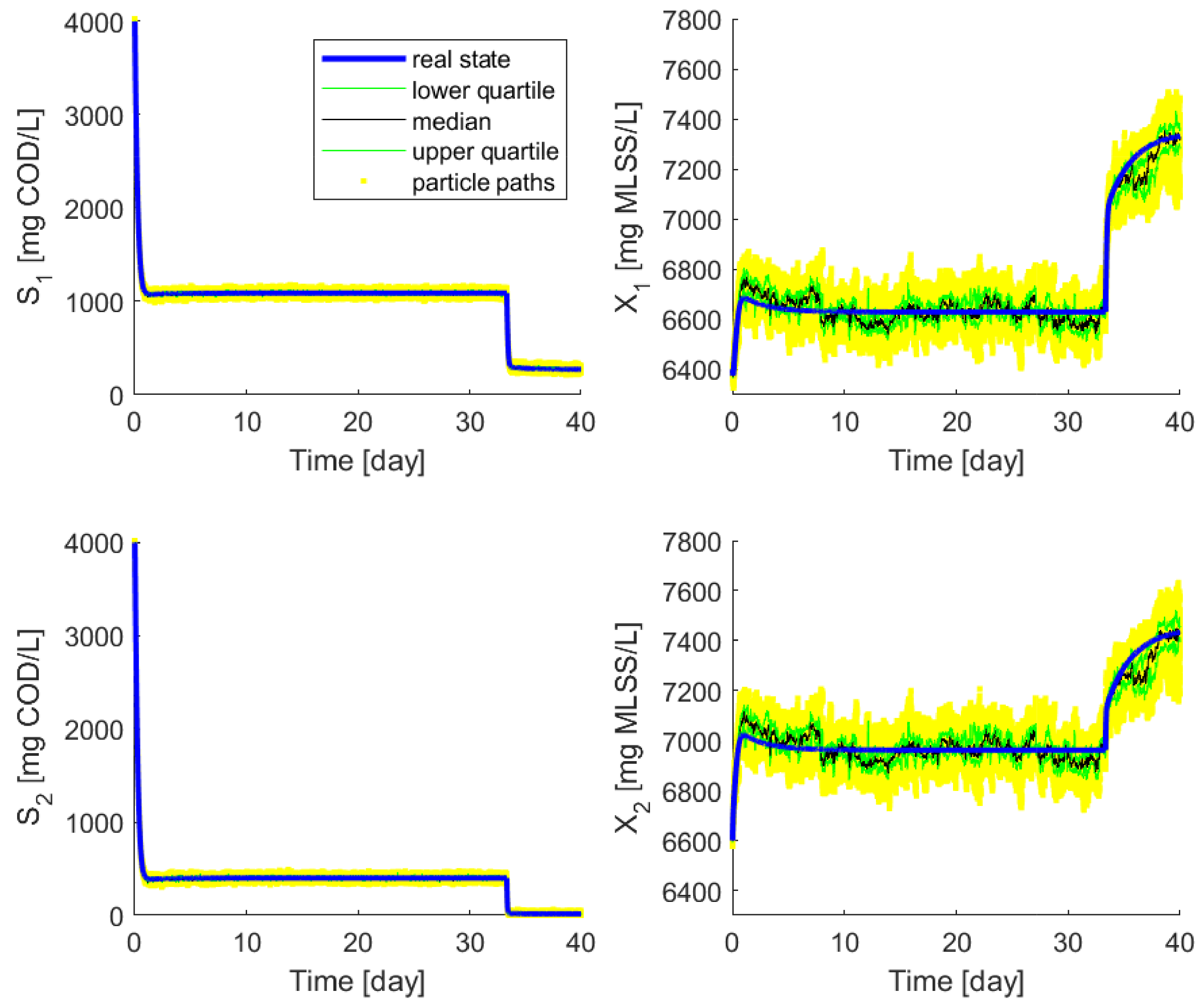
First of all, since the program had to be validated, it was tested to see if the estimated states followed the real states. State was measured first, as it is the most important of the four, being the one to be controlled. A total of 50 particles was used for the estimation.
The particle paths and the median of the particle states are in line with the real state represented by blue lines, as can be seen in
Figure 5. Although only the first 40 days were illustrated due to visibility, conclusions are the same throughout the entire time period.
Regarding the performed experiments, this MATLAB implementation of the PF works well and is suitable for further examinations.
3.3.1. Method of Sensor Placement
The next emerging issue is to determine which state variable is the most suitable to measure. Despite the fact that an explicit cost function is not available, the different configurations are comparable according to the estimation errors. Therefore, PF is used, the basic performance of which is satisfactory as introduced before. The placement of the sensor is determined by these measures before the PF is fine-tuned in
Section 3.3.2.
Online COD and suspended solids sensors are also used in wastewater treatment, such as in [
18], of different accuracies, namely:
for the former and about
for the latter. These values were used to define the standard deviations of the measurement noise in the simulation. Different measuring ranges in the two cases were also considered, so
was used for the COD and
for the suspended solids sensors.
Regarding the above-mentioned issues, the estimation performance was examined in all four cases by using 50 particles as well. For the evaluation, Equation (
8) was used to calculate the estimation error.
According to
Table 3, the cases when the concentration of microorganisms was measured produced much lower estimation errors because they are more sensitive to changes in the input variables, as seen in
Figure 4. Therefore, if the measured state is chosen from them, PF can provide a more accurate estimation. Another reason is that the measurement noises are relatively lower in these cases. The estimation performances are almost the same when comparing
and
as measured states. However, since the accuracy of
is the most crucial state in terms of the process control,
is measured in this wastewater treatment model.
Another interesting observation is that by considering the rows in
Table 3 separately, the same types of concentrations are almost identical. Moreover, any variation is always for the benefits the unmeasured state, e.g., when measuring
, the estimation of
is more accurate than that of
.
It is important to note that the results described above pertain to the actual process model with the current parameters. For example, the value of the measurement noise has a significant impact on them. However, besides the given parameters and state-space model, the optimal sensor location can be determined by the aforementioned method.
3.3.2. Sensitivity Analysis of the PF
As the previous example illustrated, some assumptions and parameters of the process significantly affect the effectiveness of state estimation. On the other hand, the parameters of the particle filter itself are also worth tuning. It was stated in
Section 2.4 that
exhibits an opposite effect on the estimation accuracy and simulation time. Therefore, this section aims to determine its optimal value for the present system.
Regarding the results of the
Section 4, we chose
as a measured state and executed the estimation using four different values of
. The results are depicted in
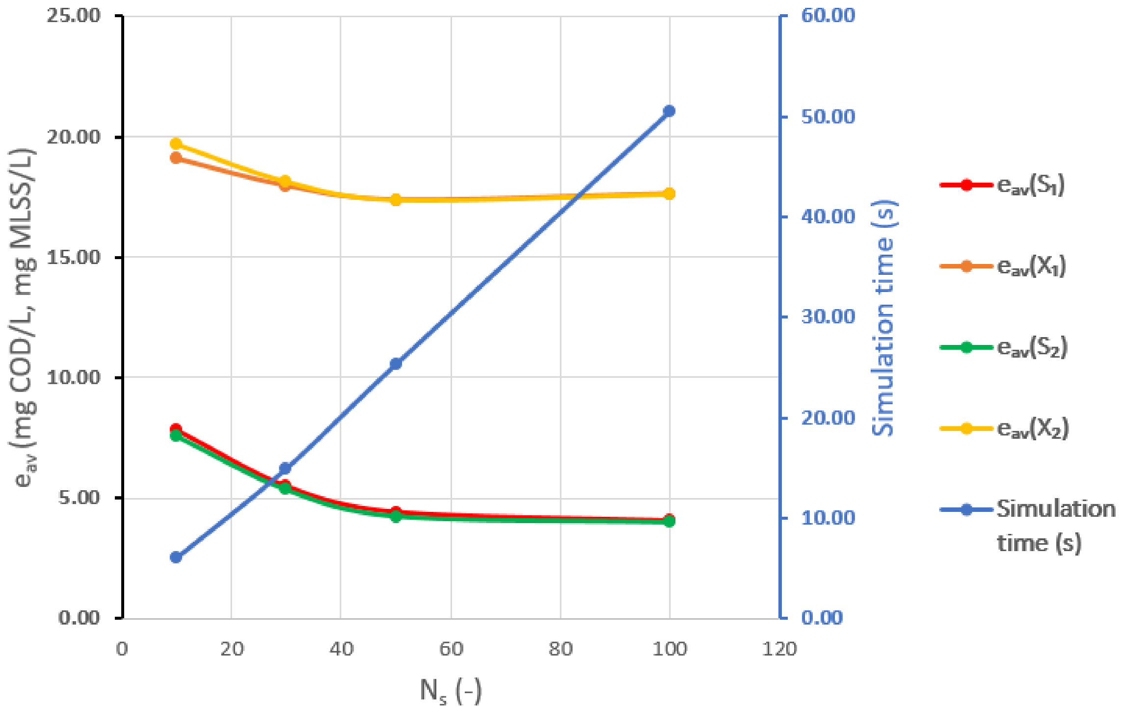
Figure 6.
During the evaluation, estimation errors were considered against the simulation time. The estimation errors decrease exponentially and become nearly constant beyond a determined value of
. On the contrary, the simulation time increases linearly as the number of particles rises. According to the curves of
Figure 6, the optimal
is about 30. Below this value, estimation errors increase rapidly, while above it, they remain nearly constant. For further investigations, this value will be used.
In the presented case study, the simulation time is not a crucial factor as the time constant of the system is a few days. However, for the state estimation of more complex systems with a shorter time constant, hundreds of particles may be needed and the simulation time can be a constraint, since it should always be lower than the sampling time of the system.
According to these principles, the parameter of the PF can be tuned in a similar manner, even for other processes.
3.3.3. PF and IPF Comparison
The simulation time and estimation errors are conflicting factors, as was seen in
Section 3.3.2. The question arises whether estimation accuracy could be increased without significant growth in the simulation time. A good opportunity in this regard is to test IPF in the present environment, which improves the level of efficiency by handling the phenomenon of sample impoverishment of general PF. IPF has not yet been applied in biochemical systems nor reactors. Its performance is tested in this section, besides setpoint changes.
The MATLAB program was coded according to the algorithm shown in [
10]. In order to be used, firstly, the two parameters (
,
) of the algorithm had to be tuned. This task was executed in a similar manner to the above-mentioned issues: by keeping in mind the average error, the optimal set of the parameters was determined. With this method,
and
were derived. Therefore, for the purpose of increasing the accuracy of the estimation, the particles only need to be better distributed in the same interval and it is not necessary to broaden it. From this result, it can be concluded that sample impoverishment is not a severe problem in this system. However, the level of efficiency could also be increased in this case by distributing the particles better.
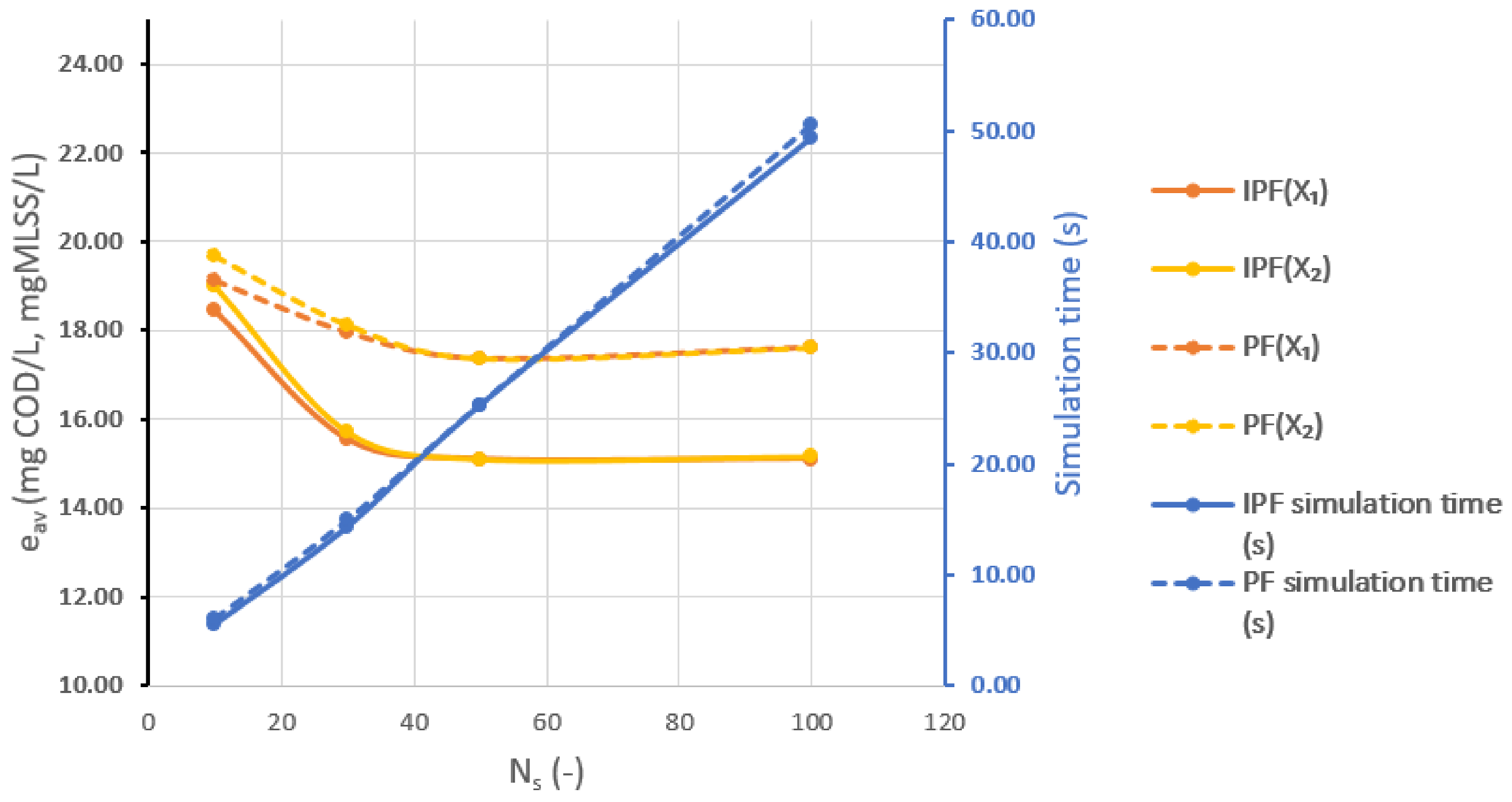
The tuned parameters were used to test the performance of the IPF compared to that of the PF.
The results are shown in
Table 4. It can be seen that the IPF performs better in all states but particularly in
and
. Although the IPF contains one more calculation step, the simulation times are almost identical because of the number of resamplings in the two cases. Investigating this issue, the average number of resamplings was 170 in the case of the PF and 158 in the case of the IPF (
). Therefore, if the IPF is used, resampling is needed less frequently.
Regarding the results of this section, it is recommended to use IPF instead of general PF to enhance the estimation accuracy.
As
Figure 7 and
Figure 8 present, the aforementioned conclusions also have pertinence in the case of different
values. Furthermore, it can be concluded that
is still the optimal value of the number of particles, even if IPF is applied.
To check if IPF’s performance is better than the PF’s even besides more setpoint changes, a longer part of the simulation was even used to compare the two algorithms in the case of the optimal . It contained three setpoint changes so that the dynamic behavior could be examined more profoundly. The conclusions were the same as above, namely the estimation error and number of resamplings were also lower in the case of IPF.
With this method, differences in the performances of the two algorithms can be investigated and the optimal value of the parameter determined.
3.4. Application of PF and IPF in Fault Diagnostics
With the carefully chosen and tuned MATLAB implementation of the particle filter, different fault detection problems can be solved. General PF and the IPF were also tested for this aim, and a comparison is presented in this section.
As state estimation with particle filters is based on the information gained from the process, it is essential to have fault-free measurement data. If the sensor is faulty, the estimation will be inaccurate, and it is not observable according to the estimation results. However, the particle filter is able to indicate the faults by following the method described in
Section 2.3.
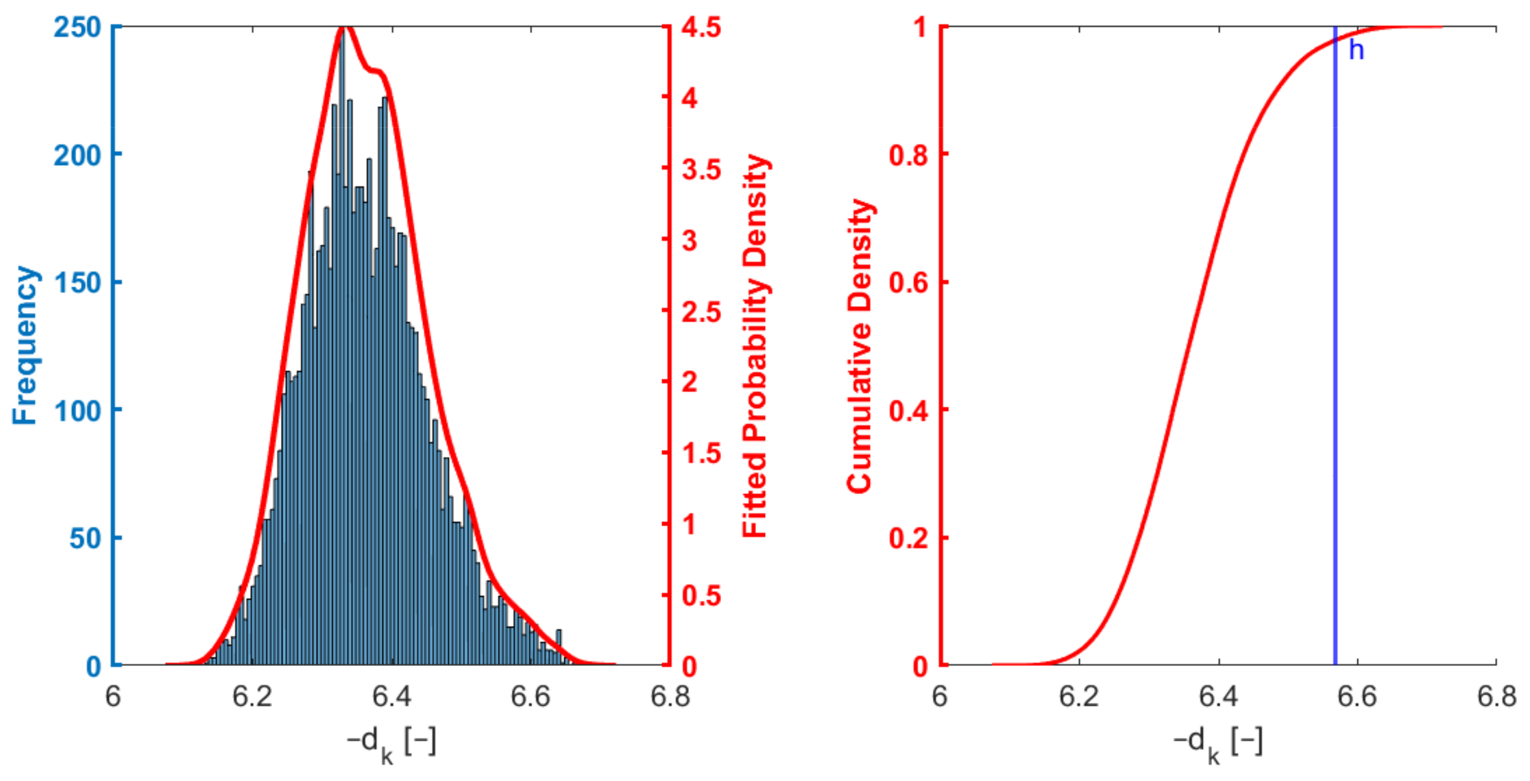
Fault occurrence is evaluated according to the value which is the negative sum of logarithms of the particle weights. If a faulty measurement occurs, the sum of the particle weights decreases, so increases. With a carefully chosen threshold, the fault can be detected.
First of all, the fault-free operation was tested, and the threshold belonging to its
confidence interval determined. Results are similar in the cases of general PF and IPF. The distribution of
values along with the threshold are shown in
Figure 9 in the case of the IPF.
3.4.1. Analysis of the Fault-to-Signal Ratio
A sensor fault can be modeled by an additive constant in the measurement function:
where
represents the fault. One of the main factors in fault detection is the fault-to-signal ratio. Therefore, the lowest value of
that can already be detected must be determined.
Four different values of
were examined: 5, 10, 15, and
of the value of measured state
at the first stationary state. The fault occurred on the 25th day and lasted until the 55th day, as is shown in
Figure 10. Furthermore, two setpoint changes were modeled around the 33rd and 66th days, one within the faulty time interval and the other after the fault had been rectified.
The results are illustrated in
Figure 11. It can be seen that
is quasi-constant during fault-free operations, so setpoint changes do not have an effect on it and the dynamic behavior of the process does not influence the efficiency of fault detection. Otherwise, the moment of fault occurrence is detected in all cases. However,
is once again quickly below the threshold in terms of the
and
faults. In the case of the
and
faults, it is above the threshold for almost the whole duration of the fault. As can be seen in
Figure 11, results are similar in the cases of general PF and IPF.
The aforementioned difference between the small and large fault amplitudes is explained by
Figure 12 and
Figure 13. These results show that in the case of minor faults, the estimated state is in line with the measured values after the fault occurs. However, in the case of the
fault, a residual error is recorded not only between the estimated and real states but even between the estimated and measured states. General PF and IPF behave similarly even in this case.
On the one hand, the reason for this phenomenon is that during the resampling step, the PF chooses new particles from the set of the prior particles. If the change is very significant, resampling cannot follow it. On the other hand, the particles try to converge with the real state as the state space model is deterministic.
For the aforementioned reasons, does not return to below the threshold while the fault lasts.
Once the fault has ceased,
returns to its initial value in all the cases in
Figure 11; moreover, the rectification of the fault is indicated by a spike.
It was noticed that in the case of minor faults, only the beginning and the end of the faulty time interval could be detected. However, considering the number of resamplings, information could be gained about the existence of the fault. As is shown in
Table 5, since the average number of resamplings per day is higher while the fault lasts, the duration of the fault can be unambiguously determined by following the tendency of
and the number of resamplings.
The effect of the setpoint changes is insignificant. In the case of the fault-free interval (setpoint change in
), the setpoint change is not perceptible in
Figure 11. The setpoint change in
F while the fault occurs is also negligible. For further investigations, the case of the
fault was chosen as it is the lowest that gives an alarm throughout the entire duration of the fault according to
. As general PF and IPF showed similar behavior, henceforth the IPF is used to present the results.
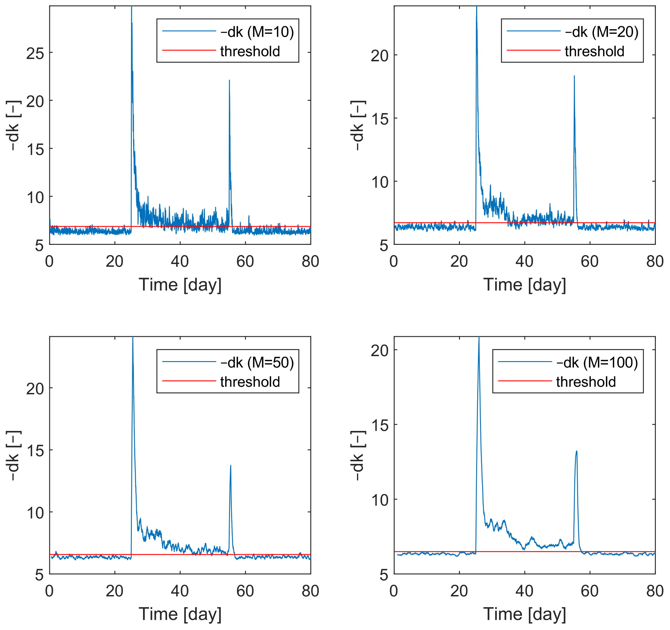
3.4.2. Tuning the Sliding Window
In the fault decision function (Equation (
12)), the
M sliding window parameter functions as a smoothing parameter. The effect of this parameter on the noisiness of the
signal is shown in
Figure 14. If
M is small, the fluctuations in
are large, while if
M is larger,
is more filtered.
To determine the optimal value of
M, impact faults were also considered. The results are shown in
Figure 15. It can be concluded that the larger
M is, the less acute the spikes are and the intensity of the fault signal decreases.
According to these aspects, if the aim is to rapidly detect impact faults and sudden changes, a smaller M is suggested. However, if the duration of the bias fault is wanted to be indicated, a larger M is preferred. In the present case, is optimal to detect both bias and impact faults.
Besides the conclusions already made, the aforementioned experiments also point out that the implementation of IPF instead of general PF does not require changes to be made to the fault detection method. It can also be applied as in the case of general PF and is able to detect both bias and impact faults with high efficiency.
The threshold values used above, calculated by the
confidence interval, are summarized in
Table 6. As the
M sliding window functions as a smoothing parameter, the larger
M is, the narrower the distribution of
that results. Therefore,
h decreases as
M increases.
In this section, a PF-based fault detection technique was introduced. Based on the given method, it is feasible to determine the h threshold of alarm generation as well as tune the value of the M sliding window according to how the system responds to bias and impact sensor faults. To detect the existence of bias faults more accurately, the number of resamplings should also be considered.
4. Conclusions
In complex process systems, a state observer is required to estimate the unmeasured states. As these systems are often nonlinear, a particle filter (PF) is suitable for the task.
The present research work aimed to investigate the applicability of a particle filter state observer in process systems for the purposes of state estimation and fault diagnostics tasks through a case study. The PF was validated for and implemented in the system as a state observer; moreover, unmeasured states were estimated based on the measured one.
One contribution of the paper is a method obtained to determine the optimal sensor placement. Based on the principles declared in this paper, the method is usable in all cases by applying the actual state-space model and parameters.
Another novelty is a technique for tuning the PF and a proposed sensitivity analysis. To increase the estimation accuracy, a new variant of the PF, the genetic algorithm-based IPF, was implemented and tested under setpoint changes. A case study was presented to compare the performances of the two algorithms.
The completed state estimation algorithm was also tested for fault detection problems. A PF-based fault detection technique was implemented and evaluated. The effect of the setpoint changes was examined and a tuning method presented for the sliding window by also taking into consideration the bias and impact faults.
As applications of PF in process engineering are scarce, this area formed the subject of our research. The aforementioned experiments were executed in a carbon-removal wastewater treatment process that consists of a two-element reactor cascade and a settling unit. After validating the wastewater treatment model, according to the dynamic analysis of the system, a proper set of setpoint changes was determined considering the physical constraints of the process. This scenario was used for further investigations.
The PF performed well in the benchmark system since the estimated states closely followed the real ones. According to the average values of the estimation errors (), the preferable measured state variable was chosen. Considering the simulation time and values, the optimal value of the parameter of the PF was determined. An IPF was implemented in the system and compared with the general PF. This improved method reduced the estimation errors and even the number of resamplings.
As for fault detection, bias and impact sensor faults were extensively analyzed. The thresholds of alarm generation were determined according to the output of the decision function and sensor faults with various amplitudes were examined to evaluate the efficiency of fault detection. A comparison was also made between general PF and IPF from fault detection aspects. The M parameter of the decision function was also tuned; moreover, it was declared that the number of resamplings is also worthwhile following. With the applied method, bias and impact faults were also detected highly efficiently.
In the future, several research directions are plausible, as the field of particle filtering is very diverse and understudied. For example, fault detection performance could be examined for actuator and process faults. It would also be interesting to investigate the applicability of the technique with regard to estimating inputs or parameters. In terms of chemical engineering, other operational units could be studied or PF could be tested with regard to process control.


