Real-Time Structure Generation Based on Data-Driven Using Machine Learning

Abstract

Topology optimization results are highly dependent on the given design constraints and boundary conditions. Moreover, small changes in initial design conditions can result in different topological configurations, which makes topology optimization time-consuming in a given design constraint domain and inefficient in structural design. To address this problem, a data-driven real-time topology optimization framework and method coupled with machine learning by using a principal component analysis algorithm combined with a feedforward neural network are developed in this paper. Meanwhile, through the offline training, the mapping relationship between initial design conditions and topology optimization results is obtained. From this mapping, we estimate the optimal topologies for novel loading configurations. Numerical examples display that the online prediction results are consistent with the results of the topology optimization method. Furthermore, the network parameters are calibrated, and accurate structure prediction is achieved based on the algorithm. In addition, this method ensures the accuracy of high-resolution structural prediction on the premise of small samples.

1. Introduction

With the increasing demand for structural functions, topology optimization has been introduced into various fields for structure design, such as aerospace, engineering applications, electronic devices, and biomedicine [1,2,3,4,5]. So far, topology optimization has been developed to be one of the most effective ways to acquire new structures satisfied various design requirements [6,7,8,9,10]. With the continuous improvement of the theoretical system of topology optimization, varieties of methods have been developed to achieve the optimization of structures. At present, the solid isotropic material with penalization (SIMP) method [11], level set method [12], and moving morphable components (MMC) method [13] are widely used and implemented in topology optimization. Additionally, the evolutionary structural optimization (ESO) method [14], genetic algorithm (GA) method [15], and phase field method [16] are also efficient methods for structure optimization. Multiple constraints such as stress constraints [17], multi-material constraints [18], and other constraints are habitually considered in topology optimization design. Moreover, for the structural design of additive manufacturing, the thickness constraint of the minimum printable thickness [19] and the printing angle are as well as considered during the molding process [20]. Therefore, topology optimization provides a reference for structural design, in which multiple constraints make the design results much closer to engineering practice. Compared to the traditional structure design, topology optimization under multiple constraints provides more ideas for structure design. However, the iterative process of optimizing calculation is extremely time-consuming unless the time of iteration is greatly reduced or replaced by another more efficient method.

The neural networks, providing convenience for people to reduce the time for calculation of topology optimization, have been proven to be powerful functions in data learning and generalization, which can be used in classification, clustering, and regression [21,22,23]. Many researchers have aimed to reduce the time of structural design by combining neural networks with the topology optimization method. Taking the topological optimization of the heat conduction problem as an example, Lin et al. [24] proposed a deep learning approach combining the traditional solid isotropic material with the penalization method to reduce the time consumption of the optimization process. Ulu et al. [25] established a mapping between the load and the optimization result based on the SIMP method combined with the neural network algorithm. The results indicate that the proposed method can successfully predict the optimal topologies in novel loading configurations and also can be used as effective initial conditions for conventional topology optimization routines, resulting in substantial performance gains. Lei et al. [26] established a mapping between the load and optimization results on the basis of MMC combined with the supported vector regression (SVR)/K-nearest neighbors (KNN) algorithm. The training data and dimension of parameter space are substantially reduced. Yu et al. [27] solved the problem of low sample resolution by using generative adversarial networks (GAN) in view of the establishment of a predictive network with convolutional neural networks (CNN). The proposed method can determine a near-optimal structure in terms of pixel values and compliance with negligible computational cost. Cang et al. [28] proposed a theory-driven mechanism for a neural network model that performs generative topology design in one shot given a problem setting, circumventing the conventional iterative process. Thus, it can be seen, the combination of topology optimization and neural network learning is an effective way to reduce the cost of computation. However, the aforementioned methods still have some problems. For example, some methods only accelerate a portion of the optimization process, some methods have a low dataset and small sample size that is not enough to explain various problems, and some methods need a huge sample size and expensive calculation cost. Based on these observations, a data-driven real-time topology optimization framework and method coupled with machine learning are developed. The relationship between initial design conditions and topology optimization is obtained. The results ensure the accuracy of high-resolution structural prediction under the premise of small samples.

The remaining sections are organized as follows. Section 2 presents the structural optimization theory and numerical examples. Section 3 describes the construction of neural networks and the theory of dimension reduction algorithms in detail. The effects of various network parameters are also discussed. Finally, the advantages and disadvantages of this method are systematically described, and the corresponding solutions are proposed.

2. Structural Optimization Theory and Data Sample

The purpose of topology optimization is to provide the best material distribution in the designated design area according to the given load and boundary conditions. In other words, a certain mechanical performance index of the optimized configuration can reach the maximum value. Messerschmitt–Blkow–Blohm (MBB) beam problem is used as an example of real-time topology optimization implementation in this study. In the MBB model, the length and width of the beam are represented by N_x and N_y, respectively. The design domain is discretized into N_x × N_y rectangular grids for finite element calculations, and the density $\rho$ of each element controls the presence or absence of the material. F(x, y) describes the load at the x, y points in the Cartesian coordinate system as seen in Figure 1. To reduce the amount of calculation, the beam is processed symmetrically and the DOF (degree of freedom) of x in the middle part is constrained.

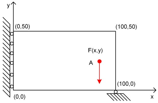
Figure 1. Design domain and load distribution of the MBB beam.

The goal of topological optimization is to seek the topological configuration of the MBB beam with maximum stiffness at a specific volume fraction. The objective function, C, represents the work performed by various configurations under load. The optimal solution is obtained by seeking the minimum value of the objective function. In the present research, the goal of topology optimization is maximum stiffness, and the objective function is equivalent to minimum compliance. The constraints can be described as volume constraints, equilibrium equations, and density constraints, so the problem description can be expressed as Equation (1):

$${\min }_x:c(x)=U^{T}GU={\displaystyle \sum _{j=1}^N{E}_j(x_j)u_j^T}{g}_j{u}_j$$

$$st:\frac{V(x)}{V_0}=f$$

(1)

$$:GU=F$$

$$:0<x_{\min }\le x_j\le 1$$

where U and F are the displacements and global force, respectively. G is the global stiffness matrix. g_j and u_j are the stiffness matrix and displacement vector of the element. x_j is the design variable. V and V₀ are the design material volume and design area volume.

The density interpolation function is chosen to give the modulus of the element as Equation (2):

$$E_j=E_{\min }+x_j^p(E_0-E_{\min })\hspace{1em}{x}_j\in [0,1]$$

(2)

where E₀ and E_min are the material modulus and minimum modulus, respectively. p is the penalty coefficient of the modulus, which is set to 3 here.

A batch of random loads is used as input data for the topology optimization program, and a series of optimization results (1500) is obtained as a database. The input of the topology optimization program TOP88 is set to (100, 50, 0.25, 3, 1.5, 1, F(x,y)), which corresponds to (nelx, nely, volfrac, penalization coefficient, filter radius, filter function, load coordinates). The topology optimization program in this paper is adapted from the program of the group of Andreassen et al. [29], and part of the optimization results are exhibited in Figure 2. The red arrow in Figure 2 represents load, and the value of C indicates compliance.

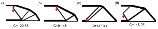
Figure 2. Part of structural optimization results (the red arrow indicates load, and the value of C indicates compliance) with different values of C. (a) C = 120.58, (b) C = 91.45, (c) C = 137.93, (d) C = 148.05.

3. Deep Learning and Training

The MATLAB toolbox is used to build a neural network for predicting topology-optimized structural designs. The network is divided into two stages: the offline training stage and the online prediction stage. Before the offline training, the sample should be collected by the topology optimization program as the training set and contrast set. Then, the network is built by using a principal component analysis (PCA) algorithm combined with a feedforward neural network. Firstly, the training samples are reduced to the feature image by the PCA algorithm. Secondly, the load–weight relationship is established by the feedforward neural network. Finally, the relationship between the load and the optimization result is obtained. Based on the above stages, new load information is selected and input into the neural network to return a new weight W by online prediction, and real-time topology optimization is realized.

3.1. Data Reduction

The PCA algorithm is a dimensionality reduction method for preprocessing high-dimensional feature data, which improves the data processing speed by removing noise [30]. The optimization results need to be reduced to gain a certain number of feature images via the PCA algorithm before training. The PCA algorithm flow is shown in Figure 3. If the design domain size is N_x × N_y matrix, the single optimization result is represented by a matrix of rows. Then, the result of optimization O is a K × L matrix, and the centralized image of the result can be expressed as $Y_j=O_j-\overline{O}$, where $\overline{O}$ is the mean value of the optimization result. In order to reduce the dimension of data, the covariance matrix $C=Y{Y}^T$ is constructed. The C is a K-order square matrix with K eigenvectors, and the eigenvectors with smaller eigenvalues are unimportant features. According to the size of eigenvalues, the first M-order eigenvectors are selected as the new covariance matrices J, which is the result of PCA dimensionality reduction (M << K).

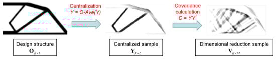
Figure 3. The process and principle of data reduction algorithm.

The eigen-images shown in Figure 3 are calculated as $V=Y^{T}J$, where V equals to K × M. It indicates that the optimization results can be linearly combined by these eigen-images. An equation of a linear mapping relationship between optimization results and eigen-images $O_{K\times L}$ established as Equation (3):

$$O=W{V}^T\hspace{1em}{W}_i={[W_1,W_2,\dots ,W_k]}^T$$

(3)

where W is the mapping weight.

The original K optimization results are integrated into M eigen-images by the PCA method for data dimensionality reduction. The weight W corresponding to the new design condition is the key to realizing real-time topology optimization. Subsequently, establishing the mapping relationship between load F and weight W is necessary.

3.2. Feedforward Neural Network

It is well known that a feedforward neural network is the most widely used neural network, which can realize the functions of classification, regression, and clustering. The regression function can be used to express the mapping relationship between load and eigen-image. Generally, the network can be divided into the input layer, the hidden layer, and the output layer. A four-layer feedforward neural network is shown in Figure 4. The information obtained from the input layer is transmitted to the hidden layer for training, and then the trained information goes into the output layer and returns the output value. This process of offline training is to train a feedforward neural network and establish the nonlinear mapping relationship between load F_i and weight W_i. The load information F_i is an input and the weight W is set as a label. Trainlm is selected as the training function, the learning function is learngdm, and the mean square error is used to calculate the error of samples. The trained network can realize online prediction, and real-time topology optimization can be achieved by combining the PCA algorithm.

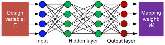
Figure 4. The online prediction realization using the neural network.

3.3. The Implementation of Real-Time Topology Optimization Algorithm

The real-time topology optimization is generally divided into four stages, as shown in Figure 5. The first stage is sample collection, in which the training set and contrast set are obtained through the topology optimization program. The second stage is the data dimension reduction stage. In this stage, the training set is transformed into a featured image by the PCA algorithm, and the linear mapping relationship is established to obtain the weight W. The third stage is the offline training stage, in which the load information corresponding to the training set is input and labeled as weight W to train the neural network. The fourth stage is the final online prediction stage. New load information is selected and input into the neural network to return the new weight W, and new optimization results are obtained by combining the eigen-images. The online prediction phase is completed instantaneously, which represents the realization of real-time topology optimization.

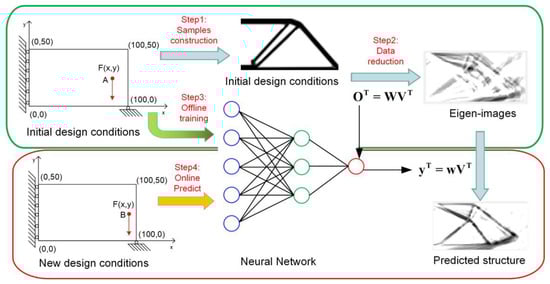
Figure 5. Process for real-time topology optimization implementation.

3.4. Discussion on Network Parameters

The training effect involves many parameters, such as the number of samples D, the size of design domain L, the number of feature images M, the number of layers H of the neural network, and the amount of neurons N. In order to determine the optimal value of the parameters, the control variable method is used to analyze the influence of the parameters. The TRAINLM function is selected as the training function, the LEARNGDM function as the adaptation learning function and the TANSIG function is selected as the regularization function. Meanwhile, the function of subsequent network training settings remains the same. The prediction accuracy is expressed by the mean square error (MSE) as Equation (4):

$$MSE=\frac{1}{D}{\displaystyle \sum _{d=1}^D(y_d}-{\overline{y}}_d{)}^2$$

(4)

where D is the number of samples, and the $y_d$ is the density value of the predicted structure.

It is very important to determine the influence of eigen-images M on network training. Considering the computational efficiency, 500 samples are used to train the network. The layer of networks is set to 2, the neurons are set to 100, and the eigen-images M is taken from 10 to 200. One of the optimization results is selected to compare with the predicted results as shown in Figure 6.

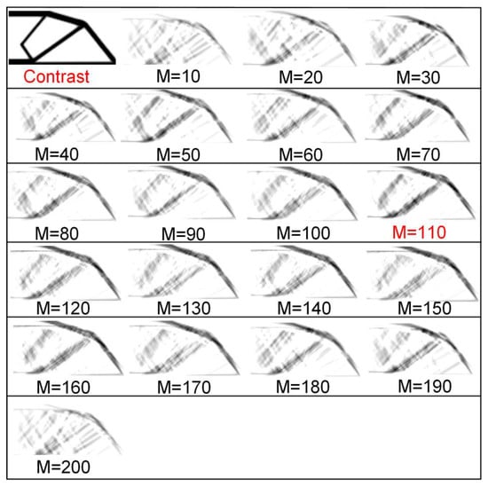
Figure 6. The prediction result of training 1 with different M.

The number of neurons N is one of the parameters of neural network. It is necessary to analyze the influence of the number of neurons on network training. Considering the computational efficiency, 200 samples are used to train the network. The layers of network are set to 2, the eigen-images are set to 20, and the numbers of neurons are taken from 10 to 150 to produce 15 sets of samples for training. The prediction images are shown in Figure 7.

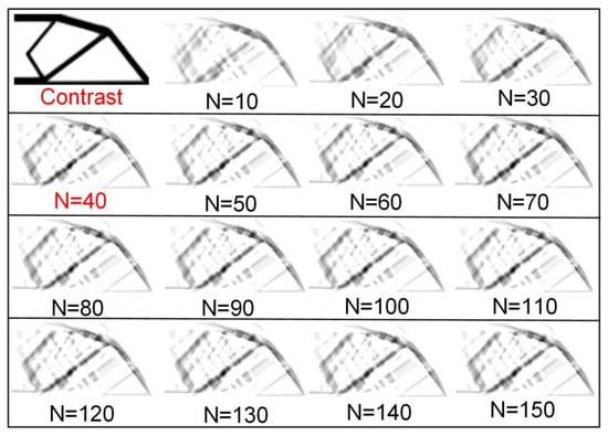
Figure 7. The prediction result of training 2 with different N.

Figure 8 displays the error analysis in view of the M and the N. When M is in the range of 15–25% of the sample size, the error is stable at the range of 2.65–2.7%, and the minimum error is 2.663% when M is 22% of the sample size D. The same trend is also reflected in the prediction image. When M is 110, the best prediction effect is obtained. When M is greater than 130, the image begins to appear over-fitting. This is because the excessive value of M leads to unnecessary features and too small a value of M leads to the phenomenon of under-fitting as well. The error analysis indicates that when N is in the range of 15–30% of the sample size, the error is stable at 3.6–3.8%, and the minimum error is 3.658% when M is 20% of the sample size. This is also reflected in the prediction image. When N is 40, the best prediction effect is obtained. When N is greater than 100, the image begins to appear over-fitting. This is also because the excessive value of N leads to unnecessary features, and too small a value of N leads to the phenomenon of under-fitting. It is obvious that the training effect is optimal when N ≈ M. According to the results obtained by analyzing the errors of the control variables, when the values of the M and the N are both at 20% of the training samples, the minimum prediction error is obtained. It is not difficult to understand from the principle of neural networks, each neuron corresponds to an intrinsic image. In this way, when the weights are mapped as labels, a better training effect can be achieved.

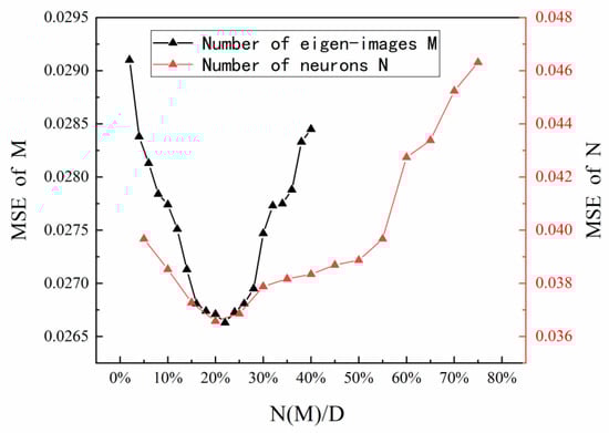
Figure 8. The influence of number of feature images and number of neurons on prediction accuracy.

As for depth H of the network, the most basic structure is the two-layer structure with one hidden layer and one output layer. When the number of hidden layers is over two, it is called a deep neural network. In order to determine the influence of H, 200 samples are used to train the network. The number of neurons N is set to 20, the number of eigen-images M is set to 20, and the number of hidden layers is taken from 2 to 8 to produce 7 sets of samples for training. The prediction images and the errors are shown in Figure 9 and Figure 10, separately. The error analysis indicates that when the value of H goes into 2–5, the error is less than 3.8%. When H is greater than 5, the image begins to appear over-fitting. The error of the three-layer network and four-layer network is 3.742% and 3.764%, respectively. Considering the computational cost, the number of hidden layers is set to 2.

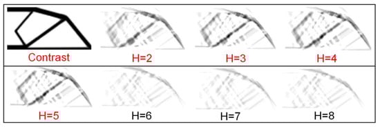
Figure 9. The prediction result of training 3 with different H.

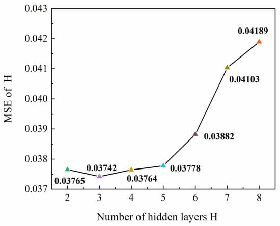
Figure 10. The influence of the number of network layer on prediction accuracy.

In order to analyze the influence of the number of samples D, the layer of the network is set to 2, the eigen-images M are set to 20 and the number of neurons N is set to 20. The number of samples is taken from 100 to 1400. The prediction images are shown in Figure 11. It indicates that when the number of samples exceeds 500, the detail loss and prediction errors begin to appear on the prediction images, which is not consistent with common sense. This is because the values of N and M do not change with the number of samples, which leads to the inadequacy of network fitting ability. When the number of samples ranges from 100 to 400, the proportion of M is in 5–20%, which further validates the previous conclusion of the M value.

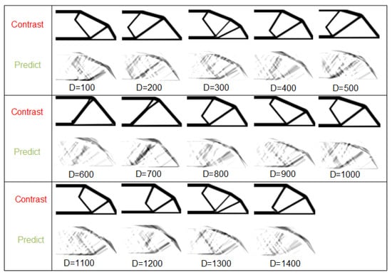
Figure 11. Initial prediction result of training 4 with different D.

3.5. Realization of Real-Time Topology Optimization

An efficient real-time topology optimization network is established through parameter impact analysis, which gives an accurate calibration of the network parameters. Based on the research, the prediction effect of real-time topology optimization is first determined by the sample size, and a sufficient number of samples can compensate for the problem of insufficient network fitting ability to some extent. When the number of neurons is about 20% of the sample size, the network fitting ability is the strongest. Under the premise of comprehensively considering the calculation and calculation consumption, a proper increase in the number of layers of the neural network can obtain a better prediction effect.

After the parameter calibration, the value or value range of the network parameters are determined. The number of neurons in the input layer is equal to the first dimension K of the weight w, and the number of neurons in each hidden layer is coincident with the input layer. The number of neurons in the output layer is concurrent with the dimension of the label (load), which is set constant to 2. The number of hidden layers is set to 2. As shown in Table 1, the value of eigen-images M and the number of neurons N are adjusted according to the value of sample size D. The prediction images are shown in Figure 12, and the errors are shown in Figure 13, respectively. As can be seen from the two figures, in the beginning, the prediction effect is very poor due to the lack of sample sizes. As the number of samples increases, the accuracy of image prediction increases synchronously. When the D reaches 500, the results are predicted as acceptably accurate. When D is 500,600,700, the network training time is 121.43 S, 178.54 S, and 252.76 S, respectively. The new load conditions are printed into the network, and the online prediction time is only 10-2 S, which is realized in real-time topology optimization. The prediction accuracy can be improved by segmenting and filtering the results of the preliminary prediction.

Table 1. Network parameter setting.

Design Domain Size L	Sample Size D	Eigen-Images Size M	Neurons Size N	Number of Hidden Layers H
100 × 50	100	20	20	2
100 × 50	200	40	40	2
100 × 50	300	60	60	2
100 × 50	400	80	80	2
100 × 50	500	100	100	2
100 × 50	600	120	120	2
100 × 50	700	140	140	2

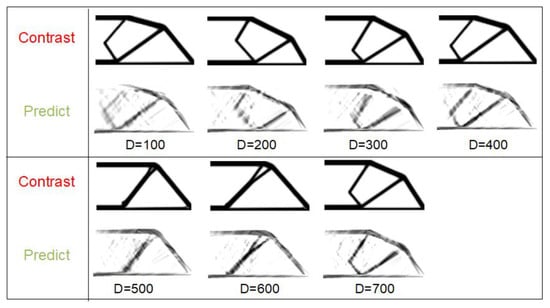
Figure 12. The prediction result after adjusting parameters of training 4 with different D.

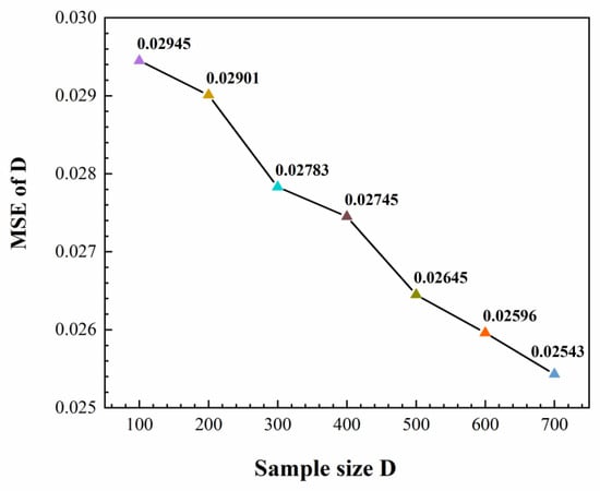
Figure 13. The influence of the sample size D on prediction accuracy.

4. Results and Discussion

A topology optimization model based on artificial neural network learning is proposed. Through the PCA algorithm, the training data are screened in advance to eliminate interference or redundant data and the data dimension is reduced. Then, through the comparative analysis of different training network parameters, the best training framework is found, so that it can obtain more accurate prediction results with less sample data.

Compared with the work of Ulu et al. [25], our algorithm particularly studies the influence of dimensionality reduction parameters and neural network parameters on the prediction results. Selecting appropriate parameters can significantly reduce the offline training data samples required for network training, and the prediction structure is more accurate.

Compared with the convolutional decoding and coding network adopted by Yu et al. [27], our network adopts the architecture of data dimensionality reduction and a full connection network. Before network training, we preprocess the samples by means of data dimensionality reduction to remove redundant information. Therefore, compared with Yu et al. [27] using 10,000 training samples to achieve accurate prediction of the structure, our algorithm can achieve the same effect with only 700 samples, that is, our algorithm has less sample dependency and stronger learning ability.

5. Conclusions

This study proposes a data-driven real-time topology optimization method that combines data dimensionality reduction with machine learning to achieve a design structure at the instant of a given design condition. The impact of the network parameters on the prediction accuracy is discussed and then the optimal parameter configuration scheme is obtained. It indicates the network prediction effect is the best when the number of hidden layers H is two and the number of neurons N is at 20% of the number of samples. In addition, when the number of samples K is greater than 500 as a threshold, the network error converges, and it decreases with the increasing number of samples.

The predicted image obtained by this method has higher resolution and more computational efficiency, and the demand sample is less. However, this method has certain limitations. Although the generation of the load is random, the boundary conditions in the example are fixed. This limitation can be solved by a combination of boundary conditions and loads. This study demonstrates the advantages of combining machine learning with topology optimization and broad development prospects, providing more efficient and accurate optimization methods and tools for structural design.

References

- Hanush, S.S.; Manjaiah, M. Topology optimization of aerospace part to enhance the performance by additive manufacturing process. Mater. Today Proc. 2022, 62, 7373–7378. [Google Scholar] [CrossRef]
- Zhou, H.M.; Zhang, B.; Shao, X.Y.; Tian, Y.P.; Guo, W.; Gu, Q.; Wang, T. Adaptive compensation method for real-time hybrid simulation of train-bridge coupling system. Struct. Eng. Mech. 2022, 83, 93–108. [Google Scholar] [CrossRef]
- Han, Z.; Wang, Z.; Wei, K. Shape morphing structures inspired by multi-material topology optimized bi-functional metamaterials. Compos. Struct. 2022, 300, 116135. [Google Scholar] [CrossRef]
- Zhao, Z.; Zhang, X.S. Topology optimization of hard-magnetic soft materials. J. Mech. Phys. Solids 2022, 158, 104628. [Google Scholar] [CrossRef]
- López, J.; Valizadeh, N.; Rabczuk, T. An isogeometric phase–field based shape and topology optimization for flexoelectric structures. Comput. Methods Appl. Mech. Eng. 2021, 391, 114564. [Google Scholar] [CrossRef]
- Zeng, T.; Wang, H.; Yang, M.; Alexandersen, J. Topology optimization of heat sinks for instantaneous chip cooling using a transient pseudo-3D thermofluid model. Int. J. Heat Mass Transf. 2020, 154, 119681. [Google Scholar] [CrossRef]
- Sahimi, M.; Tahmasebi, P. Reconstruction, optimization, and design of heterogeneous materials and media: Basic principles, computational algorithms, and applications. Phys. Rep. 2021, 939, 1–82. [Google Scholar] [CrossRef]
- da Silveira, T.; Baumgardt, G.; Rocha, L.; dos Santos, E.; Isoldi, L. Numerical simulation and constructal design applied to biaxial elastic buckling of plates of composite material used in naval structures. Compos. Struct. 2022, 290, 115503. [Google Scholar] [CrossRef]
- Uddin, M.; Haq, S. RBFs approximation method for time fractional partial differential equations. Commun. Nonlinear Sci. Numer. Simul. 2011, 16, 4208–4214. [Google Scholar] [CrossRef]
- Jensen, P.D.L.; Sigmund, O.; Groen, J.P. De-homogenization of optimal 2D topologies for multiple loading cases. Comput. Methods Appl. Mech. Eng. 2022, 399, 115426. [Google Scholar] [CrossRef]
- Yarlagadda, T.; Zhang, Z.; Jiang, L.; Bhargava, P.; Usmani, A. Solid isotropic material with thickness penalization—A 2.5D method for structural topology optimization. Comput. Struct. 2022, 270, 106857. [Google Scholar] [CrossRef]
- Nguyen, S.H.; Nguyen, T.N.; Nguyen-Thoi, T. A finite element level-set method for stress-based topology optimization of plate structures. Comput. Math. Appl. 2022, 115, 26–40. [Google Scholar] [CrossRef]
- Wang, L.; Shi, D.; Zhang, B.; Li, G.; Liu, P. Real-time topology optimization based on deep learning for moving morphable components. Autom. Constr. 2022, 142, 104492. [Google Scholar] [CrossRef]
- Zhang, J.; Chen, Y.; Zhai, J.; Hou, Z.; Han, Q. Topological optimization design on constrained layer damping treatment for vibration suppression of aircraft panel via improved Evolutionary Structural Optimization. Aerosp. Sci. Technol. 2021, 112, 106619. [Google Scholar] [CrossRef]
- Garus, S.; Sochacki, W. Structure optimization of quasi one-dimensional acoustic filters with the use of a genetic algorithm. Wave Motion 2020, 98, 102645. [Google Scholar] [CrossRef]
- Li, P.; Wu, Y.; Yvonnet, J. A SIMP-phase field topology optimization framework to maximize quasi-brittle fracture resistance of 2D and 3D composites. Theor. Appl. Fract. Mech. 2021, 114, 102919. [Google Scholar] [CrossRef]
- Yang, D.; Liu, H.; Zhang, W.; Li, S. Stress-constrained topology optimization based on maximum stress measures. Comput. Struct. 2018, 198, 23–39. [Google Scholar] [CrossRef]
- Zhang, W.; Song, J.; Zhou, J.; Du, Z.; Zhu, Y.; Sun, Z.; Guo, X. Topology optimization with multiple materials via moving morphable component (MMC) method. Int. J. Numer. Methods Eng. 2017, 113, 1653–1675. [Google Scholar] [CrossRef]
- Zhang, W.; Zhong, W.; Guo, X. An explicit length scale control approach in SIMP-based topology optimization. Comput. Methods Appl. Mech. Eng. 2014, 282, 71–86. [Google Scholar] [CrossRef]
- Guo, X.; Zhou, J.; Zhang, W.; Du, Z.; Liu, C.; Liu, Y. Self-supporting structure design in additive manufacturing through explicit topology optimization. Comput. Methods Appl. Mech. Eng. 2017, 323, 27–63. [Google Scholar] [CrossRef]
- Aswathi, R.R.; Jency, J.; Ramakrishnan, B.; Thanammal, K. Classification Based Neural Network Perceptron Modelling with Continuous and Sequential data. Microprocess. Microsyst. 2022, 104601, in press. [Google Scholar] [CrossRef]
- Djenouri, Y.; Belhadi, A.; Lin, J.C.-W. Recurrent neural network with density-based clustering for group pattern detection in energy systems. Sustain. Energy Technol. Assess. 2022, 52, 102308. [Google Scholar] [CrossRef]
- Surendranatha, G.; Naidu, B.V.V.; Gangaraju, M.; Sarapure, S.; Hemanth, K. Development of predictive models for wire electrical discharge machining of aluminium metal matrix composites by using regression analysis and neural network. Mater. Today Proc. 2022, 68, 1581–1587. [Google Scholar] [CrossRef]
- Lin, Q.; Hong, J.; Liu, Z.; Li, B.; Wang, J. Investigation into the topology optimization for conductive heat transfer based on deep learning approach. Int. Commun. Heat Mass Transf. 2018, 97, 103–109. [Google Scholar] [CrossRef]
- Ulu, E.; Zhang, R.; Kara, L.B. A data-driven investigation and estimation of optimal topologies under variable loading configurations. Comput. Methods Biomech. Biomed. Eng. Imaging Vis. 2016, 4, 61–72. [Google Scholar] [CrossRef]
- Lei, X.; Liu, C.; Du, Z.; Zhang, W.; Guo, X. Machine Learning-Driven Real-Time Topology Optimization Under Moving Morphable Component-Based Framework. J. Appl. Mech. 2019, 86, 11004. [Google Scholar] [CrossRef]
- Yu, Y.; Hur, T.; Jung, J.; Jang, I.G. Deep learning for determining a near-optimal topological design without any iteration. Struct. Multidiscip. Optim. 2019, 59, 787–799. [Google Scholar] [CrossRef]
- Cang, R.; Yao, H.; Ren, Y. One-shot generation of near-optimal topology through theory-driven machine learning. Comput. Des. 2019, 109, 12–21. [Google Scholar] [CrossRef]
- Andreassen, E.; Clausen, A.; Schevenels, M.; Lazarov, B.S.; Sigmund, O. Efficient topology optimization in MATLAB using 88 lines of code. Struct. Multidiscip. Optim. 2011, 43, 1–16. [Google Scholar] [CrossRef]
- Jiang, J.-H.; Wang, J.-H.; Chu, X.; Yu, R.-Q. Neural network learning to non-linear principal component analysis. Anal. Chim. Acta 1996, 336, 209–222. [Google Scholar] [CrossRef]
Disclaimer/Publisher’s Note: The statements, opinions and data contained in all publications are solely those of the individual author(s) and contributor(s) and not of MDPI and/or the editor(s). MDPI and/or the editor(s) disclaim responsibility for any injury to people or property resulting from any ideas, methods, instructions or products referred to in the content. |
© 2023 by the authors. Licensee MDPI, Basel, Switzerland. This article is an open access article distributed under the terms and conditions of the Creative Commons Attribution (CC BY) license (https://creativecommons.org/licenses/by/4.0/).