The Influence of Sample Size on Long-Term Performance of a 6σ Process

Abstract

There are many criticisms for the association between the Six Sigma concept and the two statistical metrics associated to 6σ processes: 1.5σ shift for maximum deviation and 3.4 PPM non-conformities for the long-term performance. As a result, the paper aims to carry out an analysis of this problem, and the first result obtained is that a stable process can reach a maximum drift, but its value depends on the volume of the sample. It is also highlighted that, using only the criterion “values outside the control limits” for monitoring stability through the Xbar chart, a minimum value can be calculated for the long-term performance of a process depending on the sample size. The main conclusion resulting from the calculations is that, in the case of a 6σ process, the long-term performance is much better than the established value of 3400 PPB: For small volume samples of two pieces it is below 700 PPB, for three pieces it is below 200 PPB, and for samples with a volume greater than or equal to four pieces the performance already reaches values below 100 PPB! So, the long-term performance of 6σ processes is certainly even better than the known value of 3.4 PPM.

1. Introduction

The Six Sigma method is an extremely well-known concept in quality theory, interpreted over time as a metric, methodology, or a management system.

The notation 6σ is used when the approach is mathematical otherwise “Six Sigma” formula is used. In this way the difference is made between the capability index (mathematical concept) and the capability of the process (characteristic of the process).

As a methodology or a management system, there are two ways of implementation regarding the processes: DMAIC (Define, Measure, Analyze, Improve, Control) for quality improvement, and DMADV (Define, Measure, Analyze, Design, Verify) for the design of the process [1,2].

The lean manufacturing concept is associated with the Lean Six Sigma method [3,4,5] and involves the use of various quality-specific tools. There is a rich body of literature on the Lean Six Sigma concept and its implementation [6,7,8], including following well defined logic schemes [3,9,10].

As a metric system, there are many possibilities for exploration, especially because of numerous criticisms [11,12,13], the most concrete being those that refer to the two statistical concepts associated with the method to characterize the long-term process: The 1.5σ deviation shift and the proportion of non-conformities 3.4 PPM.

However, in order to understand how the Six Sigma method was created and its association with the two statistical quantities, 1.5σ Shift and 3.4 PPM (parts per million) or 3400 PPB (parts per billion), it is important to present how the Six Sigma method appeared and evolved.

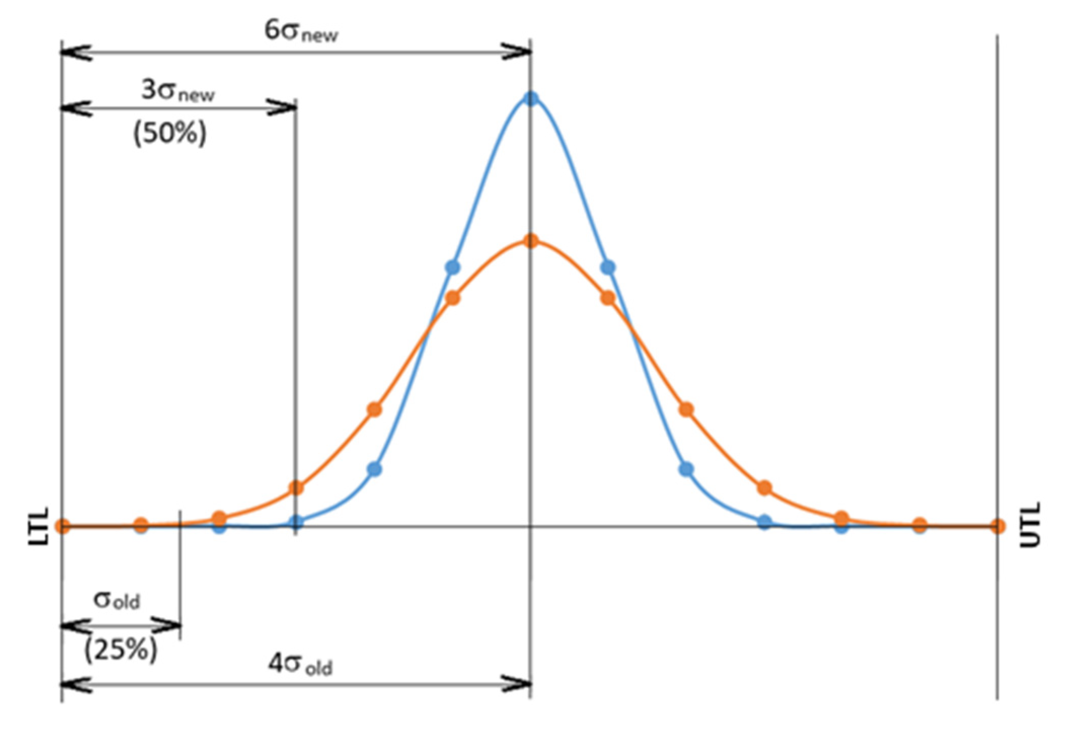
In order to overcome the problems due to the inadequate quality of the products, in 1986 the Motorola company initiated a quality improvement program under the guidance of the engineer Bill Smith [14,15,16], who proposed that the products had to be made more precisely in relation to the specification and established the following objective: For the essential characteristics to reach a superior precision, for which the limits of the tolerance interval (lower tolerance limit, LTL; upper tolerance limit, UTL) should be at a distance of ±6σ_new compared with the mean of the centered process. The old precision (corresponding to a minimum capability C_pk = 1.33) assumed that the tolerance limits were only at a distance of at least ±4σ_old from the process average.

In accordance with the 3 sigma rule from statistical quality control, it is considered that no defects appear beyond the interval ±3σ compared with the average. The ratio between the domain situated beyond the tolerance interval where no defects appear (beyond ±3σ compared with average) and the size of the tolerance interval will increase from the value of 25% (result from the ratio σ_old/4σ_old), to the value of 50% (result from the ratio 3σ_new/6σ_new). So it can be said that, in this way, the relative size of the safety zone is doubled.

Process precision is highlighted in Figure 1, where the following essential aspects can be observed: The improvement in quality is not made by widening the tolerance interval, but by improving the precision of the process, which is why two distributions of the values are represented in the image—the initial one (precision 4σ_old), and the new one (precision 6σ_new).

This is not as relevantly highlighted, even by the person who implement Bill Smith’s idea and who is associated with the new concept—Michael Harry [15]—nor by other authors who present the origin of the concept [16,17].

The approach regarding increasing precision as an efficient way to improve quality is also supported by Montgomery [18], who says: “Quality is inversely proportional to variability”. Likewise, Bass [19] states: “Variability: The source of defects”.

However, this is the ideal case, which can be valid at an initial moment (immediately after adjusting the process), the so-called short-term performance, for which the proportion of non-conformities is 2·F(6σ) = 2·0.0001 = 0.0002 PPM (parts per million), where F(x) is the integral Laplace function. In the long term, however, it must be accepted that the process will not remain perfectly centered, and it will have a certain drift in relation to the initial position.

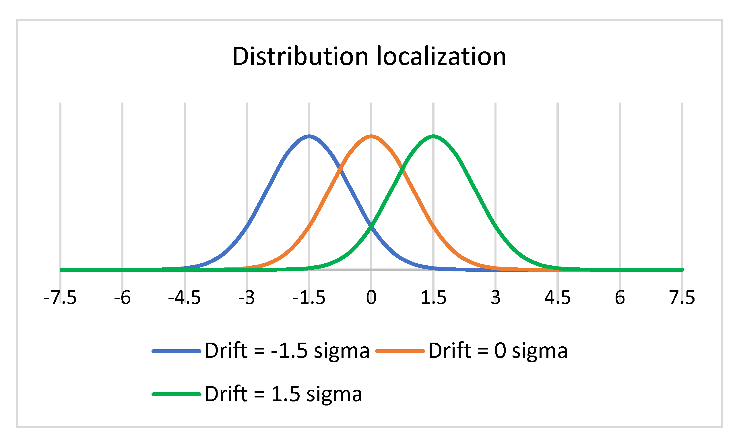
Due to this idea, Bill Smith proposed adopting a process drift of 1.5σ, shown in Figure 2. The choice of this value for the drift of the process was not scientifically argued, rather it was simply considered that the process reaches this value of the drift as a result of a possible special cause, after which the elimination of this special cause and the recentering of the process are carried out.

Later, the second promoter of the new Six Sigma concept, Michel Harry, declared the shift 1.5σ concept as the second pillar of the Six Sigma method, along with the first pillar—Six—into the phrase Six Sigma [15]. If the one who initially proposed the 1.5σ value, Bill Smith, introduced it without justifying it scientifically, Michel Harry tried to justify it in various ways [15,20]: The influence of a random error—as a “drift” that all processes experience, a statistical correction or a dynamic mean off-set. However, all these justifications are strongly contested [12,13].

As a result, the “guaranteed” process performance has now been proposed as the proportion of products for the normal process beyond the 4.5σ distance from the average (the proportion on the opposite side, beyond the 6 + 1.5 = 7.5σ distance, is tiny, which is why it is neglected): The integral Laplace function F(4.5σ) = 3.4·10⁻⁶ or 3.4 PPM. This value is accepted without reservations by most authors [21,22]. This is considered the long-term performance of the 6σ process by many authors [15,22,23].

However, it is obvious that the process does not suddenly arrive from the initial state (perfectly centered) to the limit state (deviation 1.5σ), but passes through many intermediate states.

In fact, the process evolves from the most favorable state (perfectly centered) to the most unfavorable state (when it no longer meets the conditions to be considered stable), when it intervenes to eliminate the cause that made it unstable and it will be recentered.

All these states through which the process passes are states that must be associated with the concept of short-term Six Sigma performance, while for the evaluation of long-term Six Sigma performance it is correct to take into account the distribution of all intermediate states through which the process passes.

In the paper [24] this is taken into account and a rather elaborate calculation (of integral type) is made for the deviation that leads to 3.4 PPM non-conformities, but considering that the process mean drifts in a sinusoidal (sine-wave) pattern, based on Bill Smith’s representation for the drift of 1.5σ and the animation for the distribution proposed, as justification by Michel Harry [15] but contested by Burns [13]. However, this cannot be true, because such a variation is unnatural, and it cannot be accepted for a statistical distribution.

All these considerations regarding long-term Six Sigma performance are in accordance with what is stated quite firmly [18,25,26]: One can speak of capability only when the stability of the process is ensured (and this is done with the help of the control chart), and the capability calculation is performed only in the situation when the distribution of the processed data is a normal distribution (which can be characterized by the normal law).

Since most works dedicated to the Six Sigma concept associate this concept with a maximum shift of 1.5σ and a long-term performance of 3.4 PPM or 3400 PPB [23,24,27,28,29], it is obvious that this is only a short-term situation (although it is extreme—for the maximum drift), and the following question arises: For a 6σ process (which keeps its standard deviation value unchanged over time, but which naturally has a drift over time, remaining stable), what is the proportion of long-term non-conformities (long-term performance of 6σ processes)?

The way forward to obtain an answer to this question is the summation of all possible states through which a 6σ process passes, under the conditions in which it is kept stable by using the control sheet.

Through the research presented below, a completely different result is obtained from that stated in the specialized literature, i.e., that the long-term performance of a process depends on the volume of the samples by which the stability of the process is ensured and for 6σ processes it is much better than the established value of 3400 PPB: For samples with a volume greater than or equal to 4, the performance already reaches values below 100 PPB.

The remainder of this paper is organized as follows. Section 2 explores the relationship between the proportion of non-conformities of a 6σ precision process in relation to the process deviation and to the sample size used to assure the process stability. In Section 3, the mathematical algorithm for calculating the proportion of non-conformities in the long term is built and is applied for various sizes of the sample used in the Xbar chart (for average). The conclusions are presented in the last section of the paper.

2. Materials and Methods

There is a (double) infinity of combinations for the centering and the dispersion that a process can have at a given moment, which is why it is important to establish the meaning of a 6σ process in the current study.

Thus, it is considered that the 6σ process keeps its standard deviation value unchanged over time, but it can deviate from the initial position, within the limits in which it is maintained as a stable process. This scenario can be analyzed mathematically and the result is of interest for assessing the proportion of non-conformities of a 6σ precision process in relation to the process deviation.

The other simple possibility of the evolution of the process that can be analyzed is the one in which the process remains perfectly centered, but loses its precision—this is the case that allows the determination of the inflated distribution for which PPM = 3.4.

The objective of this paper will be fulfilled by following the first scenario, but before this approach it is important to explore the second scenario as well, because the literature does not provide an answer to the exciting question: In the hypothesis that the process remains perfectly centered, how much should its dispersion increase for the percentage of non-conformities to increase from the initial value of 0.0002 PPM to the established value of 3.4 PPM?

This is another direction of evolution of the process accepted for defining long-term performance in some scientific works: The process is perfectly centered, but over time it reaches an inflated distribution [15,17]. In paper [17], the minimum C_pk is searched for, through ANOVA analysis, but it is correct to search for the inflated sigma corresponding to the value 3.4/2 = 1.7 PPM (because the distribution is perfectly centered), not for the value of 3.4 PPM, as presented in paper [15].

So, the answer will be: For the precision of the perfectly centered process, which leads to the established value of 3.4 PPM, the inverse of the Laplace function is searched for, which leads to the value 3.4·10^−6/2 = 1.7·10⁻⁶.

The result can be obtained using the tables of the Laplace function, but it is easier using the NORM.DIST function from the Microsoft Excel program through successive attempts. Following this, the result of 1.7 PPM is obtained for the variable x = −4.645:

$$NORM.DIST\left(-4.645, 0, 1, TRUE\right)=1.7\mathrm{PPM}$$

(1)

So, when the process (which is kept centered) reaches an “inflated distribution” of 6/4.645 = 1.2917 (rounded: 1.3), higher than that of the initial value σ, the proportion of non-conformities will be 3.4 PPM.

So the 3.4 PPM concept can be associated with a perfectly centered process of precision 4.645σ (with an inflated sigma 1.3 times higher than the initial one, corresponding to the 6σ process).

Exploring the first scenario (the 6σ process keeps its standard deviation value unchanged over time, but it deviates in time) demonstrates it is the most prolific. In addition, within it, the possibility of analyzing the most concrete scenario can be seen: Considering the constant precision (6σ), i.e., the “precision of the 6σ process”, it can calculate the PPM depending on the sample volume (based on the control sheet for the average, which ensures the stability of the process).

Therefore, the analysis can only be done in relation to a single criterion for tracking the stability with the control chart: Placing the process within the control limits (the other criteria, supplementary run-rules—e.g., not to be more than 9 points consecutively increasing or decreasing, or not to be above/below the average—cannot be taken into account simultaneously; an analysis based only on them is presented in the paper [20]).

It is obvious that in the long term the process evolves between the limits known from the control sheet [30,31], and when it exceeds one of them it is recentered, so the long-term performance of the process is somewhere between the situation when the performance process 6σ is perfectly centered (which means 2·0.001 PPM = 0.002 PPM) and the situation when the process is at the limit of becoming “out of control”.

The control limit should not be at a distance of ±1.5σ from the average. The distance depend on the method by which the stability of the process is monitored. As a rule, the “Xbar–Range” control sheet is used, where the limits for the average are at a distance that depends on the volume of the sample, according to Lyapunov’s theorem [31]:

$$Shif{t}_{max}=3·{\sigma }_{mean}=3·\frac{{\sigma }_x}{\sqrt{n}}=\frac{3}{\sqrt{n}}·{\sigma }_x$$

(2)

where n is sample volume.

This is the maximum shift of the process, Shift_max, or maximum drift (deviation), D_max.

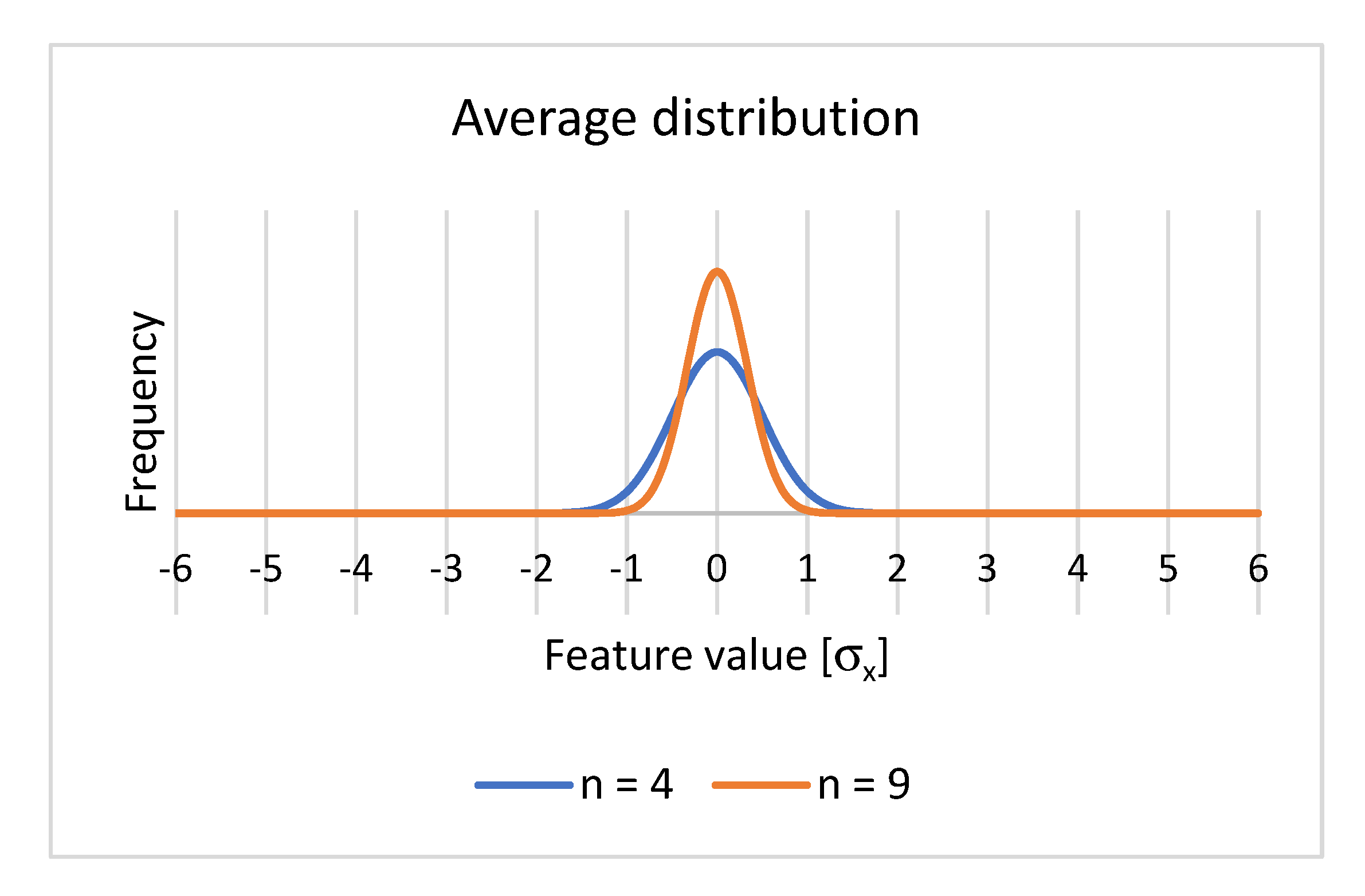
For example, the following figure shows the distribution of means for two cases (Figure 3):

• for n = 4:

$$n=4=>{\sigma }_{mean}=\frac{{\sigma }_x}{\sqrt{4}}=\frac{{\sigma }_x}{2}=>Shif{t}_{max}=3{\sigma }_{mean}=1.5{\sigma }_x$$

(3)

• for n = 9:

$$n=9=>{\sigma }_{mean}=\frac{{\sigma }_x}{\sqrt{9}}=\frac{{\sigma }_x}{3}=>Shif{t}_{max}=3{\sigma }_{mean}={\sigma }_x$$

(4)

It is known that even if the Median chart is used to ensure the stability of the processes, things are very similar [18,24,30], so the conclusions that will be obtained for the analysis performed with the Xbar chart will also be valid in the case of using other control charts.

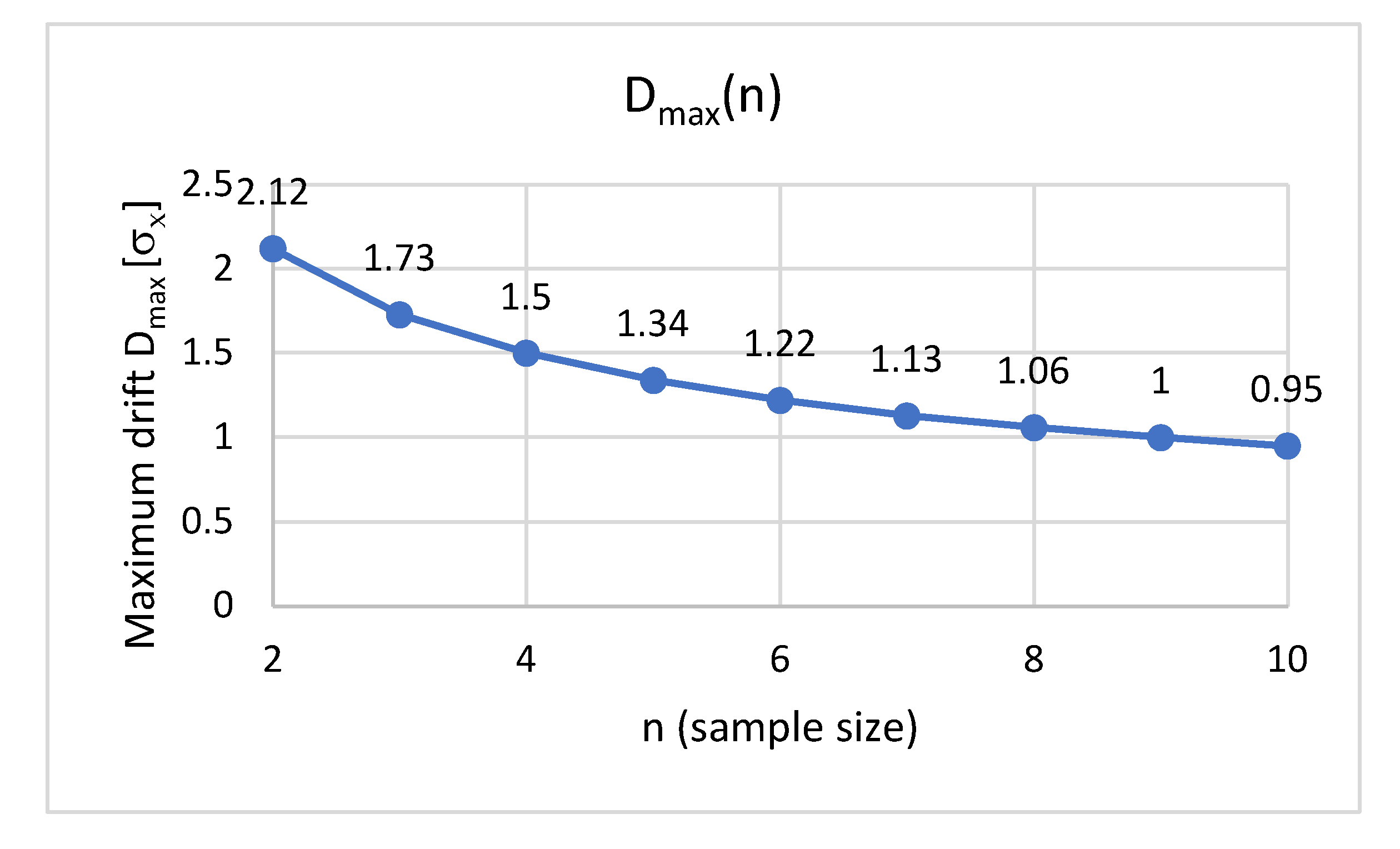
For values of the sample size n from 2 to 10, for the maximum drift (or shift) of the process, the values resulting from relation (2), expressed in σ_x units, are highlighted in Figure 4.

The graph D_max(n) reveals that the maximum deviation of the process decreases as the volume of samples used in monitoring the process increases (for example, for n = 4 it is 1.5σ_x, and for n = 9 it decreases to σ_x)—Figure 4.

Relation (2) is used in the same way by Gupta [32], who found the same values. However, the determination of these values can be done in another way. Bothe [33] takes into account sample volumes from 1 to 6, and calculates the drift value for the average at which the probability of discovering the exceeding of the control limits (thus the loss of process stability) is 0.5.

The most used indicator for evaluating the capability of a process is the capability index C_pk, because it has a simple analytical expression and is relevant enough, although there are other indicators that can characterize the capability of the process better, such as the Taguchi Capability Index, but which imply much more elaborate calculation [34].

Therefore, considering that the distribution of the data is also normal (it would not be mandatory, but so that the calculation algorithm below can be used), this being the most common situation, results in one more particularly interesting aspect: It is clear that, in any situation, the potential capability C_p will be

C_p = 12σ/6σ = 2.0,

(5)

Instead, but the capability index C_pk will depend on the drift or shift, so on the sample size being able to have values from

$$C_{pk}\equiv C_p=2.0$$

(6)

when the distribution of values is perfectly centered, up to the minimum value of

$$C_{pk,min}=\frac{6\sigma -Shif{t}_{max}}{3\sigma }=\frac{6\sigma -\frac{3}{\sqrt{n}}\sigma }{3\sigma }=2-\frac{1}{\sqrt{n}}$$

(7)

when the distribution occupies the extreme value (left or right).

So:

$$C_{pk}=\left(2-\frac{1}{\sqrt{n}}\right)\dots 2.0$$

(8)

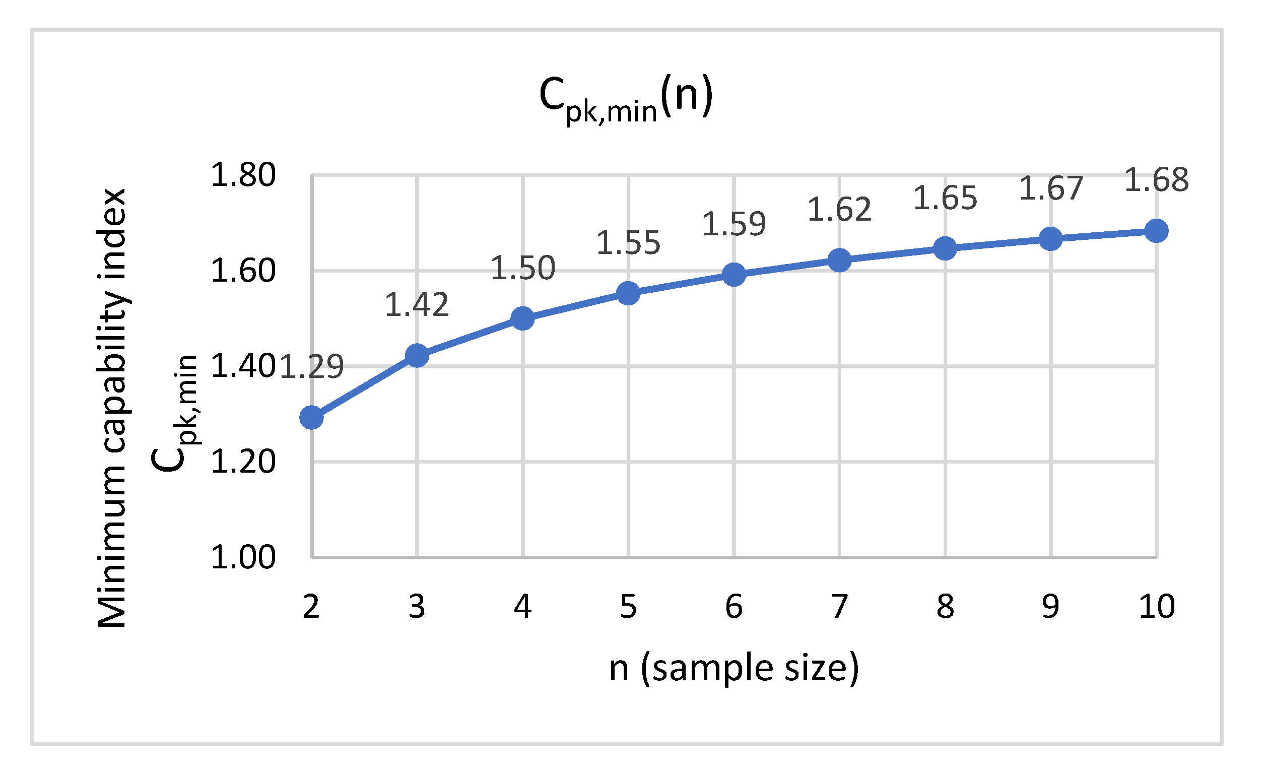
Thus, it is possible to calculate and graphically represent C_pk,min as a function of sample size n, by relation (7), for the usual values n = 2...10 (Figure 5).

In addition, in paper [33] this reasoning based on relation (7) can be found, but applied for C_p = 1.33 (when the tolerance interval is ±4σ_x) for the comparative analysis of the effective capability obtained for two values of the sample volume: n = 4 versus n = 6. In this work, C_pk,min is considered C_pk: the so-called dynamic C_pk index.

Park [20] also states that the capability is dependent on the sample volume, but he does a study not in relation to the “exceeding the control limits” criterion but in relation to the “supplementary run-rule”.

It is observed that, by increasing the volume of the sample, the increase of C_pk is obtained, and starting with volume samples 3 and 4, C_pk already exceeds the value of 1.33, generally considered as the lower limit in series production.

This means that for samples of rather small volumes (from n = 3 upwards) the Six Sigma concept “guarantees” a minimum capability above the value of C_pk = 1.33, and only in the particular case n = 4 is the well-known value of C_pk = 1.5 obtained.

Based on the central limit theorem, regardless of the distribution of the analyzed characteristic, the distribution of the sample means approaches the normal law (the more the number of data is larger).

If the characteristic distribution is considered to be normal (as it is considered within the Six Sigma method), the opportunity arises to evaluate the proportion of non-conformities depending on how the stability of the process is ensured (depending on the volume n of the samples; usually n can have values of to 2 to 10, but most frequently n = 3, 4 or 5), according to the algorithm presented below.

3. Results

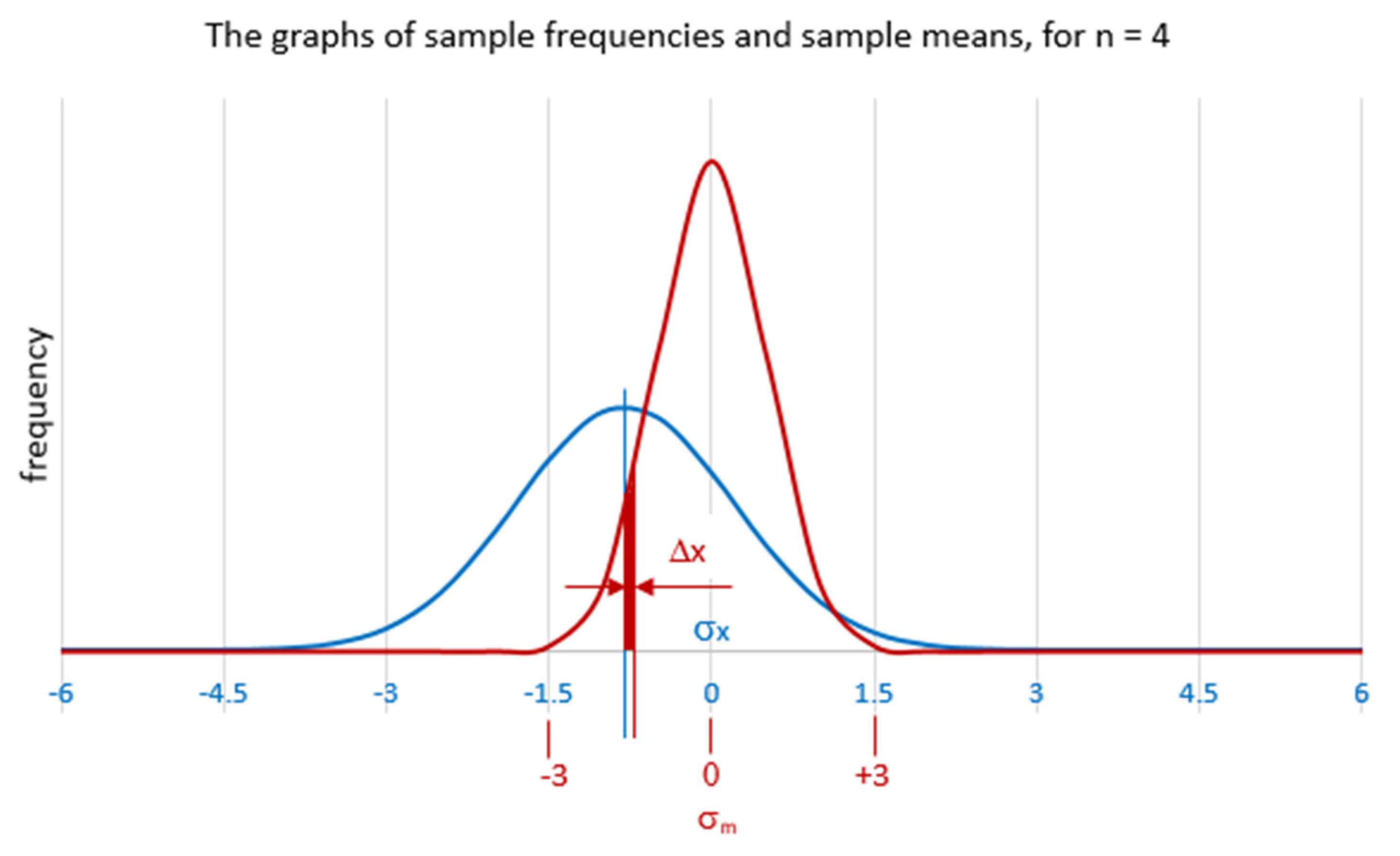
The distribution of the mean is considered within the range of $\pm 3{\sigma }_{\overline{X}}$ compared with the mean of the means $\stackrel{=}{X}$ (as is worked out on the control sheet for the mean, where the control limits are, according to the 3 sigma rule, at a distance of $\pm 3{\sigma }_{\overline{X}}$ compared with the mean), with ${\sigma }_{\overline{X}}=\frac{{\sigma }_x}{\sqrt{n}}$, where n is the sample size (according to Lyapunov’s theorem [31]).

The distribution is centered ($\stackrel{=}{X}$ is identical to half of the tolerance range $\pm 6{\sigma }_x$), with ${\sigma }_{\overline{X}}=\frac{{\sigma }_x}{\sqrt{n}}$, where n is the sample size. In Figure 6, it is exemplified for the case of volume samples n = 4, when ${\sigma }_{\overline{X}}\left(n=4\right)=\frac{{\sigma }_x}{\sqrt{4} }=\frac{{\sigma }_x}{2 }$.

Our study takes into account the normed normal law: The number of steps m is adopted and the domain of definition of the normed normal distribution for the mean (−3, 0) is discretized with the corresponding working step, ∆x = 3/m, and the calculation will be made for half of the domain of definition, given that the normal function is symmetric, so the result obtained must finally be multiplied by 2.

In order to cover the entire theoretical domain of definition (−∞, 0), which represents 50% of the distribution, (1 + m) steps are used: Thus, for i = 0 … m, the values are calculated:

$$x_i=-3+i·\frac{3}{m}=-3\left(1-\frac{i}{m}\right), i=0\dots m,$$

(9)

for which the corresponding Laplace integral function is calculated (the area under the f(x) curve to the left of each x_i value) using the NORM.DIST function available in the Microsoft Excel software:

$$F\left(x_i\right)=NORM.DIST\left(x_i, 0, 1, \mathrm{TRUE}\right), i=1\dots m,$$

(10)

and for i = 0 the value will be considered $F\left(x_0\right)=0$.

The area of each surface element of width ∆x under the mean distribution graph (see Figure 6) will be calculated with the relation:

$$A_{element,i}=F\left(x_{i+1}\right)-F\left(x_i\right), i=0\dots m$$

(11)

As for a certain sample size n, between the mean square deviation of the mean of the samples σ_m and the mean square deviation of the analyzed characteristic σ_x, there is the relationship:

$${\sigma }_m=\frac{{\sigma }_x}{\sqrt{n}}$$

(12)

If the notation is used

$$k=\frac{3}{\sqrt{n}}$$

(13)

the distances from the tolerance limits (ie ± 6σ_x) of these surface elements of the media distribution will be:

• the distance to the near limit, on the left (−6σ_x):

$$d_{l,i}=\left(6-\frac{3}{\sqrt{n}}\right)+i·∆\mathrm{x}=\left(6-\mathrm{k}\right)+\mathrm{i}·\frac{\mathrm{k}}{m}$$

(14)

• the distance from the far limit, on the right (+6σ_x):

$$d_{r,i}=12-d_l$$

(14′)

The proportion of non-conformities (values beyond ±6σ_x limits) corresponding to the two distances consists of the following two “queues”:

$$Q_{l,i}=1-\mathrm{NORM}.\mathrm{DIST}\left(d_{l,i}, 0, 1, \mathrm{TRUE}\right)$$

(15)

$$Q_{r,i}=1-\mathrm{NORM}.\mathrm{DIST}\left(d_{r,i}, 0, 1, \mathrm{TRUE}\right)$$

(15′)

As a result, for a surface element of the distribution of means (slice), the proportion of non-conformities (values beyond the ±6σ_x limits) will be proportional to the area under the mean frequency curve $f\left(\overline{X}\right)$ for that element:

1—values smaller than −6σ_x (the near limit, on the left):

$$P_{l,i}=A_{element,i}·Q_{l,i}$$

(16)

2—values greater than 6σ_x (the far limit, on the right):

$$P_{r,i}=A_{element,i}·Q_{r,i}$$

(16′)

For the respective surface element, the proportion of non-conformities will be the sum:

$$P_{element,i}=P_{l,i}+P_{r,i}$$

(17)

For half of the normal distribution of the mean, the total proportion of non-conformities is obtained by summing the (1 + m) calculation elements, and for the entire distribution (which is a symmetric distribution) the amount obtained is doubled, i.e.:

$$P_x=2·{\displaystyle \sum }_i{P}_{element,i}$$

(18)

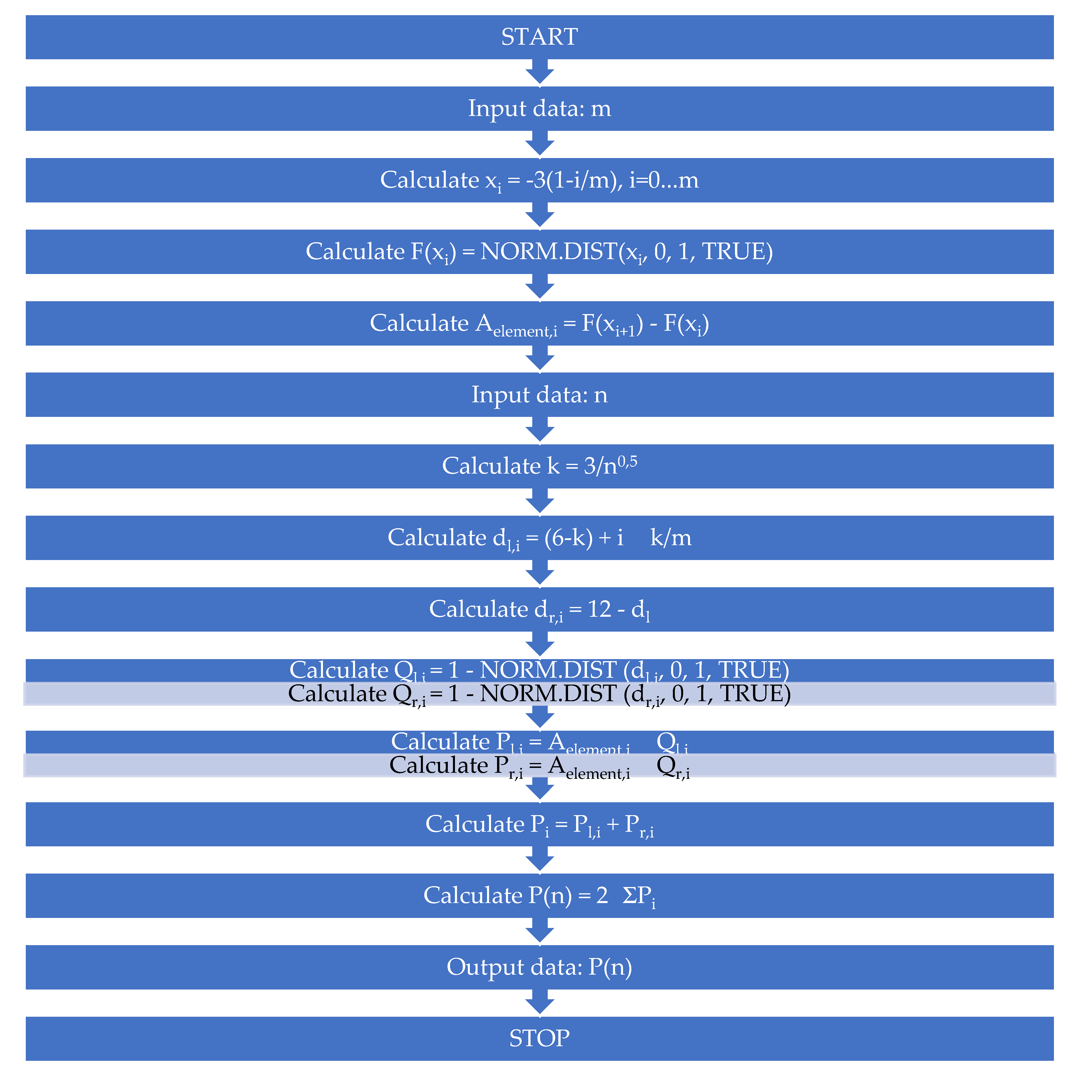
Using the facilities of the Microsoft Excel program, the calculation was made for each size n of the sample, n = 2 … 10, for a certain predetermined work step, according to the following logical scheme (Figure 7):

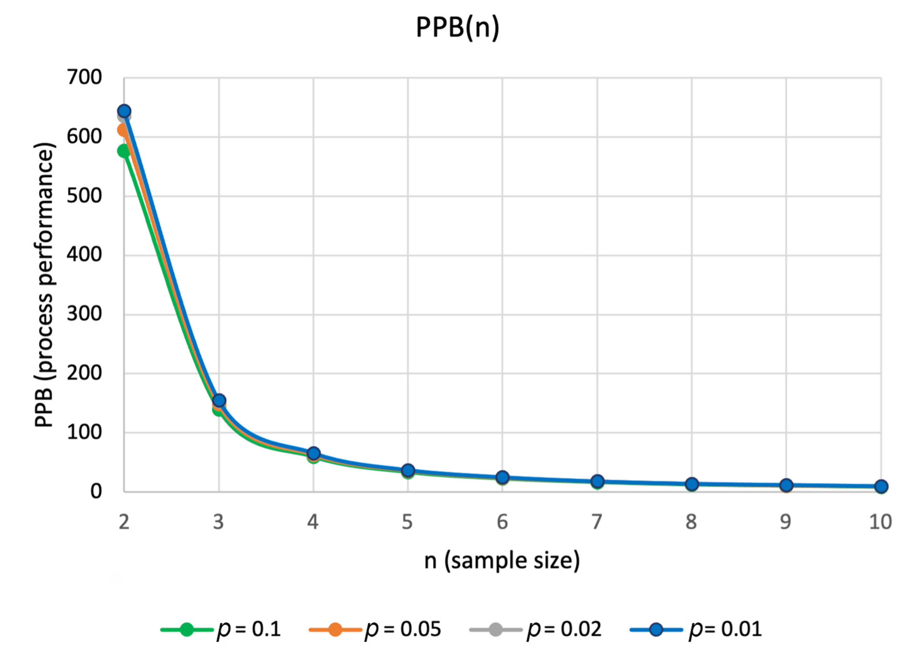
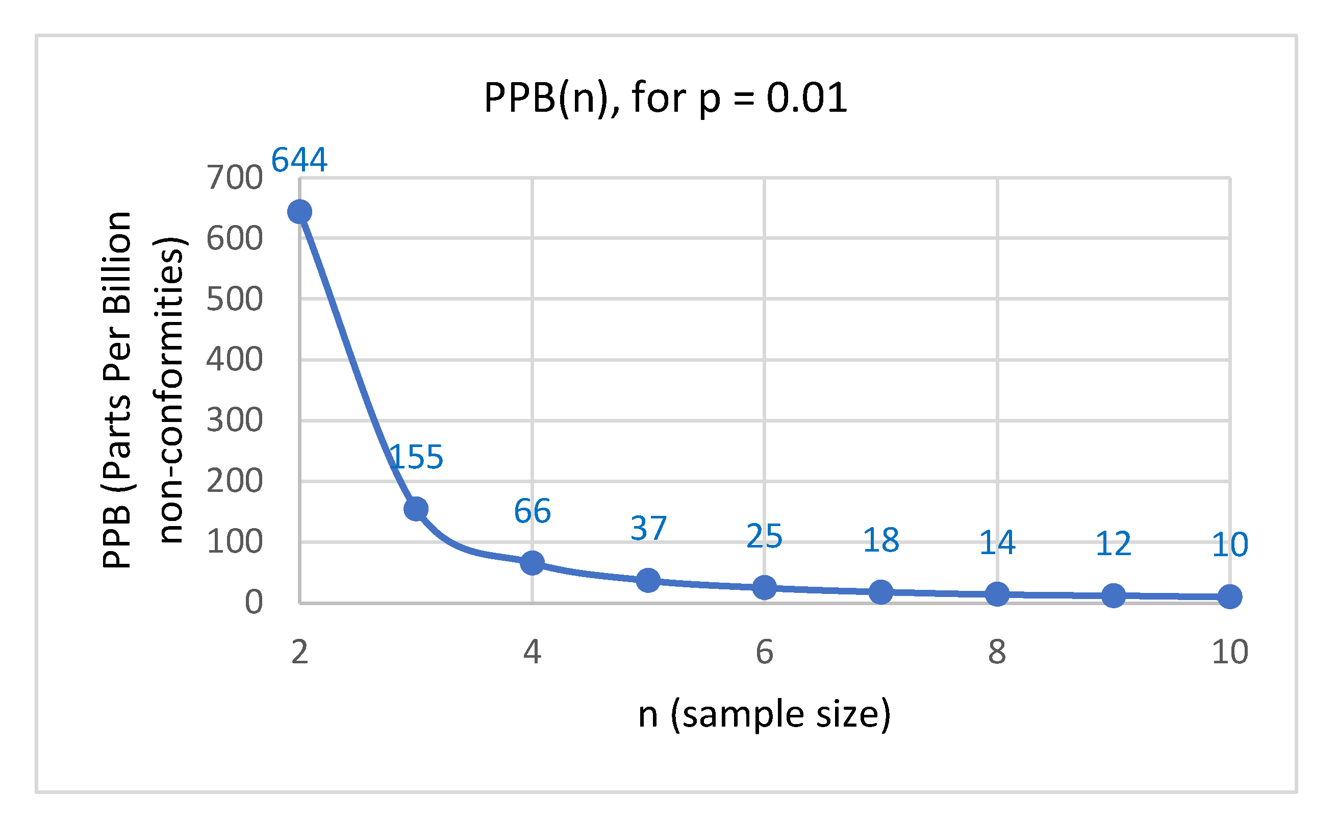
The final results obtained for the finest work steps (0.1; 0.05; 0.02; 0.01), to obtain the smallest surface elements, are presented in

Table 1. The values for parts per billion, for n = 2 … 10, obtained for different work steps.

Sample Size, n	Proportion of Non-Conformities
	Step = 0.1 (30 + 1) Steps		Step = 0.05 (60 + 1) Steps		Step = 0.02 (150 + 1) Steps		Step = 0.01 (300 + 1) Steps
	Per Units	PPB	Per Units	PPB	Per Units	PPB	Per Units	PPB
2	5.77081 × 10−7	577	6.13154 × 10−7	613	6.36392 × 10−7	636	6.44419 × 10−7	644
3	1.39784 × 10−7	140	1.47967 × 10−7	148	1.53206 × 10−7	153	1.5501 × 10−7	155
4	6.00674 × 10−8	60	6.336 × 10−8	63	6.54582 × 10−8	65	6.6179 × 10−8	66
5	3.41757 × 10−8	34	3.5932 × 10−8	36	3.70472 × 10−8	37	3.74297 × 10−8	37
6	2.28138 × 10−8	23	2.3915 × 10−8	24	2.46124 × 10−8	25	2.48513 × 10−8	25
7	1.68319 × 10−8	17	1.75967 × 10−8	18	1.808 × 10−8	18	1.82454 × 10−8	18
8	1.32781 × 10−8	13	1.38474 × 10−8	14	1.42065 × 10−8	14	1.43293 × 10−8	14
9	1.0979 × 10−8	11	1.14242 × 10−8	11	1.17046 × 10−8	12	1.18004 × 10−8	12
10	9.39479 × 10−9	9	9.7559 × 10−9	10	9.9831 × 10−9	10	1.00607 × 10−8	10

(where the proportion of non-conformities parts per billion (PPB) has been rounded to the nearest whole number) and are graphically represented in Figure 8.

Before interpreting the obtained results, it is necessary to evaluate how much the step used matters for the accuracy of the calculations.

The working method, of course, has an inherent error, given by the fact that the discretization domain of the sample means was limited to ±3 compared with the mean for the normalized normal distribution, and by the limitation of the number of steps (the finest discretization was for 300 steps).

Analyzing the data in Table 1 and the four graphs in Figure 8, it was found that, for these reduced values of the step, relatively small different values were obtained, which means that at this level of detail the errors of the method are acceptable, and, therefore, the results obtained for the smallest step (0.01) will be used for interpretation (Figure 9).

It was found that, by increasing the fineness of the step, not much was gained in the precision aspect, so the values obtained with the finest step, of 0.01, came close enough to the exact values that would result from integral calculation, so the conclusions that are formulated are absolutely justified in this regard.

The obtained results will not change significantly for a finer step, so conclusions can be formulated based on the values obtained for the finest step and represented in Figure 9.

It is obvious that the results obtained are significantly different from the value of 3400 PPB, which is accepted by most authors [15,23,24,27,28,29] or disputed by other authors [11,12,13] who do not propose another solution.

It is very interesting that, in order to obtain a substantial increase in long-term capability, it is effective to use not very large samples: Following the graph in Figure 9, it can be stated that the most recommended is the sample of size n = 4, which leads at a long-term capability below 100 PPB (and by no means known value of 3400 PPB).

Better values were found for the long-term performance of the 6σ process as larger volume of samples were used to ensure the stability of the process.

4. Conclusions

It is found that, for 6σ processes, two long-term scenarios can be analyzed:

• the precision of the process is maintained at the level of 6σ, but over time a drift of the process occurs, which can reach values that depend on the volume of the sample used in the control sheet through which the stability of the process is monitored;
• the process remains perfectly centered, but the standard deviation increases over time (inflated distribution); in this case, the 3.4 PPM level is obtained for an increase of 1.3 times the standard deviation, and the tolerance limits (both) are reached at distances of 4.645σ_inflated.

Exploring the first scenario (the 6σ process keeps its standard deviation value unchanged over time, but it deviates in time) is the most prolific, so that the main research followed this path.

The results obtained regarding the maximum drift Shift_max and the capability, characterized by the C_pk index, are in accordance with what other authors have studied (they have values that depend on the volume of the sample), but they are presented in a very clear way and for a wide range of values of the sample size, both as analytical relations and as graphic representations.

Our contribution is the fact that the following original statement is argued: It is true that, by ensuring the stability of the process by using the control sheet for the average, the process can reach a maximum drift of Shift_max = $\frac{3}{\sqrt{n}}$, but this is not the long-term performance of the process—it is still a short-term performance, the lowest, at the time when the adjustment will intervene and the process will be recentered, which will have the best short-term performance at this moment.

It was also highlighted that by using only one of the criteria for monitoring stability through the Xbar chart (the one that appears most frequently and can be exploited mathematically: The appearance of values outside the control limits, without taking into account the supplementary run-rules), a minimum value can be calculated for the long-term performance of a process depending on the volume of samples used for the control sheet.

The main conclusion resulting from the calculations is that, in the case of a 6σ process, the long-term performance is better than the established value of 3400 PPB: For small volume samples, of two pieces, it is below 700 PPB; for three pieces it is below 200 PPB; and for samples with a volume greater than or equal to four the performance already reaches values below 100 PPB.

Moreover, these values, obtained only on the basis of a single stability monitoring criterion (exceeding the control limits), are coverage values, i.e., the performance of the 6σ processes is definitely even better. Thus, for the most common case, which is associated with a 1.5σ shift (when the sample volume is n = 4) and a value of 3400 PPB, with certainty for the 6σ process the proportion of non-conformities is below 100 PPB.

The research was based on only one criterion for evaluating the stability of the 6σ processes, although the most important one—exceeding the control limits for the average. The most promising direction for research development is the simultaneous consideration of several process stability evaluation criteria, which will surely lead to even better values for long-term performance of 6σ processes.

These results obtained in the current research will further motivate the researchers and practitioners in the field of quality to consider keeping the stability of the processes under control as a priority, along with ensuring the highest possible precision of the process.