Article

Groundwater Management Based on Time Series and Ensembles of Machine Learning

by
Khalaf Okab Alsalem
1,
Mahmood A. Mahmood
1,2,
Nesrine A. Azim
2 and
A. A. Abd El-Aziz
1,2,*
1
Department of Information Systems, College of Computer and Information Sciences, Jouf University, Sakakah 72388, Saudi Arabia
2
Department of Information Systems and Technology, Faculty of Graduate Studies for Statistical Research, Cairo University, Giza 12613, Egypt
*
Author to whom correspondence should be addressed.
Processes 2023, 11(3), 761; https://doi.org/10.3390/pr11030761
Submission received: 13 February 2023 / Revised: 28 February 2023 / Accepted: 2 March 2023 / Published: 4 March 2023

Abstract

:
Due to the necessity of effective water management, the issue of water scarcity has developed into a significant global issue. One way to collect water is through the water management method. The most common source of fresh water anywhere in the world is groundwater, which has developed into a significant global issue. Our previous research used machine learning (ML) for training models to classify groundwater quality. However, in this study, we used the time series and ensemble methods to propose a hybrid technique to enhance the multiclassification of groundwater quality. The proposed technique distinguishes between excellent drinking water, good drinking water, poor irrigation water, and very poor irrigation water. In this research, we used the GEOTHERM dataset, and we pre-processed it by replacing the missing and null values, solving the sparsity problem with our recommender system, which was previously proposed, and applying the synthetic minority oversampling technique (SMOTE). Moreover, we used the Pearson correlation coefficient (PCC) feature selection technique to select the relevant attributes. The dataset was divided into a training set (75%) and a testing set (25%). The time-series algorithm was used in the training phase to learn the four ensemble techniques (random forest (RF), gradient boosting, AdaBoost, and bagging. The four ensemble methods were used in the testing phase to validate the proposed hybrid technique. The experimental results showed that the RF algorithm outperformed the common ensemble methods in terms of multiclassification average precision, recall, disc similarity coefficient (DSC), and accuracy for the groundwater dataset by approximately 98%, 89.25%, 93%, and 95%, respectively. As a result, the evaluation of the proposed model revealed that, compared to other recent models, it produces unmatched tuning-based perception results.

1. Introduction

Water is a common resource that benefits everyone—people, animals, plants, and grass. It is also a major aspect of government assistance and individual well-being. Every part of the body receives oxygen from the water the lungs supply. Water preserves a significant portion of the human body and maintains a constant internal temperature. Water covers more than 70% of the planet, including seawater, with 1.7% being groundwater. Groundwater accounts for approximately 33% of global freshwater withdrawals and handles the greatest amount of open freshwater [1].
Groundwater and other sources provide fresh water for drinking, irrigation, and industrial processes. Subsurface water, or groundwater, is the freshwater found in the pore space of stones and soil. Approximately 790 billion cubic meters of water seep into the soil, and it is anticipated that approximately 430 billion cubic meters will remain in the top layers of the soil, producing the soil moisture required for vegetation growth. The remaining 360 billion cubic meters percolate in the porous strata and show the actual enrichment of groundwater. Only 255 cubic billion meters of water can be extracted economically from this [1].
As a result, sustainable groundwater management significantly impacts a nation’s overall growth. In many nations worldwide, it has become abundantly clear in recent decades that groundwater is one of the most valuable natural resources. Compared to surface water, groundwater has many significant advantages: it is typically of higher quality, is better protected from infectious agents and other potential contaminants, is less susceptible to seasonal and perennial variation, and is much more evenly distributed across vast areas than surface water. Groundwater is frequently available where surface water is scarce [2].
Groundwater well fields can be added gradually to meet the water demand, whereas hydro-technical facilities for the use of surface water also require significant one-time investments. Groundwater is the only source of water supply for some nations, including Saudi Arabia, Malta, and Denmark. It is the most significant component of other nations’ total water supply. Tunisia uses 83% groundwater, Belgium uses 75%, and the Netherlands, Germany, and Morocco use 70% groundwater. Most European nations, including Austria, Belgium, Denmark, Hungary, Romania, and Switzerland, use more than 70% of their total water supply. In countries with arid or semiarid climates, groundwater is frequently used for irrigation. Groundwater is used to irrigate about a third of the landmass. Groundwater irrigates 45% of the irrigated land in the United States, 58% in Iran, and 67% in Algeria, and irrigated agriculture in Libya is entirely dependent on high-quality groundwater [3].
Anthropogenic activities such as farming creation, mechanical development, urbanization with increasing misuse of water assets, and common procedures such as geography, groundwater development, energized water quality, soil/rock collaborations with water, and air input can all have an impact on the nature of water [4]. Groundwater quality is still a fundamental issue, and the groundwater quality assessment is typically expected to adequately comprehend and address the springs [5]. The numerous alluvial aquifers are more susceptible to pollution-related activities due to increased groundwater extraction [6,7]. The contamination makes it difficult to obtain water from the land. Using groundwater from aquifers deep in the earth depletes water sources that take hundreds of years to collect [8].
Nations can experience water scarcity if they have low groundwater levels, irregular rainfall, and high evaporation rates caused by extremely high temperatures. According to the 2012 World Water Assessment Program (Wwap) report by the United Nations Educational, Scientific, and Cultural Organization (UNESCO), water scarcity and overabundance are among the world’s most pressing issues. A lack of groundwater, funnel spills, and standards for providing water or circulation are the primary causes of this. Moving to a town or city also alters the carbon cycle, raises expectations for everyday conveniences, and creates unusual climate or atmospheric changes.
All nations are affected by the water shortage problem, with 1.2 billion people living in a physical and 1.6 billion in a financial shortage. According to the United Nations (2019), the financial shortfall is primarily due to districts requiring more essential steps in water foundation management.
In this research, we used ensemble techniques and a time-series algorithm to propose a hybrid technique to enhance the multiclassification of the groundwater. We used the GEOTHERM dataset and pre-processed it by replacing the missing and null values, solving the sparsity problem with our recommender system proposed in Ref. [9], and applying the SMOTE sampling technique. We used the PCC feature selection method to reduce the dataset’s dimensionality. We divided the GEOTHERM dataset into a training set (75%) and a testing set (25%). The time-series algorithm was used in the training phase to learn the ensembles (RF, gradient boosting, AdaBoost, and bagging). The four ensemble methods were used in the testing phase to validate the proposed hybrid technique. The experimental results showed that the RF time-series algorithm outperformed the common ensemble methods in terms of multiclassification average precision, recall, DSC, and accuracy by approximately 98%, 89.25%, 93%, and 95%, respectively. As a result, the evaluation of the proposed model revealed that, compared to other recent models, it produces unmatched tuning-based perception results. The following is a summary of the contributions made in this research:
  • A robust model using the time-series algorithm and four ensemble techniques was proposed to distinguish between excellent drinking water, good drinking water, poor irrigation water, and very poor irrigation water.
  • We used the GEOTHERM dataset and pre-processed it by replacing the missing and null values, solving the sparsity problem with our recommender system proposed in [9], and applying the oversampling technique SMOTE.
  • The dataset’s dimensionality was reduced by the PCC feature selection method.
  • With average precision, recall, DSC, and accuracy of approximately 98%, 89.25%, 93%, and 95%, respectively, the RF model differentiated between excellent drinking water, good drinking water, poor irrigation water, and very poor irrigation water.
The remainder of this paper is formulated as follows: Section 2 presents a literature review of groundwater classifier systems. A background on feature selection, time-series algorithms, and ensemble techniques is given in Section 3. Section 4 displays the proposed model’s methodology, the dataset’s pre-processing, and the learning of the four ensembles. The findings are presented and discussed in Section 5. The research’s conclusion and future works are outlined in Section 6.

2. Literature Review

Ref. [10], the Drinking Water Quality Early Warning and Control Framework (DEWS), was created to meet China’s urgent need for safe drinking water in urban areas. The DEWS has a web administration structure and offers clients water quality monitoring, early warning, and dynamic disaster monitoring capabilities. Based on the criticism of the control of urban water frameworks, the standards of control hypothesis and hazard evaluation served as the basis for the DEWS’s usefulness. Regarding water quality early warning and crisis dynamics, the DEWS was implemented in a few large Chinese urban communities and performed well. The proposed framework links together water health theories and technologies.
Ref. [11] outlined a novel framework for observing and anticipating the quality of water using the following unique systems. Andromeda refers to ocean waters, and inter-risk refers to surface air and fresh waters. A fuzzy expert framework was utilized to provide early warnings when a particular ecological boundary exceeded certain contamination limits. In addition, to avoid unfortunate natural occurrences, ML and adaptive filtering techniques were utilized one day ahead of expectations for specific water quality boundaries.
Ref. [12] proposed a fitness value and a neural-network-based intelligent system composed of genetic tasks for model preparation. For water collection and distribution, the fitness method was used to create new intelligent individuals from the existing population of water resources. The framework is important for water use and decision-making techniques to increase development efficiency by determining the target capacities of different types of people. The proposed model also selected the attributes that affect the decision label using the feature selection method.
Four factors were considered in Ref. [13]: pH, TDS, latitude, and longitude. Two methods for multivariate group analysis used latitude and longitude to spatially partition the groundwater quality in Madinah, Western Saudi Arabia. The results showed that the two unsupervised ML methods (k mean and k medoids) produced generally similar results when the study area was divided into three primary locations with different designs: southwest, southeast, and north. Because it is an effective fact-gathering tool for water quality boundaries, the study demonstrated that multivariate bunch investigation could provide useful data for water quality management.
Unsupervised ML was used in Ref. [14] to identify oddities in cyber–physical systems (CPSs). The approach was examined and compared to a one-class SVM. The authors proposed a deep neural network (DNN) that could be applied to time-series data and implemented a probabilistic anomaly indicator. These methods were considered and contrasted with the information from Secure Water Treatment (SWaT), a smaller but still fully operational crude water sanitization plant.
Ref. [15] proposed a healthcare recommendation system by utilizing ML algorithms to recognize water-influenced habitations. The authors used recommender systems to characterize the water-influenced residences and give important suggestions.
Ref. [16] proposed a simple tool for groundwater quality classification based on many different constituents. Hierarchical clustering analysis (HCA) and a classification and regression tree (CART) were utilized to implement the tool and create groundwater quality classes. There are 10 factors used as inputs to the tool. This tool could be used as a groundwater quality identifier before building new water supplies; adding extra groundwater quality parameters will enhance the outcomes. The tool could likewise be utilized for prioritizing the groundwater quality areas, and its legitimacy can be evaluated by arranging a detailed spatial and temporal analysis of the groundwater quality in the equivalent area or another area. The outputs of the tool were the groundwater quality classes.
Using the four traditional water facies diagrams, in Ref. [17], researchers assessed groundwater quality in the northern and western regions of Saudi Arabia. The authors used stochastic geostatistics to determine the spatial distribution of various significant components in the groundwater of the Tabuk-Madina zone and principal component analysis (PCA) to identify the elements that control the chemistry of the groundwater.
Ref. [18] presented a study on groundwater quality, pollution sources, various groundwater quality, and spatial circulation. Groundwater bodies and an agent-observing network that makes it possible to determine the chemical status of groundwater bodies are the reasons for evaluating groundwater quality. In the research facility, the water samples were tested for four physicochemical factors using standard methods and compared to the principles.
Ref. [19] divided Riyadh’s Saudi Arabian governorate into five areas to assess drinking water quality: the Riyadh primary zone, Ulia, Nassim, Shifa, and Badiah. The primary water network and the underground and upper household tanks comprise the water collected in each location. A mathematical approach known as the “water quality index” (WQI) was utilized to simplify the explanation of water quality. Four physicochemical and microbial factors were used to calculate the WQI. According to the findings of this study, all of the examined water samples’ densities of heavy components were found to be within safe cutoff points. The results also revealed that the main area of Riyadh had the highest absolute number of microbes, followed by the Ulia, Albadyah, Shifa, and Alnassim zones.
Ref. [20] compared the quality levels of water from various brands of bottled drinking water (BDW) used in KSA to the BDW standards. The authors used seven factors to evaluate BDW’s quality.
From the previous review of recent studies, we can conclude that many researchers are attempting to solve the classification problem of potable groundwater. With the GEO-THERM dataset, our proposed RF model achieved an average precision, recall, DSC, and accuracy of 98%, 89.25%, 93%, and 95%, respectively.

3. Background

3.1. Ensemble

An ML ensemble consists of only a concrete, finite set of alternative models but typically allows for a much more flexible structure among those alternatives. In contrast to a statistical ensemble in statistical mechanics, which is typically infinite, ensemble methods in statistics and ML use multiple learning algorithms to obtain better predictive performance than could be obtained from any of the constituent learning algorithms alone [21,22,23].
A general meta-method of ML, ensemble learning aims to improve predictive performance by combining predictions from multiple models. There are three main approaches to ensemble learning, even though the number of ensembles that can be created for a predictive modeling problem appears to be infinite. Each field of study has produced numerous methods that are more specialized than the algorithms. Bagging, stacking, and boosting are the three main types of ensemble learning methods.

3.1.1. Bagging

The bagging method, also referred to as bootstrapping aggregation, is an algorithm that is entirely dependent on the data. From the actual dataset, multiple small subsets of data are created. By adjusting the stochastic distribution of the training datasets, bagging aims to produce more diverse predictive models in which minor changes in the training data set will significantly alter model predictions and boost their accuracy, as shown in Figure 1. It does this by fitting either a classifier (for classification) or a regressor (for regression). It has been used with decision stumps, artificial neural networks (ANNs) (including multilayer perceptrons), support vector machines, and maximum entropy classifiers, among other ML algorithms. Combining bootstrapping (sampling technique) and aggregation is called “bagging”. Bootstrapping-trained ensemble models replicate the training dataset. The majority vote of the model’s predictions, or regression averaging, is used in aggregation to arrive at the final prediction. The predictions made by each classifier or regression model are combined with the final predictor, also known as a bagging classifier. The advantage of bagging is that it reduces variance, which prevents overfitting. It also works well with data with many dimensions. Bagging has the disadvantages of being computationally expensive, having a high bias, and reducing a model’s interpretability. A good example of bagging is the RF algorithm. Implementing the bagging method can be difficult due to the following issues: determining the maximum number of bootstrap samples per subset and the best number of base learners and subsets [24].

3.1.2. Boosting

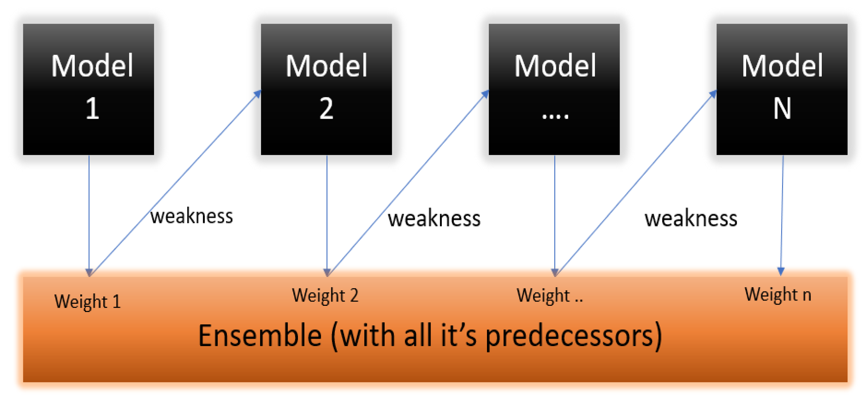
Each subsequent model tries to fix the previous model’s mistakes during boosting. Boosting is a highly adaptive method of sequentially multiple weak learners in which each model is fitted. It gives more weight to the dataset’s observations than the models in the previous sequences, as shown in Figure 2. Similar to bagging, boosting can be utilized for classification and regression problems. Adaptive boosting (AdaBoost) [26], stochastic gradient boosting (SGB) [27], and extreme gradient boosting (XGB), also known as XGBoost [28], are the three types of boost algorithms. In an ML ensemble, boosting helps reduce variance and bias and makes the model easier to understand. The fact that each classifier must correct errors in its predecessors is a drawback of boosting. Scaling sequential training in boosting is one of several obstacles that must be overcome before boosting can be implemented. As the number of iterations increases, it becomes more susceptible to overfitting and incurs additional computational costs. Last but not least, considering that the model’s behavior can be affected by many parameters, boosting algorithms can take longer to train than bagging algorithms [24].

3.1.3. Stacking

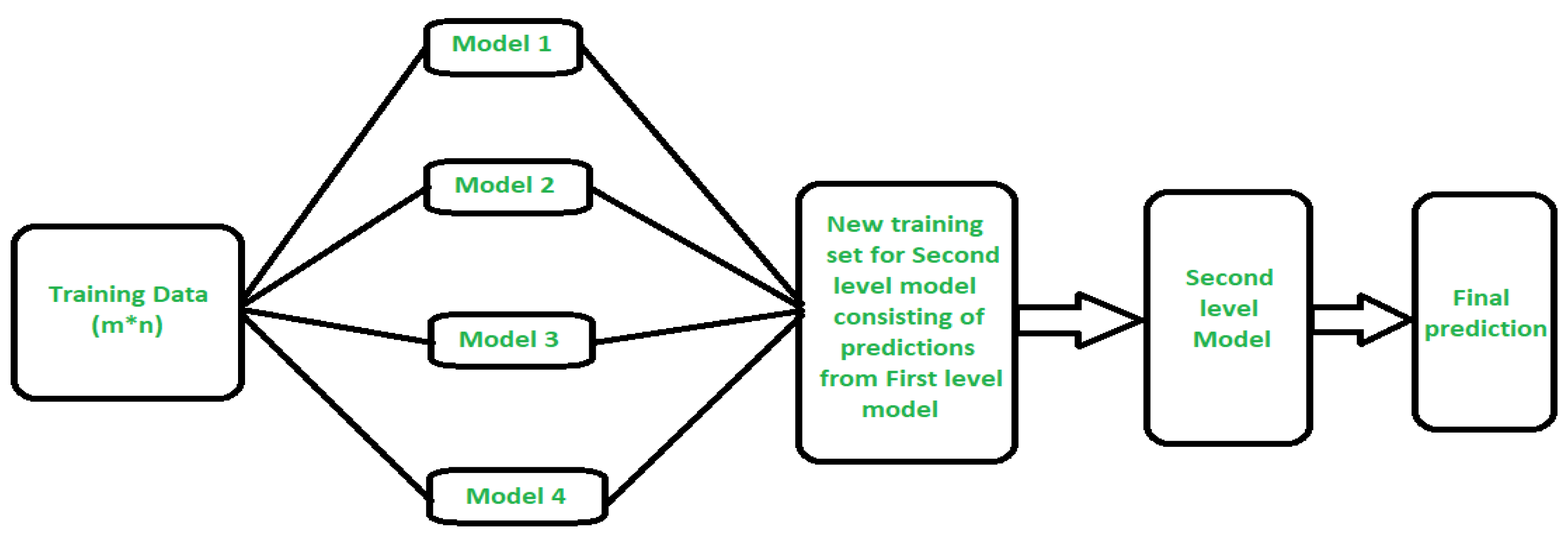
The model ensembling technique is known as the “stacking method” or “stacked generalization” and combines data from multiple predictive models to create a new model (meta-model). A stacking model’s architecture consists of two or more base models, or level 0 models, and a meta-model, or level 1 model, that combines the predictions of the base models, as shown in Figure 3. Models compatible with the training data and whose predictions are compiled make up level 0 models (base models). However, the model learns the best way to combine the predictions of the base models in the level 1 model (meta-model). Probability values or class labels may be the outputs from the base models used as inputs for the meta-model in the case of classification.
In most cases, the stacking approach outperforms all trained models. The benefit of stacking is a deeper comprehension of the data, which makes it more precise and efficient. With model stacking, so many predictors predict the same merged target that overfitting is a significant problem. Additionally, multilevel stacking is time-consuming and costly for the data due to the large amount of data required for training [24,29]. When designing a stacking ensemble from scratch, determining the appropriate number of baseline models and the baseline models that can be relied upon to generate better predictions from datasets are two challenges associated with implementing stacking. When the amount of data that is accessible increases exponentially, it also increases the difficulty of interpreting the final model and the complexity of the computation time [24].

3.1.4. Time Series

Time-series classification uses supervised machine learning to analyze multiple labeled classes of time-series data to predict or classify the class that new data belong to. This is crucial in many situations where financial or sensor data analysis may be required to support a business decision. Since classification accuracy is crucial in these circumstances, data scientists put considerable effort into making their time-series classifiers as accurate as possible. Time-series classification can be carried out with various algorithms, and one type may produce higher classification accuracy than others, depending on the data. Time-series classification algorithms can be divided into five categories: distance-based, interval-based, dictionary-based, frequency-based, and shapelet-based [30].
When working on a time-series classification problem, it is essential to take into account a variety of algorithms because of this. By indicating the algorithmic pipeline that produces the optimal accuracy for the input data set, using an automated platform that would rigorously explore the space of available algorithms and hyperparameters could save a significant amount of time, at least in the initial stages of exploration. It is anticipated that such platforms will soon be available with time-series classification capabilities [30].

4. Materials and Methods

4.1. Dataset Description

GEOTHERM is a computerized information system developed by the U.S. Geological Survey (USGS) to keep track of data on the geology, geochemistry, and hydrology of geothermal sites, primarily in the United States. The system was first proposed in 1974 and was used until 1983. The system used a mainframe computer, and key-punch cards were used to enter most of the data. A fairly extensive data entry form served as the basis for keypunching. Several products were published or made available to preserve the data when the GEOTHERM database was removed from the internet. These include a state-by-state listing of each record on microfiche and basic data for thermal springs and wells. As digital data, the GEOTHERM database was also submitted to the National Technical Information Service (NTIS) [31]. Table 1 shows the statistics of the GEOTHERM dataset. Groundwater is divided into the four categories using the water quality index (WQI) formula; see Equation (1).
WQI =   dissolved   calcium +   dissolved   magnesium +   dissolved   potassium +   pH   +   total   dissolved   solids .

4.2. Model Architecture and Training

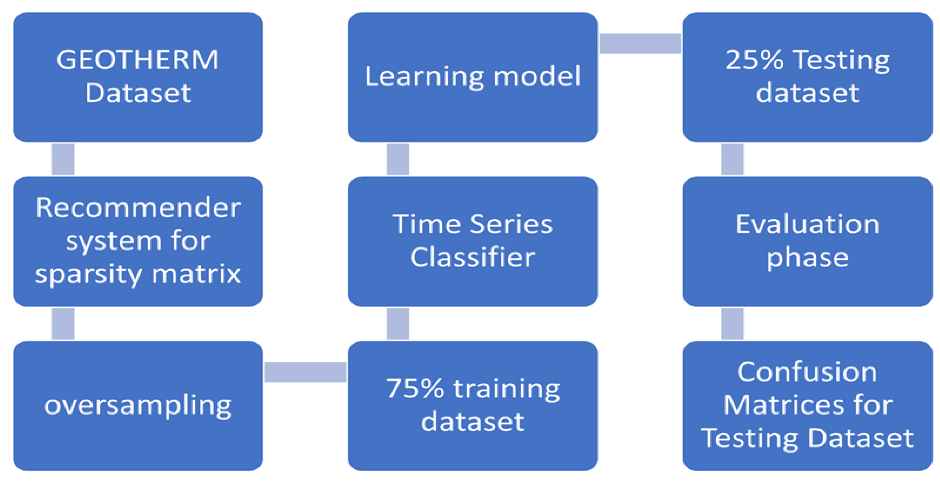
We proposed a hybrid technique composed of a time-series algorithm and four ensemble techniques. The hybrid technique used the GEOTHERM dataset to identify groundwater quality. The proposed model will be discussed in the following sections. Figure 4 describes the steps of the proposed model: (1) dataset pre-processing by replacing the missing values and replacing the null values, solving the sparsity problem, and applying the oversampling algorithm SMOTE; (2) selecting the relevant attributes of the dataset by applying the PCC technique; (3) learning the ensembles (RF, gradient boosting, AdaBoost, and bagging) using the time-series algorithm, and (4) testing and evaluating the ensemble techniques.
After downloading the GEOTHERM dataset, the proposed model proceeded with dataset pre-processing. Pre-processing the GEOTHERM datasets is one of the most crucial steps because it effectively produces accurate results. The missing values and the null values of the features of the GEOTHERM dataset were replaced by our recommender system described in Ref. [9]. Moreover, we solved the sparsity problem by using our recommender system proposed in Ref. [9] and applying the oversampling algorithm SMOTE. In addition, we used the PCC technique to reduce the dimensionality of the Geotherm dataset to the most important features. After the pre-processing phase, we divided the GEOTHERM dataset into a training set (75%) and a test set (25%). Using the time-series algorithm, we trained the four ensembles in the third step. We tested the four ensemble techniques in the four steps and calculated the measured metrics to evaluate them.

4.2.1. Data Pre-Processing

Due to data noise or missing values, the raw data may be less accurate than the final prediction. Pre-processing included replacing missing values, replacing null values, and solving the sparsity problem, which was necessary to make the data more suitable for analysis.

Missing and Null Values Handling

Missing values mean a large amount of uncertainty. We proposed a recommender system in Ref. [9]. We used it to handle the missing and null values of six features in the GEOTHERM dataset: sample date, dissolved calcium, dissolved magnesium, dissolved potassium, pH, and total dissolved solids.

Sparsity Problem

Sparse data is a common issue in ML because it affects how well algorithms work and how well they can make accurate predictions. When certain expected values in a dataset are missing, a common occurrence in large-scale data analysis, the data are considered sparse. In this research, we used the recommender systems proposed in Ref. [9] to solve the sparsity problem of the GEOTHERM dataset.

Sampling

Data sampling is a set of techniques for artificially increasing the amount of data by creating new data points or synthetic data from existing data. It can help ML models perform better and produce better results by creating new and distinct examples to train small datasets. When the dataset is extensive and sufficient, ML performs better and is more accurate. For ML models, data collection and labeling can be time-consuming and expensive processes. However, data sampling techniques can reduce these operational costs by transforming datasets.
In this research, we used the sampling technique SMOTE. Minority-class observations were classified first in this algorithm. Any minority observation was considered a noise point and was ignored when producing synthetic data if all neighbors belonged to the majority class. In addition, it only resampled from a select few border areas, which served as neighborhoods for both the majority and minority classes.
As a result of applying the SMOTE technique, the size of the GEOTHERM dataset was increased from 46,400 to 185,600. Hence, the size of the training dataset (75%) was 139,200, and the size of the test dataset (25%) was 46,400. Table 2 shows the statistics of the test data set after applying the pre-processing process.

4.2.2. Feature Selection

In machine learning and statistics, selecting the most significant attributes from a large set is known as feature selection. In ML techniques, feature selection is used before processing begins. The high-dimensional attribute space will be reduced. Feature selection has received increasing attention in recent years, and it can make the model easier to use by reducing training time [32,33].
In contrast to feature reduction techniques such as PCA, feature selection algorithms only select a limited number of attributes that are typically useful for classification and regression. As a result, feature selection is useful for understanding the relationship between attributes and locating specific internal techniques. This study used the PCC technique to select the relevant attribute from the GEOTHERM dataset. Station ID, station type, sample date, dissolved calcium, dissolved chloride, dissolved magnesium, dissolved potassium, dissolved sodium, pH, total dissolved solids, and class are the 11 features in the GEOTHERM dataset. Sample date, dissolved calcium, magnesium, potassium, pH, and total dissolved solids were the six features selected by the application of the PCC technique.

5. Model Implementation and Evaluation

5.1. Model Evaluation Metrics

The accuracy, precision, recall, and DSC described in Equations (2)–(5) were used to evaluate the proposed model.
Accuracy = (TP + TN)/(TP + TN + FP + FN)
Precision = TP/(TP + FP)
Recall = TP/(TP + FN)
DSC = (2 × TP)/(2 × TP + FP + FN)
FP, false negatives by FN, and true positives by TP represent false positives. Accuracy is the degree to which the result matches the value we aim for. Precision is calculated by dividing the total number of positive predictions by the number of true positives. The ratio of the number of actual positives to the number of true positives is the recall. The DSC is a harmonic average of precision and recall.

5.2. Model Implementation

The GEOTHERM dataset was divided into 75% for training and 25% for testing for validation in the experiment. The experiment computer has a 64-bit operating system, an x64-based processor, an Intel(R) Core (TM) i7-3612QM CPU @ 2.10 GHz and 2.1 GHz, and 10 GB RAM.
Table 3 shows the experiments’ results for the four ensembles (RF, gradient boosting, bagging, and AdaBoost), which were learned by a time-series algorithm. All four ensembles were applied to the GEOTHERM dataset for multiclassification. We distinguished between excellent drinking water, good drinking water, poor irrigation water, and very poor irrigation water. Table 3 shows that RF, gradient boosting, bagging, and AdaBoost had accuracy averages of 95%, 92%, 86%, and 79%, respectively. The RF model had the highest accuracy, precision, and DSC average at 95%, 98%, and 93%, respectively. The gradient-boosting model had the highest average recall at 91.5%. AdaBoost had the lowest accuracy, at 79%. Bagging had the lowest precision, recall, and DSC at 40.5%, 42.25%, and 41.25%, respectively.
For the excellent class, precision, recall, and DSC were 95%, 100%, and 97% for RF, respectively. RF had the highest precision and DCS, at 95% and 97%, respectively. RF and gradient boosting had the highest recall, at 100%.
For the good class, precision, recall, and DSC were 97%, 82%, and 89% for RF, respectively. Gradient boosting had the highest precision (100%), RF had the highest recall, and DSC was 82% and 89%, respectively.
For the poor class, precision, recall, and DSC were 100%, 75%, and 86% for RF, respectively. RF, gradient boosting, and AdaBoost had the highest precision (100%), while gradient boosting and AdaBoost had the highest recall and DSC at 100%.
Precision, recall, and DSC were 100% in the very poor class for RF. RF, gradient boosting, and AdaBoost had the highest precision, recall, and DSC at 100%.
Table 4, Table 5, Table 6 and Table 7 show the confusion matrices for the four ensembles. The test dataset had four classes: excellent, good, poor, and very poor. Table 4 shows that the RF model correctly predicted 34,683 samples out of 34,683 samples for the class excellent, with an accuracy of 100%. It predicted 8436 out of 10,311 samples for the class good, with an accuracy of 81%. It predicted 469 samples out of 937 samples for the class poor, with an accuracy of 50%. It predicted zero out of 469 samples for class very poor, with an accuracy of 0%.
Table 5 demonstrates that the gradient boosting model correctly predicted 34,683 of 34,683 samples for the class excellent with 100% accuracy. With an accuracy of 65.9%, it predicted 6796 out of 10,311 samples for the class good. With 100% accuracy, it correctly predicted the class poor in 937 of 937 samples. With 100% accuracy, it correctly predicted 469 of 469 samples for the class very poor.
Table 6 demonstrates that the bagging model correctly predicted 31,168 out of 34,683 samples for the excellent class with an 89.8% accuracy rate. It predicted 7265 out of 10311 samples for the class good, with an accuracy of 70%. In 469 of 937 samples, it correctly predicted the class poor with a 50% accuracy. It correctly predicted 469 out of 469 samples for the class very poor with 100% accuracy.
According to Table 7, the AdaBoost model correctly predicted 28,824 of 34,683 excellent class samples with an 83% accuracy rate. With a 63.6% accuracy, it predicted 6562 of 10,311 samples for the class good. It correctly predicted the poor class in 937 out of 937 samples with 100% accuracy. It made 100% accurate predictions for 469 of the 469 individuals in the very poor class.

6. Conclusions

This paper proposes a robust classifier to differentiate between excellent drinking water, good drinking water, poor irrigation water, and very poor irrigation water. The ensemble models serve as the basis for the classification model. In the proposed model, we used ensemble techniques and a time-series algorithm to propose a hybrid technique to enhance the multiclassification of the groundwater. The GEOTHERM dataset was used to build and evaluate the hybrid technique and pre-process it by replacing the missing and null values and solving the sparsity problem by applying the oversampling technique SMOTE. Moreover, we applied the PCC feature selection technique to select the important features. The proposed model was evaluated and compared to recent classifiers. The RF model achieved the highest precision, recall, DSC, and accuracy of 98%, 89.25%, 93%, and 95%, respectively. Consequently, the proposed RF model was evaluated and found to produce unparalleled tuning-based perception results compared to other models currently in use.

Author Contributions

Conceptualization, M.A.M. and A.A.A.E.-A.; methodology, M.A.M. and A.A.A.E.-A.; database search, data curation, assessment of bias, K.O.A. and N.A.A.; writing—original draft preparation, K.O.A. and N.A.A.; writing—review and editing, M.A.M., A.A.A.E.-A., K.O.A. and N.A.A.; supervision, A.A.A.E.-A. and M.A.M. All authors have read and agreed to the published version of the manuscript.

Funding

This work is funded through research grant no. DSR2020-03-429.

Institutional Review Board Statement

Not applicable.

Informed Consent Statement

Not applicable.

Data Availability Statement

The article contains all study-relevant data.

Acknowledgments

The authors thank the Deanship of Scientific Research at Jouf University for funding this work through research grant no. DSR2020-03-429.

Conflicts of Interest

The authors declare no conflict of interest.

References

  1. Siebert, S.; Burke, J.; Faures, J.M.; Frenken, K.; Hoogeveen, J.; Döll, P.; Portmann, F.T. Groundwater use for Irrigation: A Global Inventory. Hydrol. Earth Syst. Sci. 2010, 14, 1863–1880. [Google Scholar] [CrossRef]
  2. Menon, S. Ground Water Management: Need for Sustainable Approach; Personal RePEc Archive: Munich, Germany, 2007. [Google Scholar]
  3. Zektser, I.S.; Everett, L.G. Groundwater Resources of the World and Their Use; UNESCO Digital Library: Fontenoy, Paris, 2004. [Google Scholar]
  4. Helena, B.; Pardo, R.; Vega, M.; Barrado, E.; Fernandez, J.M.; Fernandez, L. Temporal Evolution of Ground Water Composition in an Alluvial Aquifer (pisuerga river, spain) by Principal Component Analysis. Water Resour. 2000, 34, 807–816. [Google Scholar]
  5. Mohamad, S.; Arzaneh, F.; Mohamad, J.P. Quality of Groundwater in an Area with Intensive Agricultural Activity. Expo. Health 2016, 8, 93–105. [Google Scholar]
  6. Huq, M.E.; Su, C.; Li, J.; Sarven, M.S. Arsenic Enrichment and Mobilization in the Holocene Alluvial Aquifers of Prayagpur of Southwestern Bangladesh. Int. Biodeterior. Biodegrad. 2018, 128, 186–194. [Google Scholar] [CrossRef]
  7. Huq, M.E.; Su, C.; Fahad, S.; Li, J.; Sarven, M.S.; Liu, R. Distribution and Hydrogeochemical Behavior of Arsenic Enriched Groundwater in the Sedimentary Aquifer Comparison between Datong Basin (China) and Kushtia District (Bangladesh). Environ. Sci. Pollut. Res. 2018, 25, 15830–15843. [Google Scholar] [CrossRef] [PubMed]
  8. Zaidi, F.K.; Nazzal, Y.; Ahmed, I.; Naeem, M.; Jafri, M.K. Identification of Potential Artificial Groundwater Recharge Zones in North Western Saudi Arabia Using Gis and Boolean Logic. J. Afr. Earth Sci. 2015, 111, 156–169. [Google Scholar] [CrossRef]
  9. Abd El-Aziz, A.A.; Alsalem, K.O.; Mahmood, M.A. An Intelligent Groundwater Management Recommender System. Indian J. Sci. Technol. 2021, 14, 2871–2879. [Google Scholar] [CrossRef]
  10. Hou, D.; Song, X.; Zhang, G.; Zhang, H.; Loaiciga, H. An Early Warning and Control System for Urban, Drinking Water Quality Protection: Chinas Experience. Environ. Sci. Pollut Res. 2013, 20, 4496–4508. [Google Scholar] [CrossRef]
  11. Bassiliades, N.; Antoniades, I.; Hatzikos, E.; Vlahavas, I.; Koutitas, G.; Monitoring, A.I.S.; Quality, P.W. An Intelligent System for Monitoring and Predicting Water Quality. In Proceedings of the European Conference towards eENVIRONMENT, Prague, Czech Republic, 25 March 2009; pp. 534–542. [Google Scholar]
  12. Gino Sophia, S.G.; Sharmila, V.C.; Suchitra, S.; Muthu, T.S.; Pavithra, B. Water Management using Genetic Algorithm-based Machine Learning. Soft Comput. 2020, 24, 17153–17165. [Google Scholar] [CrossRef]
  13. Alahmadi, F.S. Groundwater Quality Categorization by Unsupervised Machine Learning in Madinah. In In Proceedings of the International Geoinformatics Conference (IGC2019), Riyadh, Saudi Arabia, February 2019. [Google Scholar]
  14. Inoue, J.; Yamagata, Y.; Chen, Y.; Poskitt, C.M.; Sun, J. Anomaly Detection for a Water Treatment System Using Unsupervised Machine Learning. In Proceedings of the 2017 IEEE International Conference on Data Mining Workshops (ICDMW), New Orleans, LA, USA, 18–21 November 2017. [Google Scholar]
  15. Yuvaraj, N.; Anusha, K.; MeagaVarsha, R. Healthcare Recommendation System for Water Affected Habitations using Machine Learning Algorithms. Int. J. Pure Appl. Math. 2018, 118, 3797–3809. [Google Scholar]
  16. Adnan, S.; Iqbal, J.; Maltamo, M.; Suleman, M.B.; Shahab, A.; Valbuena, R. A Simple Approach of Groundwater Quality Analysis, Classification, and Mapping in Peshawar, Pakistan. Environments 2019, 6, 123. [Google Scholar] [CrossRef]
  17. Salman, F.K.Z.A.S.; Hussein, M.T. Evaluation of Groundwater Quality in Northern Saudi Arabia using Multivariate Analysis and Stochastic Statistics. Environ. Earth Sci. 2015, 74, 7769–7782. [Google Scholar] [CrossRef]
  18. Kamakshaiah, K.; Seshadri, R. Ground Water Quality Assessment using Data Mining Techniques. Int. J. Comput. Appl. 2013, 76, 39–45. [Google Scholar]
  19. Al-Omran, A.; Al-Barakah, F.; Altuquq, A.; Aly, A.; Nadeem, M. Drinking Water Quality Assessment and Water Quality Index of Riyadh, Saudi Arabia. Water Qual. Res. J. 2015, 50, 287–296. [Google Scholar] [CrossRef]
  20. Asma, A.K.; Al-Jaloud, A.; El-Taher, A. Quality Level of Bottled Drinking Water Consumed in Saudi Arabia. J. Environ. Sci. Technol. 2014, 7, 90–106. [Google Scholar]
  21. Opitz, D.; Maclin, R. Popular Ensemble Methods: An Empirical Study. J. Artif. Intell. Res. 1999, 11, 169–198. [Google Scholar] [CrossRef]
  22. Polikar, R. Ensemble Based Systems in Decision Making. IEEE Circuits Syst. Mag. 2006, 6, 21–45. [Google Scholar] [CrossRef]
  23. Rokach, L. Ensemble-Based Classifiers. Artif. Intell. Rev. 2010, 33, 1–39. [Google Scholar] [CrossRef]
  24. Mohammed, A.; Kora, R. A Comprehensive Review on Ensemble Deep Learning: Opportunities and Challenges. J. King Saud Univ. Comput. Inf. Sci. 2023. [Google Scholar] [CrossRef]
  25. Analytics Vidhya. Available online: https://www.analyticsvidhya.com (accessed on 1 January 2022).
  26. Freund, Y.; Iyer, R.; Schapire, R.E.; Singer, Y. An efficient boosting algorithm for combining preferences. J. Mach. Learn. Res. 2003, 4, 933–969. [Google Scholar]
  27. Friedman, J.H. Greedy function approximation: A gradient boosting machine. Ann. Stat. 2001, 29, 1189–1232. [Google Scholar] [CrossRef]
  28. Friedman, J.; Hastie, T.; Tibshirani, R. Additive logistic regression: A statistical view of boosting (with discussion and a rejoinder by the authors). Ann. Stat. 2000, 28, 337–407. [Google Scholar] [CrossRef]
  29. Ma, Z.; Wang, P.; Gao, Z.; Wang, R.; Khalighi, K. Ensemble of machine learning algorithms using the stacked generalization approach to estimate the warfarin dose. PLoS ONE 2018, 13, e0205872. [Google Scholar] [CrossRef] [PubMed]
  30. Dinger, T.; Chang, Y.C.; Pavuluri, R.; Subramanian, D. Time series representation learning with contrastive triplet selection. In Proceedings of the 5th Joint International Conference on Data Science & Management of Data, 9th ACM IKDD CODS and 27th COMAD, Bangalore, India, 7 – 10 January 2022. [Google Scholar]
  31. Goff, F.; Bergfeld, D.; Janik, C.J.; Counce, D.; Murrell, M. Geochemical Data on Waters, Gases, Scales, and Rocks. Available online: https://help.waterdata.usgs.gov/faq/additional-background (accessed on 9 November 2011).
  32. James, G.; Witten, D.; Hastie, T.; Tibshirani, R. An Introduction to Statistical Learning; Springer: Berlin/Heidelberg, Germany, 2013. [Google Scholar]
  33. Luukka, P. Feature Selection using Fuzzy Entropy Measures with Similarity Classifier. Expert Syst. Appl. 2011, 38, 4600–4607. [Google Scholar] [CrossRef]
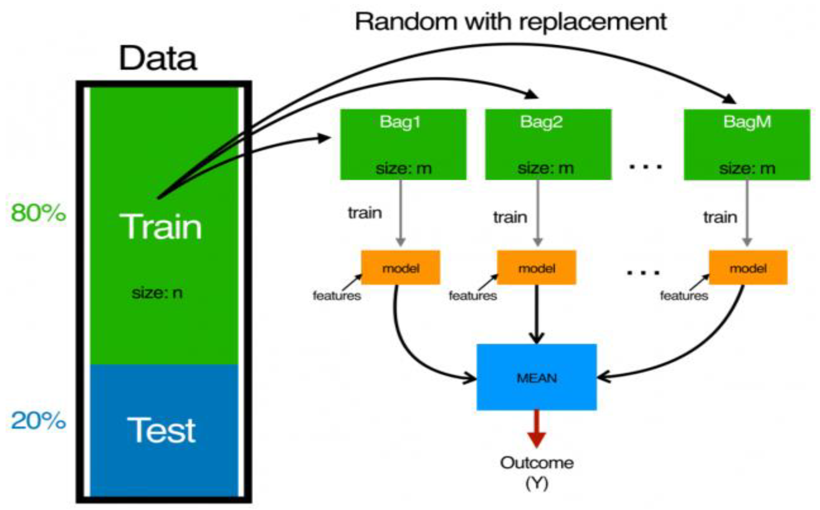
Figure 1. The bagging classifier in detail [25].
Processes 11 00761 g001
Figure 2. The boosting classifier in detail [25].
Processes 11 00761 g002
Figure 3. The stacking classifier in detail [25].
Processes 11 00761 g003
Figure 4. The architecture of the proposed model.
Processes 11 00761 g004
Table 1. The statistics of the GEOTHERM dataset.
TypeClassNo. of Rows
DrinkingExcellent34,516
Good9915
IrrigationPoor1892
Very Poor77
Total46,400
Table 2. The statistics of the GEOTHERM test dataset.
TypeClassNo. of Rows
DrinkingExcellent34,683
Good10,311
IrrigationPoor937
Very Poor469
Total46,400
Table 3. The performance of the four ensemble models using a time-series algorithm.
ModelClassPrecisionRecallDSC
RFExcellent9510097
Good978289
Poor1007586
V. poor100100100
Average 9889.2593
Accuracy95
Gradient BoostingExcellent9110095
Good1006679
Poor100100100
V. poor100100100
Average 97.791.553.4
Accuracy92
BaggingExcellent919291
Good717774
Poor000
V. poor000
Average 40.542.2541.25
Accuracy86
AdaBoostExcellent888386
Good536458
Poor100100100
V. poor100100100
Average7985.2586.7586
Table 4. The confusion matrix for RF.
1234
134,683000
21875843600
304684690
4000469
Table 5. The confusion matrix for gradient boosting.
1234
134,683000
23515679600
3009370
4000469
Table 6. The confusion matrix for bagging.
1234
131,168351500
23046726500
304684690
4004690
Table 7. The confusion matrix for AdaBoost.
1234
128,824585900
23749656200
3009370
4000469
Disclaimer/Publisher’s Note: The statements, opinions and data contained in all publications are solely those of the individual author(s) and contributor(s) and not of MDPI and/or the editor(s). MDPI and/or the editor(s) disclaim responsibility for any injury to people or property resulting from any ideas, methods, instructions or products referred to in the content.