Oil Onshore Pipeline Quantitative Risk Assessment under Fire and Explosion Scenarios

Abstract

Pipeline is one of the safest and most cost-effective means of transportation for hydrocarbons. However, hydrocarbon releases and the subsequent fires and explosions, are presented as persistent events. Quantitative Risk Assessment (QRA) enables one to address the risk and to prevent these events. In this regard, different approaches have been proposed for pipelines, but few studies are focused on oil transportation. This paper presents a methodology for performing QRA for onshore oil pipelines, which is based on the calculation of individual and societal risk indicators. This methodology is illustrated using an authentic case study of a segment of 17.53 km of the length of an onshore oil pipeline located in the southwest of Colombia, considering jet and pool fire scenarios. The results show that the Individual Risk Per Annum (IRPA) for operation (and maintenance) and administrative workers are 6.14 × 10⁻⁴ and 8.52 × 10⁻⁵ yr⁻¹, respectively. The IRPA for people close to the pipeline is between 2.31 × 10⁻⁴ and 2.60 × 10⁻⁴ yr⁻¹. The IRPA for workers is tolerable, while for people may be classified as unacceptable. The societal risk was represented using the F–N curve, indicating that risk is unacceptable and nearby populations could be relocated.

1. Introduction

Pipelines are known to be the safest and most cost-effective mode of transportation compared to trucks, trains, and ships [1] particularly when the fluids of interest are flammable, or they are subject to generating volatile organic compounds (VOC) when vented. Pipelines are subjected to different hazards throughout their life cycle, which typically results in a loss of containment (LOC). This incident may trigger undesirable events such as explosions, fires, or toxic releases, which may affect nearby people, the environment, and facilities. Although these accidents occur with relatively low frequency, the consequences could be catastrophic, considering that large volumes of hydrocarbons are often transported via these systems [2,3]. For instance, a statistical analysis of environmental impact based on records between 2010 and 2017 from the US Department of Transportation database (PHMSA) reported that about 85% of the released volume from hazardous liquids was not able to be recovered. Additionally, 53% of the reported records in this database led to soil contamination and 41% affected highly sensitive areas. The authors also indicated that an annual average total cost of USD 326 million was reported, out of which USD 140 million was related to damage and remediation costs [4].

The frequency of such releases is usually estimated using the ratio between the number of incidents and the length of the pipeline segment during an exposition period. This frequency provides insights into the safety performance of the pipeline. For this purpose, registers from accidental databases are commonly implemented such as the United Kingdom Onshore Pipeline Operators Association—UKOPA [5], Pipeline Hazardous Material Safety Administration—PHMSA [6], and the Conservation of Clean Air and Water—CONCAWE [7]. These historic data also serve to analyze incident trends over time and allow obtaining learning lessons to prevent future similar events [3].

Having a look at these databases, especially at the CONCAWE, it can be noted that the value of the five-year average frequency for liquid onshore pipelines (excluding thefts) in Europe has been reduced from approximately 1.10 × 10⁻³ per km year in the mid 1970′s to 1.20 × 10⁻⁴ per km year in 2020 [7]. This trend was also observed in the United Kingdom according to UKOPA where the same metric has been reduced from 7.08 × 10⁻⁴ per km year, in the late 1960′s, to 9.90 × 10⁻⁵ km year in 2019 [5]. However, the decrease in failure rate does not imply a reduction in the consequences. In fact, it has been noted that incidents occur less frequently in developing countries than in developed nations, but the number of fatalities and injured people is significantly higher [8].

The corresponding risk of a loss of containment and a consequent accidental scenario can be reduced by making decisions focused on preventive (i.e., decreasing the frequency of occurrence) or mitigating (i.e., reducing the consequences) measures [9]. In this respect, risk assessment is presented as a useful method in which both the frequency and the consequences of a hazardous event are determined to support the decision-making process pursuing a safer operation [10,11]. This method can be addressed through qualitative and quantitative approaches. In the former, the risk is evaluated using discrete terms or by ranking the frequency and consequences associated with each type or source of hazard (e.g., high/medium/low) [12]. However, the estimated risk level only corresponds to the minimum requirements that must be satisfied to reach an acceptable safety level, and therefore for long pipelines, a quantitative risk assessment is usually required [10]. Quantitative methods use numerical inputs, rather than discrete, to estimate both the frequency and the consequences of an incident. This allows expressing the risk in terms of a quantitative indicator and comparing the outputs to established acceptability criteria [13].

The Quantitative Risk Assessment (QRA) was developed in the late 1970′s for chemical installations and since then, different works have been developed to provide guidance on its use [13,14]. The literature focusing on pipelines has considerably increased in the last 20 years. A brief summary is listed in

Table 1. Literature related to QRA for oil and gas pipelines.

Pipeline System	Scope	Risk Indicator	Reference
Natural Gas	Selecting the route during the process design for natural gas pipelines.	Accident Risk Index	[15]
Natural Gas	Developing a quantitative risk assessment method for natural gas pipelines.	Individual and Societal Risk	[11]
Natural Gas	Calculating individual risk in high-pressure natural gas pipelines.	Individual Risk	[16]
Natural Gas	Developing qualitative and quantitative risk assessment methods for urban natural gas pipelines.	Individual and Societal Risk	[17]
Gas and Liquid	Calculating individual risk in liquid pipelines using Event Tree Analysis (ETA) and simulations techniques.	Individual and Societal Risk	[18]
Natural Gas	Identifying high-risk areas using Geographical Information Systems (GIS).	Individual and Societal Risk	[19]
Liquid	Assessing the risk of soil and groundwater contamination by using damage indexes.	Environmental Risk Indexes	[20]
Liquid	Estimating the consequences of societal impact, environmental and property damaged in monetary terms.	Optimal Risk in economic terms	[21]
Liquid	Calculating local and overall environmental risk indexes using GIS.	Local and overall Environmental Risk Indexes, both in physical and monetary terms.	[22]

.

It is worth mentioning that according to Table 1, most works deal with gas pipelines that include transmission and distribution systems [11,15,16,17,18,19], whereas the number of publications related to the use of QRA for pipelines that handle liquids is fairly low [18,20,21,22]. The few cases that can be found are solely focused on refined products such as gasoline, LPG, and benzene with the additional drawback of not providing sufficient depth on the use and presentation of individual and societal indicators intended to be a baseline for the decision-making process.

To bridge this gap, the present work aims to put forward an approach for developing a quantitative risk assessment for oil onshore pipelines. The novelty of this approach lies in, first, handling a significantly more complex fluid (crude oil) in comparison with pure or low variability fluids; and second, seeking a deeper insight on consequence model selection for oil pipelines and the estimation of individual and societal indicators that will eventually allow a better comparison with risk acceptability criteria. This work is organized as follows: Section 2 explains the proposed methodology and its main components. Section 3 describes the results of the methodology applied to a case study. Section 4 presents the discussion, and finally, Section 5 covers some concluding remarks.

2. Proposed Quantitative Risk Assessment (QRA) for Onshore Oil Pipelines

This section describes the proposed approach to carry out the QRA focusing on pipeline systems transporting liquid hydrocarbons. This methodology requires defining the system for elaborating a risk assessment of a potential release (i.e., analysis of frequency and consequences), and for estimating the risk level using quantitative indicators.

2.1. System Definition

Defining the pipeline system requires relevant information regarding the pipeline design and installation, properties of the fluid being transported, and the main conditions in the surroundings. Pipeline owners and operators usually have detailed information that may include the following:

• Pipeline design, construction and installation parameters such as the nominal diameter, wall thickness, age of construction, pipe route and right-of-way (ROW), cover depth (if buried underground), elevation profile, and location of blocking valves and pumping stations.
• Historical information of operating variables such as suction and discharge pressures, flow rates, and temperatures at each pumping station.
• Fluid properties such as specific gravity (API), viscosity, vapor pressure, flash point, Lower Flammability Limit (LFL), and Upper Flammability Limit (UFL).
• Preventive and mitigation inspection strategies (i.e., ILI), maintenance and reparation procedures, emergency plans, and safety protection barriers (e.g., cathodic protection, casings) [23].

Pipeline operators can also monitor other relevant sources of information associated with pipeline surroundings, including meteorological data (e.g., relative humidity, water tables), possible ignition sources, nearby populations, and sensible crossings (e.g., rivers, creeks, roads, and railways) that may affect the pipeline integrity.

2.2. Risk Assessment

2.2.1. Hazard Identification

Hazard identification involves reviewing information collected in the previous section along with publications in the literature related to hazard scenarios in the process of transportation of crude oil via pipelines [3,4,18]. Given the flammable nature of crude oil, such scenarios are often related to pool fires [24], jet fires [25], and Vapor Cloud Explosion (VCE) [26]. However, vapor cloud explosion scenarios may be discarded in the case of low volatility crude oils, which is supported by the True Boiling Point (TBP) curves of crude oil, where roughly 5% of crude is evaporated at 73 °C. Figure 1 shows the event tree with the possible final scenarios after a leakage takes place.

2.2.2. Frequency Analysis

The frequency analysis starts by defining the scenarios of the failure sizes which can range from pinholes to complete rupture of the pipeline. The databases often consider their own failure sizes and provides the frequencies of occurrence for each failure size within a period of time [4,5,6]. In this way, the failure rate of the segment for failure size i (${\gamma }_i)$ can be calculated as follows:

$${\gamma }_i=\phi L{f}_i$$

(1)

where:

φ is the failure rate of the entire pipeline (per km);

$L$ is length of the pipeline segment under analysis;

$f_i$ is the frequency of failure size i.

The frequency of the hazard scenarios can be approached by [2,20] the following:

$$f_{i,j}={\gamma }_i{p}_j$$

(2)

where $f_{i,j}$ is the frequency of the hazard scenario j (i.e., pool fire, jet fire, VCE, or release) for the failure size i. The occurrence of the hazard scenario j ($p_j$) depends on certain conditions, such as if the ignition is immediate and delayed, which determines if jet or pool fire will take place (Figure 1). Furthermore, the volatility of fluid and confinement conditions determines if a VCE would occur or not.

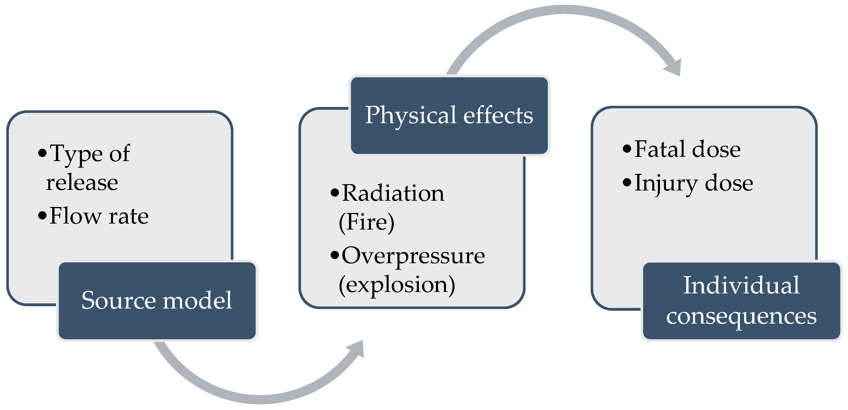
2.2.3. Consequence Analysis

The consequence analysis can be divided into three stages as represented in Figure 2.

The first stage corresponds to the estimation of the release flow rate, which depends on the failure size. For liquid leakage scenarios, a simple model has been proposed for hydrocarbon pipelines and is represented by [27].

$$\dot{m}=0.68D_e^2\sqrt{\rho P_1}$$

(3)

where $\dot{m}$ is the mass flow of the release in kg/s, $\rho$ is fluid density in kg/m³, $P_1$ is the pressure inside the pipe in Pa, and $D_e$ is the equivalent diameter of release in m. This equation is suitable for liquid leakages from pipelines with discharge coefficient of 0.60.

This flow rate is useful to calculate the probability of ignition based on the approach reported by IOGP [28] and given by

$$P_{ignicion}=\{\begin{array}{c}0.00725\ast {\dot{m}}^{0.605},if0.1<\dot{m}<0.3\left(kg/s\right)\\ 0.00408\ast {\dot{m}}^{0.127},if0.1<\dot{m}<70.3\left(kg/s\right)\\ 0.007,if\dot{m}>70.3\left(kg/s\right)\end{array}$$

(4)

The second stage seeks to determine the physical effects associated with the heat radiation and overpressure generated by fires and explosions, respectively. The modeling of fires has been intensely promoted to estimate the physical influence from gas pipeline releases [10,24]. However, modeling fires in oil (or other products) pipelines involves a more complex mix of fluids than gas because of the high number of components. Models developed for oil pipelines include jet fires [28] and pool fires [29].

In the case of jet fires, the heat generated from the single source can be estimated based on the atmospheric transmissivity $\tau$, which may depend on climatological parameters such as precipitation, temperature, cloud cover, or aridity [30]; a view factor $F$ that relates the receiver with the flame shape (usually cylindrical); the distance from the source $r$; and the heat released by combustion $Q$ by unit time. There are different approaches that can be implemented in this regard classified as a point source, multiple point source, or surface emitter models [31,32]. However, a simplified model can be implemented through Equation (5), which has been implemented recently by Cunha [29] to estimate the jet fire heat flow $q^{″}$:

$$q^{″}=\frac{FQ\tau }{4\pi r^2}$$

(5)

where $Q$ is determined by the fluid heat of combustion $\mathsf{\Delta }{H}_c$ and the mass flow as $Q=\mathsf{\Delta }{H}_c\dot{m}$.

Regarding pool fire modeling, there are different approaches that can also be described from a point source models or emissive power (see Yellow Book [32]). These methods mainly depend on the calculation of the pool diameter, weather parameters (i.e., wind velocity) to form an inclined cylinder flame geometry, and the possibility of soot covering. For instance, from an emissive perspective, the Equation (6) can be considered:

$$q^{″}=SE{P}_{act}F\tau$$

(6)

where $SE{P}_{act}$ is the actual surface emissive power, which is determined from the fraction of the generated heat radiation of flames, the heat of combustion, the pool fire dimensions, and the emissive power of soot covering the flames. Further details of these methods can be found in Mudan [29] and TNO [32]. There are other approaches that also can be used that involve simulation software such as EDF or CFD [33]; however, they usually require significant computational resources that may not be recommended for long onshore oil pipelines risk assessment.

Finally, the third stage concentrates on estimating the physical consequences on people, which is basically related to the probability of fatalities or injuries depending on the received physical effect dose. Therefore, this stage covers a procedure to calculate the thermal dose unit and then the effects on people based on some thermal dose fatality thresholds as proposed by HSE [34]. For this purpose, the physical effects on people can be estimated using a thermal dose unit (tdu) based on the heat radiation $q^{″}$ emitted from the fire in kW/m² and the exposure time in seconds as shown in the Equation (7), where some thresholds from fatality assessments can be implemented as those reported by HSE [34]:

$$tdu=t{q}^{{}^{″}\frac{4}{3}}$$

(7)

2.2.4. Risk Level Estimation

The risk can be estimated using the results of the previous steps. The risk can be expressed by using indicators which usually involve both individual and societal levels. In general terms, the individual risk is the probability of death experienced by a hypothetical individual located around the pipeline from certain hazard scenarios [35]. Some of the most common examples are the individual risk per annum (IRPA) [36] and the location-specific individual risk per annum (LSIR) [37]. On the one hand, IRPA considers the fraction of the year in which an individual is exposed to the risk, and it can divide the population in different groups (e.g., operators, work office, public, etc.).

IRPA can be determined using Equation (8), where ${\theta }_k$ is the overall fraction of time that a hypothetical member of a population group $k$ are located on the area of interest, $p_{loc,i,k}$ is the probability that a member of this group be in a particular location $i$, and $Fo{F}_i$ is the frequency of fatality associated with the individual risk for the hypothetical person who stays in a specific location $i$. The latter frequency depends on the frequency of the final event (e.g., pool or jet fire), the probability that the weather conditions promote this scenario, the probability that the scenario is directed to a given location of interest, and the probability of a fatality given the physical dose.

$$IRP{A}_k={\theta }_k{\displaystyle \sum }_i{p}_{loc,i,k}Fo{F}_i$$

(8)

On the other hand, the societal risk is the relationship between the frequency of an accident and the number of people exposed to the hazard scenario that can die as a direct result [38]. The most common representation of societal risk is the F–N diagram in which is possible to differentiate between events with high frequency and involving a low number of fatalities, from those with low frequency and resulting in high number of fatalities. Based on this, the expected fatalities in each location, for a specific final event can be described using the number of individuals in the desired location and the fatality frequency from the physical effect. Note that this number of people depends on the time of the day (i.e., morning, afternoon, night), and the conditions already described for the IRPA index.

The choice between the different indicators of individual or social risk will depend on the criteria against which it will later be compared. In some countries, the criteria are already established by local regulations, while in others companies can use good practice criteria.

3. Results

The methodology is applied to a case-study for illustrative purposes. The case study consists of a segment of a crude oil pipeline located in the southwest region of Colombia. This system is of interest because it is frequently subject to third-party actions and illegal tapping. Moreover, the time of operation of this pipeline also represents a major concern because it has been in service for more than 50 years and the failure rates due to wear-out and corrosion are significant. The pipeline transports 13,514 m³ of liquid hydrocarbons per day. Along the pipeline, the diameter ranges from 0.2540 to 0.4572 m and there are three pumping stations, four pressure reduction stations, and 23 blocking valves.

3.1. System Definition

The case study corresponds to a pipeline segment with a total length of 17.53 km. The pipeline diameter and wall thickness are 0.3556 and 0.0071 m, respectively. The pipeline is laid underground and the cover depth ranges from 1.7 to 1.9 m. The operating flow rate under normal conditions is 564.4 m³/h. The crude oil is transported at 3.7 MPa and a temperature of 30 °C. The segment is located between a pressure reduction station (at 231.49 km from the starting point) and a blocking valve (at 249.02 km). The valves are operated remotely and the maximum closure time for each valve is 10 min. The total crude oil volume in the segment is 1741 m³.

The route of the pipeline goes through two populated locations within a rainforest area where the elevation is approximately 206 m above sea level. The annual average relative humidity is 85% and the annual average wind velocity is 3.5 m/s. The transported liquid is a crude oil of 880 kg/m³ (29.3 API) and a dynamic viscosity is 0.02 Pa s. The crude oil is flammable, as well as the generated vapors. The lower and upper flammability limits are 0.9 and 7.0 (% v/v), respectively. The flash point is −6 °C and the auto ignition temperature ranges from 10 to 20 °C. The relative density of the vapor ranges between 3 and 5 times the density of air.

3.2. Risk Assessment

3.2.1. Hazard Identification

The failure scenarios considered for this study include leakages and rupture of the pipeline. The leakage scenarios considered three holes size: 0.0020, 0.0250, and 0.0500 m. A rupture scenario which can lead to either a pool fire or a spill was also considered. The possibility of a jet fire occurrence is discarded because the liquid tends to fall on the ground quickly and form a pool [25]. It was assumed that this release is caused by a full-bore rupture with a failure size of 0.3556 m. All hazard scenarios to be analyzed with their respective outcomes are summarized in

Table 2. Hazard scenarios considered for the case study.

Hole Diameter (m)	% Sectional Area of Pipe	Outcomes
0.0020	0.56	Jet Fire
		Pool Fire
0.0200	7.03	Jet Fire
		Pool Fire
0.0500	14.06	Jet Fire
		Pool Fire
0.3556	100.00	Pool Fire

.

3.2.2. Frequency Analysis

The frequency analysis requires historical data related to pipeline failures. In Colombia, operators must report every spill incident to the local environmental authority ANLA. This report contains information related mainly to the cause of the release, if fires and explosions were generated, and which components of the environment were affected. However, the reports do not state the failure size, representing a drawback for performing the analysis. Between 2017 and 2020, 31 releases from the pipeline were reported. The failure rate was determined from this data with a result of 2.54 × 10⁻² km⁻¹ yr⁻¹.

Regarding the hole size frequency, the CONCAWE database [7] was contemplated as it only uses hydrocarbon liquids and presents a wide record of incidents that happened between 1971–2018. For the case study, the failure rate had to be adjusted according to length of segment and the frequency of each failure size. For this purpose, the failure sizes of 0.0020, 0.0250, 0.050, and 0.3556 m were considered as pinholes, fissure, hole, and rupture, respectively.

The failure rate in the segment was calculated by multiplying the overall failure rate by the segment length resulting in a value of 4.45 × 10⁻¹ yr⁻¹. Then, the failure frequency by hole size was estimated, obtaining the results shown in

Table 3. Failure frequency (yr⁻¹) for each failure size scenario.

Hole Diameter (m)	Frequency (%)	Failure Frequency (yr−1)
0.0020	11.75	5.23 × 10−2
0.0250	53.92	2.40 × 10−1
0.0500	15.96	7.11 × 10−2
0.3556	18.37	8.18 × 10−2

.

3.2.3. Consequences Analysis

For the case study, the flow rate of the release was calculated considering the model presented by Aloqaily in [27] (Equation (3)) with the following assumptions:

• The flow rate of release is constant. This was only considered for the period where valves are not completely closed.
• The variation in altitude between the start and end points of the pipeline segment was not considered.
• The flow rate for the rupture scenario is equal to the pumping rate.

The results of flow rate for each failure scenario are an input to estimate the probability of ignition following the model presented in the Equation (4). The result corresponds to the sum of immediate and delayed ignition. The probability of immediate ignition is assumed to be 0.001 and this value is taken for all jet fire scenarios. For the pool fire scenarios, the delayed probability value was considered.

Table 4. Release flow rate (kg/s) and probability of delayed ignition for each failure size scenario.

Hole Diameter (m)	Release Flow Rate (kg/s)	Probability of Delayed Ignition
0.0020	0.18	0.0013
0.0250	28.19	0.0051
0.0500	97.00	0.0060
0.3556	137.96	0.0060

shows the flow rate and the probability of delayed ignition for each scenario of pipeline failure.

The analysis of consequences for the jet fire scenarios was carried out using the model for liquid pipelines described by Aloqaily [27] and presented in the Equation (5). For the case study, the following assumptions were considered:

• Release flows in a vertical direction;
• The crater formation was not considered;
• As the pipeline segment is buried, the jet fire was modeled occurring at ground level [23];
• The factor view and atmospheric transmission were 0.3 and 1.0, respectively.

The density and heat of combustion of the crude oil are 880 kg/m³ and 45,107.86 kJ/kg, respectively [39]. For each scenario, the distance where the heat radiation is 37.5 kW/m² was calculated. This radiation value represents a criterion that causes an immediate fatality to the personnel [34]. The results are shown in

Table 5. Distance at the heat radiation is 37.5 kW/m² for each failure scenario.

Hole Diameter (m)	Distance (m)
0.0020	2.1
0.0250	26.4
0.0500	52.5

.

The scenarios involving pool fires were analyzed by using the model presented in Equation (6) based on the reports of Mudan [29] and TNO [32]. For the case study, it was considered that:

• The pool formation occurs at ground level and crater formation was not present;
• The flames generated were modeled as inclined cylinders;
• The fraction of flames covered by soot is 80% [40];
• The fraction of generated heat radiation from flames is 20%;
• The annual average value of wind speed and relative humidity in the location of the case study are 3.5 m/s and 85%, respectively;
• The diameter of the pool was calculated with the expression developed by Aloqaily [27] given by $D=135\sqrt{v}$, where $v$ is the volumetric flow rate of the release in m³/s.

For the case study, the heat radiation of 37.5 kW/m² was also used as criteria to calculate the distance where an immediate fatality could take place [34].

Table 6. Pool diameter and distance at 37.5 kW/m² for each failure size scenario.

Hole Diameter (m)	Pool Diameter (m)	Distance (m)
0.0020	1.79	1.2
0.0250	22.41	12.9
0.0500	44.82	25.7
0.3556	53.45	30.5

shows that distance and the pool diameter for each failure scenario.

The results of Table 4 and Table 5 show that the distance at which a radiation of 37.5 kW/m² is generated in jet fires is approximately twice compared to that in pool fires. In other words, the heat radiation flux generated in jet fires is greater than in pool fires for the same failure scenario. This situation is partly related to the simplicity of the jet fires model by not considering the formation of soot, which may result in an overestimation of the radiation that is generated.

The thermal dose unit (tdu) for all scenarios was calculated using the Equation (7) and the procedure described by HSE [34], considering a time exposure of 20 s [13]. The criteria for determining the effects of thermal radiation on people are shown in

Table 7. Thermal dose fatality criteria. Calculations made based on data selected and extracted from [34].

Thermal Dose Unit (kW/m2)4/3s	Effect
1000	1% Fatality
1800	50% Fatality

.

The goal is to calculate the distance where a person is exposed to these values of thermal radiation and determine the probability of death.

Table 8. Exposure distances to 1800 and 1000 tdu.

Hole Diameter (m)	Outcomes	Distance at 1800 tdu (m)	Distance at 1000 tdu (m)
0.0020	Jet Fire	2.3	3.0
	Pool Fire	1.5	2.1
0.0200	Jet Fire	29.0	37.2
	Pool Fire	16.5	20.6
0.0500	Jet Fire	57.6	74.2
	Pool Fire	31.6	38.0
0.3556	Pool Fire	37.4	45.0

shows the distances where the thermal doses of 1800 and 1000 tdu are generated.

The results of Table 8 show that in scenarios where the failure size is 0.0020 m, the exposure distances (1800 and 1000 tdu) are not significantly different and the effects of thermal radiation are only extended for a few meters. This means that only those workers that are in the immediate vicinity of the pipeline at the time of exposure would be affected. For those scenarios where the failure size is 0.0200, 0.0500 y 0.3556 m, the exposure distances at a thermal dose of 1800 tdu are actually larger than the right-of-the-way of the pipeline (15 m). This means that thermal radiation effects could affect workers as well as people living around the vicinity of the pipeline. This is an important remark because it is not uncommon to find this situation in developing countries such as Colombia. People tend to live in these areas, which means that in terms of time, the risk of exposure is higher compared to workers. As previously described, it can also be seen that in jet fire scenarios the effects of thermal radiation are more far-reaching than in pool fires.

3.2.4. Risk Analysis

The individual and societal risk indicators were estimated considering operation, maintenance, and administrative workers, and people living near to the pipeline as the population groups of interest. The following assumptions were made:

• The operation and maintenance personnel are 20 persons who work 12 h shifts for 15 days per month. This yields an overall fraction of the years spent of 0.25;
• The administrative personnel are 6 persons who work 8 h shifts for 5 days per week. The overall fraction of the year spent is 0.23;
• The probability of being in the right of way of the pipeline is 100% for operation and maintenance personnel and 15% for administrative personnel;
• The populated locations that are close to the segment of the pipeline (denoted as A and B) have 3198 and 1445 inhabitants, respectively;
• The average distance between the pipeline and populated locations A and B, are 23 m and 28 m, respectively.

The individual risk per annum for the population groups of interest was calculated in two steps. First, the individual risks for a hypothetical person standing in a specific location. This value is then converted to the individual risk for a hypothetical member of a specific population group, considering the probability that the hypothetical member of the population group is at the specific location and the overall fraction of time spent there.

As the work conditions for both operation and maintenance of the pipeline are similar, these workers were considered to be within the same population group. The probability of weather conditions required for producing a given scenario is assumed to be 100%. The events in each scenario are considered omni-directional, which means that the probability of each scenario being directed to any direction within the right of way of the pipeline is 100%.

The results of individual risk per annum (IRPA) expressed in yr⁻¹ for operation and maintenance workers (OMW), and administrative workers (AW) are shown in

Table 9. Individual risk per annum for operation and maintenance, and administrative workers.

Hole Diameter (m)	Outcomes	IRPA for OMW (yr−1)	IRPA for OMW (yr−1)
0.0200	Jet Fire	6.00 × 10−5	8.34 × 10−6
	Pool Fire	1.78 × 10−5	2.47 × 10−6
0.0500	Jet Fire	3.07 × 10−4	4.26 × 10−5
	Pool Fire	1.07 × 10−4	1.48 × 10−5
0.3556	Pool Fire	1.07 × 10−4	1.70 × 10−5
	Total	6.14 × 10−4	8.52 × 10−5

. The scenarios using a failure size of 0.0020 m were not included because the IRPA is nearly zero and, therefore, they are not representative in the sum of the total IRPA.

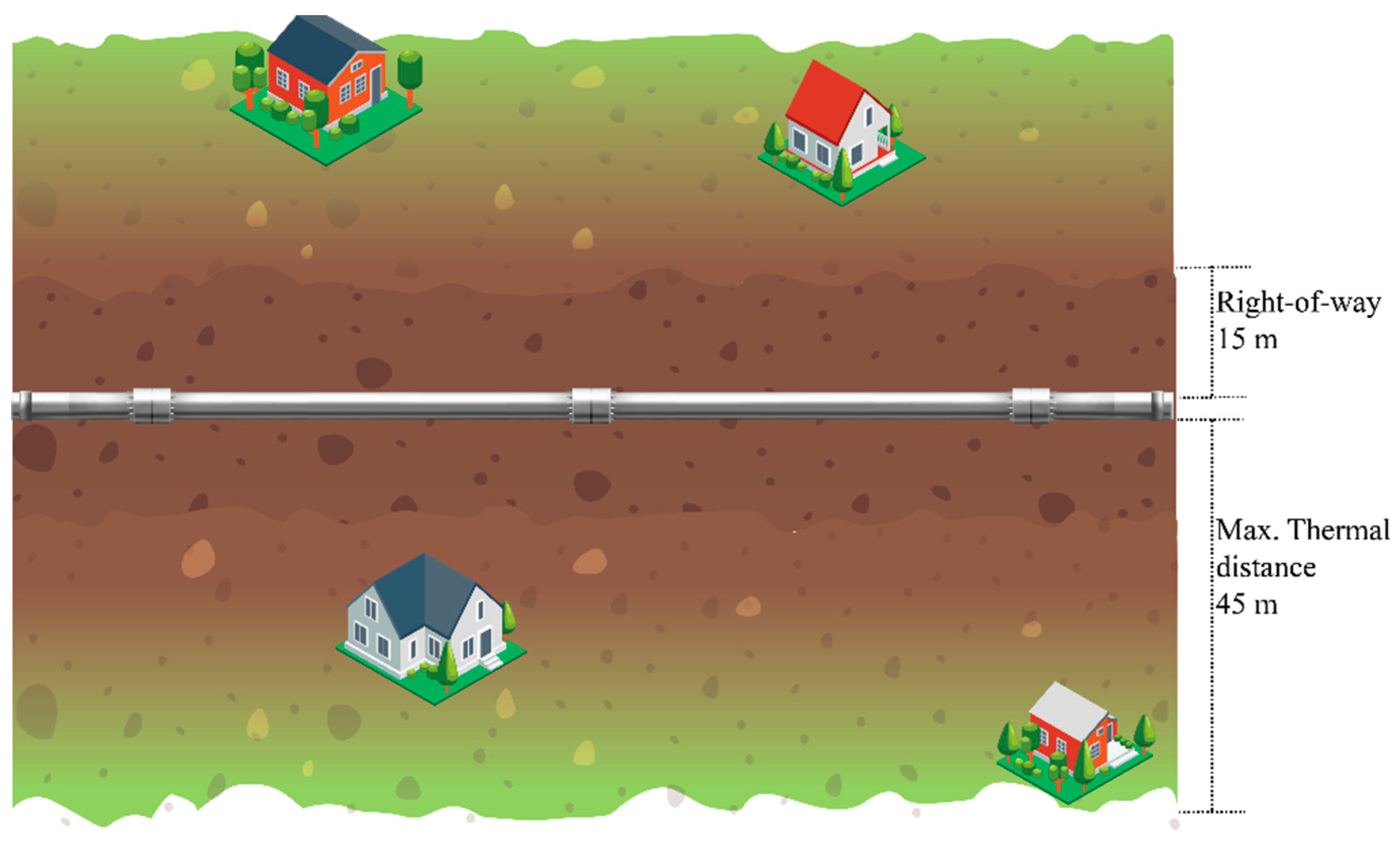
The calculation of the IRPA for the people living within the vicinity of the pipeline was carried out for two segments that pass through populated areas. For this purpose, it was assumed that the population density was uniform along the route of the considered segments. Moreover, the analysis assumed that people are located in a strip from the end of the right of way to the maximum distance where thermal effects could affect the population, as illustrated in Figure 3.

The results of the individual risk per annum for people living in locations A and B are shown in

Table 10. Individual risk per annum for people in the locations A and B.

Hole Diameter (m)	Outcomes	IRPA for People in Location A (yr−1)	IRPA for People in Location B (yr−1)
0.0200	Jet Fire	2.79 × 10−5	2.48 × 10−5
	Pool Fire	2.85 × 10−6	2.53 × 10−6
0.0500	Jet Fire	1.65 × 10−5	1.47 × 10−5
	Pool Fire	9.89 × 10−5	8.79 × 10−5
0.3556	Pool Fire	1.14 × 10−4	1.01 × 10−4
	Total	2.60 × 10−4	2.31 × 10−4

.

The results in Table 9 show that the scenarios where failure size of 0.0500 m and jet fire occur, contributes to more than 50% to the total IRPA. However, the IRPA for OMW is approximately an order of magnitude higher than that for AW. This highlights the importance of considering the annual exposure time of each population group to the hazard scenarios. On the other hand, the results from Table 10 show that the IRPA for people is higher than that for AW, due to house residents being present almost all the time at the vicinity of the pipeline. Nonetheless, the IRPA for people is lower than that of OMW, even though the exposure times are similar. This is because OMW are closer to the pipeline and therefore, the effects of the thermal radiation generated are potentially more harmful.

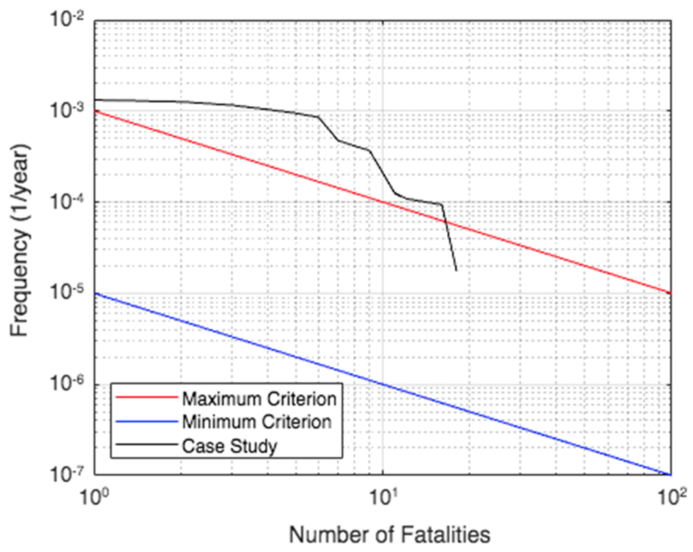
The societal risk was calculated for the same population groups as in the individual risk calculation. However, it was considered that during the daytime 16 people work in operation and maintenance and 6 people work in administrative tasks, while only 6 people work in operations and maintenance at night. The results are plotted in an F–N curve where the x-axis is the expected number of fatalities and the y-axis is the cumulative frequency. Moreover, the maximum and minimum criterion lines were plotted, as shown in Figure 4. For an accident with certain number of expected fatalities, for example 10, the minimum and maximum criteria are 10⁻⁶ yr⁻¹ and 10⁻⁴ yr⁻¹, respectively. This means that if the case study curve lies below 10⁻⁶ yr⁻¹, the societal risk is acceptable; between 10⁻⁶ yr⁻¹ and 10⁻⁴ yr⁻¹, the societal risk is tolerable and finally, above 10⁻⁴ yr⁻¹, the societal risk is unacceptable.

4. Discussion

The individual and societal risk indicators need to be compared to established criteria to determine if risk is acceptable, tolerable, or unacceptable. Although the National Disaster Risk Management System of Colombia (UNGRD) recently published the maximum individual risk level (Resolution 0559 of 2022), both the individual and societal risk criteria of the UK [36] were implemented for illustrative purposes of this work.

The individual risk indicators for workers were compared to the UK acceptability criteria which establish a maximum and minimum criterion of 10⁻³ and 10⁻⁶ per year, respectively. The individual risk per annum for OMW is within the ALARP region which means it is tolerable. However, considering its proximity to the maximum criterion, it requires implementing some risk reduction measures based on the results of a cost–benefit tradeoff analysis. Regarding the individual risk for AW, note the results are relatively higher than the broadly acceptable criterion, so it seems that no further measures are required. Furthermore, the maximum and minimum criteria in the UK [36] for people in the vicinity of the pipeline are 10⁻⁴ and 10⁻⁶ per year, respectively. The individual risk per annum for people in both segments considered is unacceptable because it is higher than the maximum criterion. This means that the implementation of measures to reduce the risk to tolerable or acceptable levels is mandatory, regardless of their costs. Nevertheless, the first step could be to perform a deeper analysis of the consequences considering more complex models to recalculate the individual risk per annum.

Figure 4 shows the F–N curve for the case study and the acceptability criteria for societal risk established in the United Kingdom. The curve is above the maximum criterion almost all the time, which means that the societal risk for the case study is unacceptable. This result may indicate that the operation requires reducing the risk to tolerable or acceptable levels. The behavior of the curve may be related with the uncontrolled increase in the residents in both evaluated locations. Thus, the operator and local planning departments could contemplate relocating nearby people exposed to the pipeline risk operation to safer areas. Additionally, the operator is recommended to incorporate further risk treatment measures, especially those focused on reducing the frequency of those hazard scenarios.

5. Conclusions

A quantitative risk assessment approach is described for oil onshore pipelines. The approach contemplated a frequency-based result with the evaluation of fire scenarios (i.e., jet and pool fire) with a thermal dose response in individuals. This approach seeks to support decisions from a risk perspective using individual and societal risk indicators, which in turn, can help set the basis for further risk evaluation and risk treatment. An application of the approach was carried out on a 17.53 km length segment of an oil pipeline located in the southwest of Colombia. A total of seven scenarios resulting in jet fires and pool fires were considered.

The results show that individual risk was 6.14 × 10⁻⁴ yr⁻¹ for operation and maintenance workers and 8.52 × 10⁻⁵ yr⁻¹ for administrative workers. These values are in the ALARP region which means the risk is tolerable. The pool fire resulting from a failure of 0.050 m was the scenario which contributed the most to the individual risk, representing approximately 50%. The individual risk for people calculated for the segments passing through two nearby locations were 2.60 × 10⁻⁴ and 2.31 × 10⁻⁴ yr⁻¹, respectively. These values are above the maximum acceptability criteria which means the risk is unacceptable and risk reduction measures must be considered to continue with the pipeline operation. On the other hand, the societal risk was assessed using a F–N curve, having results surpassing the maximum criterion. This situation requires implementing measures for reducing the risk, especially of these scenarios which contribute the most to the risk level.

The results of the methodology cou”d yi’ld more reliable values by using representative information of the operation of oil pipelines in Colombia, such as frequency of size failures. Furthermore, the establishment of a risk maximum criterion (Resolution 0559 of 2022) will allow comparing further risk assessments results under the environmental licensing processes of oil pipeline projects.

This work proposes an approach that aims to be a QRA screening result of an oil pipeline based on individual and societal indicators. This approach does not require specialized software and can be seen as a preliminary assessment for deeper risk analyses.