Abstract
This article’s goal was to explain how chemical reaction and viscous dissipation affect a
non-Newtonian Cross-fluid in a boundary layer flow due to a stretching sheet with variable fluid
properties. The results were obtained after assuming laminar, steady, and viscous flow characteristics.
In this study, the analysis took into account the characteristics of the fluid variable diffusivity
and slip velocity. It was considered that fluid viscosity and thermal conductivity are temperaturedependent
variables. Because of their mobility, non-Newtonian fluid particles are thought to interact
chemically. The physical problem is governed by a set of partial differential equations that are not
linear. Anumerical solution was reached usingNewton’s shooting methodology and the Runge–Kutta
integration technique. A set of figures displays the distributions of the temperature, concentration,
and velocity at various physical parameter values. The influence of all physical parameters is shown
in tabular form together with the local Sherwood number, drag force, and local Nusselt number. A
key conclusion was that the temperature profile of the nanofluid increases as the mixed convection
parameter and Eckert number rise. Furthermore, both the Sherwood number and the Nusselt number
decreased as the slip velocity parameter increased. Last but not least, the results proved that the
suggested numerical approach, which offers a reliable description of the flow and heat mass transfer
mechanism, is effective.
1. Introduction
For scientists, the study of non-Newtonian fluid flow has theoretical, as well as practical applications. These fluids are used in a variety of products in both the natural and industrial worlds, such as drilling mud, pulps, oils, poly crystal melts, certain paints, fluid suspensions, emulsions, cosmetic and food items, and more. The Newtonian theory is challenged by the non-Newtonian fluids’ behavior. Non-Newtonian fluid models, such as the power-law fluid model [1], have been proposed by multiple researchers due to the non-Newtonian fluids’ enormous practical utility. In numerous actual problems, the power-law representation of the non-Newtonian materials has been verified. Simply adding the power-law model as an extra phrase to represent the Newtonian behavior at low shear rates can explain some fluid types that depart from their characteristics. It seems that Matsuhisa and Bird [2] came up with this concept first. Since then, numerous scientists and engineers have addressed various non-Newtonian problems numerically and analytically in a variety of physical situations; some of them fall within the category of viscoelastic models [3,4], and others fall within the power-law category [5,6,7,8]. The flow primarily follows the power-law concept in all of these previous studies. The phenomenon of slip velocity, which is crucial in the flow of viscous fluids [9], is the subject of our investigation. The thin layer of the fluid flowing streamwise due to a rough sheet just inside the boundary layer is essentially, which causes the slip velocity phenomenon. Additionally, taking into account the slip phenomenon helps to describe a few problems in a variety of additional applications [10].
The findings stated above are only applicable to a few physical phenomena in the non-Newtonian power-law model. The non-Newtonian power-law type has numerous and significant application possibilities, although it is still lacking in many areas, particularly when shear rates are extremely low or extremely high. At the same time, it is unable to provide a thorough description of the fluid behavior in these delicate situations. As a result, the Ellis model [11] is used to address cases that the power-law model is unable to express. Generalized Newtonian fluids are a class of models that the Ellis model belongs to [12]. The Ellis model is demonstrated through a series of experimental investigations to be a very advantageous empirical technique for engineering disciplines, whether for analytical and numerical solutions or for dimensional analysis needs. To overcome all prior constraints, in particular those related to extremely low and extremely high shear rates, the cornerstone of a novel rheological model was first given by pioneering researcher Cross [13]. Because the Cross model has a time constant, it is extensively employed in engineering analysis. The synthesis of polymeric solutions, blood, aqueous Xanthan gum solution, and aqueous polymer latex sphere solution are a few examples of the uses of the Cross model [14]. Some current boundary layer flow problems regarding non-Newtonian Cross fluid were further researched while taking the potential applications into account for a viscous Cross fluid by Xie and Jin [15], by Khan et al. [16] for Cross fluid due to a stretching sheet, by the same authors Khan et al. [17] due to a radially stretching sheet, by Khan et al. [18] for the magnetohydrodynamic stagnation point flow of Cross fluid, by Manzur et al. [19] under the impact of thermal radiation on the flow characteristics of a non-Newtonian Cross fluid, and by Mustafa et al. [20] under the influence of Arrhenius activation energy and binary chemical reaction.
The innovative aspect of the current work is the investigation of the relationship between the phenomenon of slip velocity and variable fluid properties in a reactive non-Newtonian Cross fluid. This study is ground breaking since it is the first to evaluate how a stretched vertical sheet affects the flow and heat mass transfer of the Cross model. Through this study, considerations were made about viscous dissipation. With the use of the shooting technique, the model equations were numerically solved, and graphs were used to show how new parameters affect the fluid’s velocity, temperature, and concentration. Finally, by comparing the numerical technique proposed here to the literature already in existence for the limiting cases, the numerical method was verified.
2. Problem Formulations
Here, we took into account the steady two-dimensional incompressible flow, heat, and mass transfer of a non-Newtonian Cross fluid with viscosity toward a vertically stretched slippery sheet. The design of the current flow problem is illustrated in Figure 1. It was assumed that the surface sheet has a concentration of and a temperature of . Furthermore, regulates how quickly the stretching sheet moves, where a is an index of stretching with unit s. Let stand for the fluid’s ambient temperature and for its concentration. Likewise, the Cross fluid is characterized by the index m, which measures how fluid viscosity is influenced by the shear rate. In light of the existence of the viscous dissipation phenomenon, frictional heating was looked into. The remaining fluid properties were taken to be constant, with the exception of the fact that the study considered the impact of both thermal conductivity and the fluid’s variation in viscosity with temperature.
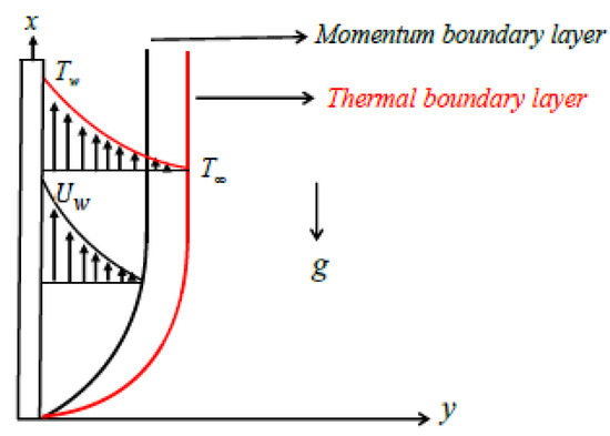
Figure 1.
Schematic diagram.
The fundamental equations for a Cross fluid that account for the presence of viscous dissipation in the energy equation and the chemical reaction mechanism in the concentration equation [21,22,23,24] can be expressed as follows using the standard boundary layer approximations [25]:
where, along with the x- and y-directions, u and v represent the components of the velocity, respectively. is the ambient fluid density; is the coefficient of thermal expansion; is the Cross time constant; g is the gravitational acceleration. Further, T is the fluid’s temperature; the amount of specific heat at a given pressure is ; D is the fluid variable diffusivity; is the fluid thermal conductivity; K is the chemical reaction rate. The conditions that govern the stretching operation are now described by mathematical formulas. The following conditions outline the thermal mechanism and the concentration situations, as well as the sheet’s impervious state:
Here, is a factor affecting slip phenomenon, and is the ambient fluid viscosity. Further, as a succinct explanation of the conditions and presumptions used in Equation (5), the first portion describes the slip velocity phenomenon, while the second portion means that the sheet is impermeable, whereas the third and fourth parts represent the fluid temperature and the fluid concentration, respectively. The following non-dimensional quantities are introduced [25]:
where f is the non-dimensional stream function, is the similarity variable, is the dimensionless temperature of the fluid, and is the dimensionless fluid concentration. Additionally, the following relations can be used to control the relationship between the stream function and the velocity components:
The momentum equation and the energy equation depend on the precise structure of the fluid viscosity and the fluid thermal conductivity , which several researchers have previously extensively introduced, because they are temperature-dependent. Following Mahmoud and Megahed’s work [26], we have:
Here, is a factor affecting the viscosity, is the constant thermal conductivity at the ambient temperature, and is a parameter controlling the fluid conductivity. The diffusion coefficient D, which Mohyud Din et al. [27] discovered earlier, may also be modeled as a function of the concentration when the parallels between heat and mass transport are taken into account as:
where is the ambient diffusivity and is the variable diffusion parameter. When the aforementioned Equation (9) is inserted into the continuity Equation (1), the continuity equation is immediately achieved. Additionally, by replacing the dimensionless variable Equations (7)–(9) in the momentum Equation (2), the energy Equation (3), and the concentration Equation (4), we are able to construct the governing ordinary differential equations with boundary conditions, which are written in terms of the dimensionless velocity , dimensionless temperature , and dimensionless concentration as follows:
where is the local mixed convection parameter, is the local Eckert number, is the local Weissenberg number, is the slip parameter, is the Prandtl number, and is the chemical reaction parameter. Here, we must mention that (), (), and () are the local parameters since they depend on the length scale (x). It is crucial to keep in mind that the provided governing equations only hold true for a locally similar solution [28] because these parameters are functions of x, and their changes take place locally during the flow activity. As a result, we provided exact values for , , and for the current graphical results, which apply to the flow study for a certain value of x and for all values of y. Following immediately, the standard definitions of the shear stress at the wall , the Nusselt number , and the local Sherwood number are as follows:
where is the local Reynolds number.
3. Numerical Methodology
Following the use of the shooting approach to determine the fluid velocity, concentration, and temperature changes for the transient response of the system, the governing equations describing our problem have been numerically solved. Compared to other numerical approaches, the shooting strategy is more flexible because the convergence conditions are predetermined by the initial guesses. Equations (12)–(14), together with the boundary conditions (15)–(16), are linked highly non-linear ordinary differential equations. Consequently, we used the numerical shooting method coupled with the Runge–Kutta integration approach. Here, the regulating boundary value problem was simplified to a system of seven concurrently coupled first-order ordinary differential equations. Therefore, we firstly assumed that
Equations (12) through (14) were then simplified to a system of first-order ordinary differential equations, i.e.,
where , and were chosen so that the outer boundary criteria , and are met. The choice of the suitable value at infinity () is one of the crucial components of this strategy. Until the outer boundary conditions are fulfilled, the shooting method is employed to iteratively guess the values for , and . After that, the Runge–Kutta fourth-order integration strategy can be used to integrate the resulting differential equations. Up until the results reach the necessary level of precision , the aforementioned process is repeated.
4. Shooting Technique Verification
The shooting approach was used to provide numerical solutions to the physical boundary value problem proposed here. In light of the research problem, one suitable numerical solution is the numerical shooting method used in the present study. The shooting method provides the advantage of using procedures for initial value problems that are quick and flexible. Our problem was evaluated for different slip velocity values if the mixed convection, the viscosity, and the local Weissenberg parameters are not present (). The findings are summarized in Table 1. In limiting cases, we examined the results of , obtained with those of Andersson [29]. This offered us assurance that our findings are reliable and more comprehensive than those of earlier investigations.

Table 1.
Values of with different values of .
5. Discussion of the Results
Particular attention was paid to how physical parameters affect heat mass transfer with magnetic fields and thermal radiation, as well as fluid flow due to a stratified stretched sheet in the thermal area. The system that controls the problem was resolved using the shooting approach. Figure 2a,b are plotted to show how the flow behavior index m affects both fluid flow and mass heat transfer. Regarding various values of the parameter m, the function is plotted vs. the parameter in Figure 2a. Clearly, as , the rate of the flow changes towards it, achieving greater values with a higher m. In contrast, the heat and mass flow rate show an inverse tendency. As m rises, this behavior develops as a result of the increasing momentum barrier layer. The axial contraction of the boundary layer, which results in a thickening of the boundary layer in the transverse direction, is the physical explanation for the increase in the boundary layer thickness. Finally, it is important to note that the behavior of the parameter m on both the velocity and the temperature distribution is identical to that of Khan et al.’s [17] earlier work.
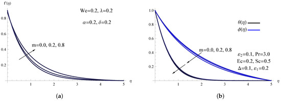
Figure 2.
(a) for assorted m; (b) and for assorted m.
Figure 3a,b are plotted for different values of the parameter . These figures show the effects of on the fluid flow rate and heat mass transfer. As can be observed, the fluid velocity becomes noticeable if the local Weissenberg number is low enough. Additionally, as the local Weissenberg number rises, the thickness of the momentum boundary layer reduces. Further, the reverse is observed for the same parameter on the heat and mass flow. It’ is also worth noting that, when increases, the thermal boundary layer becomes thicker. Physically, an improvement in produces an increase in the Cross time constant , which leads the fluid’s velocity to decrease and the fluid’s concentration, as well as its temperature to rise. Recalling the work of Khan et al. [17] confirms the validity of the behavior of on both the temperature and the velocity distribution.
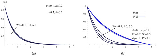
Figure 3.
(a) for assorted ; (b) and for assorted .
The results of the velocity distribution and the temperature distribution for the slip velocity parameter , which runs in the laminar Cross fluid flow region, are plotted in Figure 4a,b. In these figures, the results show that, as increases, the velocity field, the fluid velocity along the sheet , and the boundary layer thickness reduce. Simultaneously, Figure 4b shows that increasing the slip velocity parameter improves both and for the distributions. Physically, the occurrence of the slip velocity parameter creates an obstructing force that causes the Cross-fluid flow to slow down. It is crucial to remember that the action of the slip velocity parameter on the fluid flow characteristics is the same as that of the earlier study of Adem and Kishan [30].
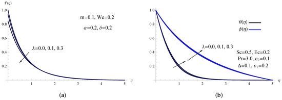
Figure 4.
(a) for assorted ; (b) and for assorted .
Figure 5 shows the impact of the mixed convection parameter on the flow of Cross fluid while keeping all other physical parameters constant. It is important to point out that, when increases, the fluid velocity decreases throughout the boundary layer region. As shown in Figure 5b, the concentration the the temperature fields increases successively by enhancing the values of the mixed convection parameter . The temperature difference between the sheet and the ambient environment is what constitutes the mixed convection parameter physically. Therefore, a high sheet temperature results in the temperature field within the layer of the thermal boundary to accelerate, with the maximum value for the mixed convection parameter.
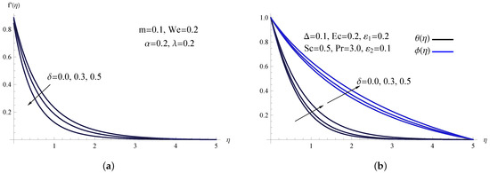
Figure 5.
(a) for assorted ; (b) and for assorted .
Figure 6 expresses the influence of the viscosity parameter on the distribution of the velocity , the fluid concentration , and the fluid temperature . Due to the intensification of the viscosity parameter , the velocity distribution, in addition to the boundary layer’s thickness reduce. On the other hand, Figure 6b attempts to explore the behavior of and for various values of . Physically, having a high viscosity parameter value results in the Cross fluid becoming more viscous, which slows the flow of the fluid. Examining this graph reveals that the viscosity parameter results in an improvement for both the fluid concentration, as well as its temperature.
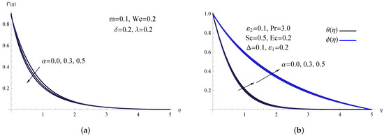
Figure 6.
(a) for assorted ; (b) and for assorted .
In Figure 7a, is sketched versus for distinct values of . As mentioned, the impacts of on are manifested to the maximum extent. The temperature distribution can be seen to increase with . Consequently, the assumption of variable conductivity also decreases the rate of heat transfer at the sheet. It would be interesting to determine the process of cooling, when the sheet has a higher chance of developing, and the maximum value of in a real-world scenario. Figure 7b shows the concentration distribution for various values of the variable diffusion parameter . Likewise, the variable diffusion parameter has a noticeable influence on and the corresponding layer thickness. Additionally, the thermal energy transfer within the thermal boundary region rises as the thermal conductivity parameter elevates, which is the physical cause of the temperature distribution behavior.
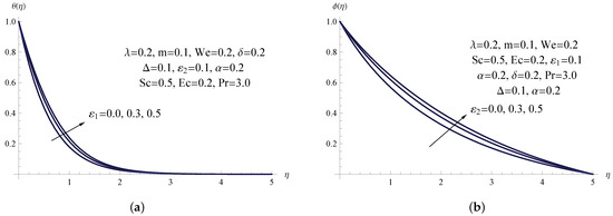
Figure 7.
(a) due to the alteration in ; (b) due to the alteration in .
Figure 8a shows how the Eckert number affects the thermal field . This diagram demonstrates how the Eckert number affects how the temperature curve rises. Figure 8b displays the calculated concentration distribution and the thickness of the solutal layer with the reaction parameter . The thickness of the solutal boundary layer is discovered to decrease with . Additionally, this parameter has a substantial impact on the concentration field due to the increasing significance of this phenomena in the slow mass flow mechanism. Additionally, the results of the Eckert number can be verified by looking back to the earlier work of Rasool et al. [31].
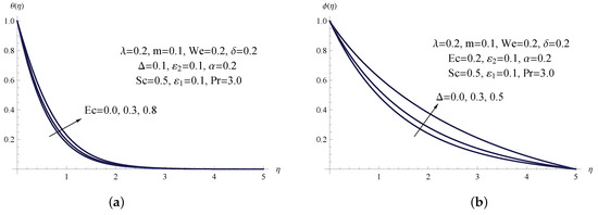
Figure 8.
(a) due to the alteration in ; (b) due to the alteration in .
Finally, Figure 9 shows how the parameter of viscosity affects the mass and heat transport rates in addition to the skin-friction coefficient. This figure demonstrates that, as improves, the local skin-friction coefficient , the Nusselt number , and the local Sherwood number all decrease significantly.
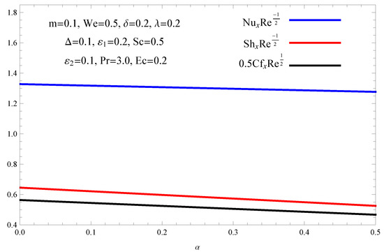
Figure 9.
Effect of on , , and .
Now, the drag force in terms of skin-friction coefficient , the heat transfer rate in relation to local Nusselt number , and the rate of mass transfer according to local Sherwood number , respectively, are shown in the following Table 2 for diverse values of the index parameter m, slip velocity parameter , Weissenberg number , and the parameters , , , , and , with . It was found that the surfaces’ shear stress, the mass transfer rate, and the heat transfer rate decrease as the local Weissenberg number increases. This behavior is due to the thickening of the thermal boundary layers as increases. Further, it was discovered that both the slip velocity parameter and the mixed convection parameter increase the concentration and temperature distributions, while they decrease both the local Nusselt and Sherwood numbers. The same table also depicts that the local Sherwood number is perceived as having a declining function for both variable diffusion and the Eckert parameters. Likewise, it is clear that by improving the values of the local Sherwood number, the chemical reaction parameter improves, whereas the local Nusselt number diminishes.
Table 2.
Values of , , and for distinct values of the governing parameters when and .
6. Conclusions
The current study’s innovative approach was to look into the combined effects of the slip velocity phenomenon and variable fluid characteristics in a reactive non-Newtonian Cross fluid caused by a stretched sheet. Therefore, the study evaluated the computational modeling for the two-dimensional laminar flow of a non-Newtonian Cross fluid with chemical reaction and the slip velocity phenomenon toward a linearly stretched surface. While the fluid thermal conductivity was dependent on temperature, the diffusion coefficient was reliant on concentration. With the assistance of the appropriate transformations, a non-linear system of ordinary differential problems that represent the physical model was obtained. Using the shooting approach, the non-linear systems were calculated. The aforementioned analysis revealed the following crucial facts:
- The local Nusselt number, as well as the coefficient of the local skin-friction are both enhanced by the flow behavior index, whereas the opposite outcome is caused by the slip velocity parameter.
- The thermal conductivity parameter’s presence results in changes to the temperature profile and thermal thickness, in addition to a decrease in the sheet’s rate of heat transmission.
- The research predicted significant changes in the characteristics of heat transfer and fluid flow, in particular for Weissenberg numbers above or around 0.1.
- Due to the existence of the mixed convection phenomenon, the skin-friction coefficient improved, although the local Sherwood and Nusselt numbers showed the opposite trend.
- Increases in the flow behavior index and chemical reaction parameter improved the rate of mass transfer.
Author Contributions
Data curation, H.A.; Formal analysis, M.A.; Funding acquisition, H.A.; Methodology, M.A. All authors have read and agreed to the published version of the manuscript.
Funding
This research received no external funding.
Data Availability Statement
Not applicable.
Conflicts of Interest
The authors declare no conflict of interest.
Nomenclature
| a | velocity coefficient |
| specific heat | |
| C | fluid concentration |
| coefficient of skin-friction | |
| surface fluid concentration | |
| ambient fluid concentration | |
| D | diffusion coefficient |
| ambient diffusivity | |
| Eckert number | |
| f | dimensionless stream function |
| g | gravitational acceleration |
| K | chemical reaction rate |
| m | coefficient of the Cross fluid |
| local Nusselt number | |
| Prandtl number | |
| local Reynolds number | |
| Schmidt number | |
| local Sherwood number | |
| T | fluid temperature |
| ambient temperature | |
| u | velocity component in the x-direction |
| v | velocity component in the y-direction |
| Weissenberg number | |
| Cartesian coordinates | |
| Greek symbols | |
| coefficient of viscosity | |
| ambient fluid viscosity | |
| dimensionless temperature | |
| dimensionless concentration | |
| thermal conductivity of the Cross fluid | |
| ambient Cross fluid thermal conductivity | |
| nanofluid density | |
| ambient fluid density | |
| thermal expansion coefficient | |
| Cross time constant | |
| viscosity parameter | |
| kinematic viscosity | |
| thermal conductivity parameter | |
| variable diffusion parameter | |
| mixed convection parameter | |
| slip velocity parameter | |
| chemical reaction parameter | |
| similarity variable | |
| Superscripts | |
| ′ | differentiation with respect to |
| ∞ | free stream condition |
| w | wall condition |
References
- Acrivos, A.; Shah, M.J.; Peterson, E.E. Momentum and heat transfer in laminar boundary-layer flows of non-Newtonian fluids past external surfaces. AlChE J. 1960, 6, 312–317. [Google Scholar] [CrossRef]
- Matsuhisa, S.; Bird, R.B. Analytical and numerical solutions for laminar flow of the non-Newtonian Ellis fluid. AlChE J. 1965, 11, 588–595. [Google Scholar] [CrossRef]
- Shenoy, A.V. Combined laminar forced and free convection heat transfer to viscoelastic fluids. AlChE J. 1980, 26, 683–686. [Google Scholar] [CrossRef]
- Shenoy, A.V.; Mashelkar, R.A. Thermal convection in non-Newtonian fluids. Adv. Heat Transf. 1982, 15, 143–225. [Google Scholar]
- Vajravelu, K.; Prasad, K.V.; Rao, N.S.P. Diffusion of a chemically reactive species of a power-law fluid past a stretching surface. Comput. Math. Appl. 2011, 62, 93–108. [Google Scholar] [CrossRef]
- Mahmoud, M.A.A. Slip velocity effect on a non-Newtonian power-law fluid over a moving permeable surface with heat generation. Math. Comput. Model. 2011, 54, 1228–1237. [Google Scholar] [CrossRef]
- Lin, Y.H.; Zheng, L.C.; Ma, L.X. Heat transfer characteristics of thin power-law liquid films over horizontal stretching sheet with internal heating and variable thermal coefficient. Appl. Math. Mech. 2016, 37, 1587–1596. [Google Scholar] [CrossRef]
- Zhang, Y.; Zhang, M.; Bai, Y. Unsteady flow and heat transfer of power-law nanofluid thin film over a stretching sheet with variable magnetic field and power-law velocity slip effect. J. Taiwan Inst. Chem. Eng. 2017, 70, 104–110. [Google Scholar] [CrossRef]
- Baranovskii, E.S.; Domnich, A.A. Model of a nonuniformly heated viscous flow through a bounded domain. Differ. Equ. 2020, 56, 304–314. [Google Scholar] [CrossRef]
- Domnich, A.A.; Baranovskii, E.S.; Artemov, M.A. A nonlinear model of the non-isothermal slip flow between two parallel plates. J. Phys. Conf. Ser. 2020, 1479, 012005. [Google Scholar] [CrossRef]
- Gee, R.E.; Lyon, J.B. Nonisothermal flow of viscous non-Newtonian fluids. Ind. Eng. Chem. 1957, 49, 956–960. [Google Scholar] [CrossRef]
- Biery, J.C. Numerical and experimental study of damped oscillating manometers: I. Newtonian fluids. AlChE J. 1963, 9, 606–614. [Google Scholar] [CrossRef]
- Cross, M.M. Rheology of non-Newtonian fluids: A new flow equation for pseudoplastic systems. J. Colloid Sci. 1965, 20, 417–437. [Google Scholar] [CrossRef]
- Barnes, H.A.; Hutton, J.F.; Walters, K. An Introduction to Rheology; Elsevier Science: Amsterdam, The Netherlands, 1989. [Google Scholar]
- Xie, J.; Jin, Y.C. Parameter determination for the Cross rheology equation and its application to modeling non-Newtonian flows using the WC-MPS method. Eng. Appl. Comput. Fluid Mech. 2016, 10, 111–129. [Google Scholar] [CrossRef]
- Khan, M.; Manzoor, M.; Rahman, M. Boundary-layer flow and heat transfer of Cross fluid over a stretching sheet. Therm. Sci. 2019, 23, 307–318. [Google Scholar] [CrossRef]
- Khan, M.; Manzoor, M.; Rahman, M. On axisymmetric flow and heat transfer of Cross fluid over a radially stretching sheet. Results Phys. 2017, 7, 3767–3772. [Google Scholar] [CrossRef]
- Khan, M.I.; Waqas, M.; Hayat, T.; Alsaedi, A. Magnetohydrodynamical numerical simulation of heat transfer in MHD stagnation point flow of Cross fluid model towards a stretched surface. Phys. Chem. Liq. 2017, 7, 1824–1827. [Google Scholar]
- Manzur, M.; Khan, M.; Rahman, M. Mixed convection heat transfer to Cross-fluid with thermal radiation: Effects of buoyancy assisting and opposing flows. Int. J. Mech. Sci. 2018, 138, 515–523. [Google Scholar] [CrossRef]
- Mustafa, M.; Aiman, S.; Rahi, M. Pressure-driven flow of Cross fluid along a stationary plate subject to binary chemical reaction and Arrhenius activation energy. Arab. J. Sci. Eng. 2019, 44, 5647–5655. [Google Scholar] [CrossRef]
- Gowda, R.J.P.; Kumar, R.N.; Jyothi, A.M.; Prasannakumara, B.C.; Sarris, I.E. Impact of binary chemical reaction and activation energy on heat and mass transfer of marangoni driven boundary layer flow of a non-Newtonian nanofluid. Processes 2021, 9, 702. [Google Scholar] [CrossRef]
- Gowda, R.J.P.; Sarris, I.E.; Kumar, R.N.; Kumar, R.; Prasannakumara, B.C. A three-dimensional non-Newtonian magnetic fluid flow induced due to stretching of the flat surface with chemical reaction. J. Heat Transfer. 2022, 144, 113602. [Google Scholar] [CrossRef]
- Shah, S.A.A.; Ahammad, N.A.; Din, E.M.T.E.; Gamaoun, F.; Awan, A.U.; Ali, B. Bio-convection effects on Prandtl hybrid nanofluid flow with chemical reaction and motile microorganism over a stretching sheet. Nanomaterials 2022, 12, 2174. [Google Scholar] [CrossRef] [PubMed]
- Shamshuddin, M.D.; Mebarek-Oudina, F.; Salawu, S.O.; Shafiq, A. Thermophoretic movement transport of reactive Casson nanofluid on riga plate surface with nonlinear thermal radiation and uneven heat sink/source. J. Nanofluids 2022, 11, 833–844. [Google Scholar] [CrossRef]
- Megahed, A.M.; Abbas, W. Non-Newtonian Cross fluid flow through a porous medium with regard to the effect of chemical reaction and thermal stratification phenomenon. Case Stud. Therm. Eng. 2022, 29, 101715. [Google Scholar] [CrossRef]
- Mahmoud, M.A.A.; Megahed, A.M. MHD flow and heat transfer in a non-Newtonian liquid film over an unsteady stretching sheet with variable fluid properties. Can. J. Phys. 2009, 87, 1065–1071. [Google Scholar] [CrossRef]
- Mohyud Din, S.T.; Zubair, T.; Usman, M.; Hamid, M.; Rafiq, M.; Mohsin, S. Investigation of heat and mass transfer under the influence of variable diffusion coefficient and thermal conductivity. Indian J. Phys. 2018, 92, 1109–1117. [Google Scholar] [CrossRef]
- Megahed, A.M. Flow and heat transfer of powell-eyring fluid due to an exponential stretching sheet with heat flux and variable thermal conductivity. Z. Naturforsch. 2015, 70, 163–169. [Google Scholar] [CrossRef]
- Andersson, H.I. Slip flow past a stretching surface. Acta Mech. 2002, 158, 121–125. [Google Scholar] [CrossRef]
- Adem, G.A.; Kishan, N. Slip effects in a flow and heat transfer of a nanofluid over a nonlinearly stretching sheet using optimal homotopy asymptotic method. Int. J. Eng. Manuf. Sci. 2018, 8, 25–46. [Google Scholar]
- Rasool, G.; Shafiq, A.; Chu, Y.M.; Bhutta, M.S.; Ali, A. Optimal homotopic exploration of features of Cattaneo-Christov model in second grade nanofluid flow via darcy-forchheimer medium subject to viscous dissipation and thermal radiation. Comb. Chem. High Throughput Screen. 2022, 25, 2485–2497. [Google Scholar]
Disclaimer/Publisher’s Note: The statements, opinions and data contained in all publications are solely those of the individual author(s) and contributor(s) and not of MDPI and/or the editor(s). MDPI and/or the editor(s) disclaim responsibility for any injury to people or property resulting from any ideas, methods, instructions or products referred to in the content. |
© 2023 by the authors. Licensee MDPI, Basel, Switzerland. This article is an open access article distributed under the terms and conditions of the Creative Commons Attribution (CC BY) license (https://creativecommons.org/licenses/by/4.0/).