A Partial Approximate Least Absolute Deviation-Based Identification Algorithm for a Multivariable Closed-Loop System with Spike Noise

Abstract

Considering the stability and safety of industrial production, the open-loop system cannot meet the requirements of industrial production, so more and more attention has been paid to multivariable closed-loop system identification. This study focuses on the identification of a multivariate closed-loop system with spike noise in which the model order of the feedback channel is lower than that of the forward channel. Combining principal component analysis (PCA), which is used to eliminate the correlation between the data matrix elements, and the derivable approximate least absolute criterion function, partial approximate least absolute deviation (PALAD) for multivariable closed-loop system identification is proposed. By introducing a deterministic function to replace the absolute value in partial approximate least absolute deviation, the non-differentiable problem of the least absolute deviation function can be solved, and the identifiability of the multivariable closed-loop system in the case mentioned above is theoretically verified. Simulation experiments show the validity of the PALAD algorithm. Compared with the partial least squares (PLS) method, PALAD can effectively restrain the spike noise that follows an $S\alpha S$ distribution and shows stronger robustness when white and spike noises exist simultaneously.

1. Introduction

Closed loop control is a control method based on the output feedback of the control object. It corrects the regulator according to norms or standards when there is a deviation between the actual measurement and the set-point. Multivariable closed-loop systems are crucial in industrial processes, such as in model-based closed-loop control in the hydraulic fracturing process [1], closed-loop control in the multi-column solvent gradient purification process [2], etc. For many practical industrial processes, cutting off the feedback loop will cause processes to become out of control and will seriously affect production. Closed-loop system identification methods are generally categorized as direct, indirect, and joint input–output approaches [3]. Previous research has shown that if the order of the controller (feedback channel) is not less than that of the process (forward channel), then the closed loop is identifiable [4]. Gevers et al. theoretically provided necessary and sufficient conditions for the informativity of experiments in open-loop and closed-loop operations, and the same conclusion was obtained [5]. Uematsu et al. proposed using routine operation data without extra excitation signals to identify closed-loop systems [6,7]. Vau et al. improved the closed-loop output error identification algorithm by establishing a predictor based on the generalized orthogonal transfer function, which was suitable for unstable systems or controllers [8]. Shardt and Huang focused on the closed-loop identification condition while considering pole-zero cancellations and confirmed the condition further [9]. Multivariable closed-loop systems can be effectively handled by state space models, decentralized identification, and subsystem identification. Notably, the abovementioned studies were based on a controller order that satisfies identifiable conditions [10,11,12]. However, a multivariable closed-loop system whose controller order is lower than that of the process without interference noise in the feedback channel has not elicited much attention. The real issue lies in the linear correlation existing in the elements of the measured data vector through the feedback in multivariable systems, and this leads to the unidentifiability of the parameters [12]. This situation is inevitable in practice, but only a few studies have been conducted on this aspect. Hence, further research in terms of industrial production is necessary.

Apart from the linear correlation among data vectors, random noise is also an important factor that affects the identification of closed-loop systems. The least squares (LS) algorithm has advantages in the case of white noise, and partial least squares (PLS) can solve an ill-conditioned solution via principal component analysis (PCA) [13,14]. Beyaztas et al. proposed a robust functional partial least squares method that allows for the robust estimation of regression coefficients in scalar multifunctional regression models [15]. Lauri et al. proposed a PLS approach to identify predictive ARX models [16]. The main objective was to identify open-loop systems without using PLS to deal with the correlation of closed-loop systems. LS is assumed to demonstrate poor robustness when random noise disobeys the normal distribution, such as impulse noise that obeys the SαS distribution [17,18]. The least absolute deviation (LAD) algorithm reduces the sensitivity to impulse noise and enhances robustness; it is accessible for system identification. Motivated by the limitation of LS, LAD is selected as the objective function for handling impulse noise. Under this circumstance, LAD exhibits good statistical performance and irreplaceable superiority [19]. However, from the perspective of the least absolute criteria function, the main problem of LAD is its undifferentiability, and a deterministic differentiable function can be introduced to solve non-smooth optimization problems [20,21]. Based on the approximate least absolute deviation criterion and principal component analysis, a recursive partial approximate least absolute deviation (PALAD) identification algorithm is deduced for multivariable closed-loop systems whose model order of feedback channel is lower than that of the forward channel in this paper. The direct identification method and PCA are used to eliminate linear correlations between data matrix elements and identify multivariable closed-loop systems. The measured data vector (composed of input and output measurement values of the controlled object) is projected into the low-dimensional characteristic space for decorrelation via PCA, which is the basis for the application of the open-loop identification algorithm in closed-loop system identification. A deterministic differentiable function is used to approximate the LAD criterion for constructing approximate least absolute deviation (ALAD) in connection with the non-differentiability of LAD.

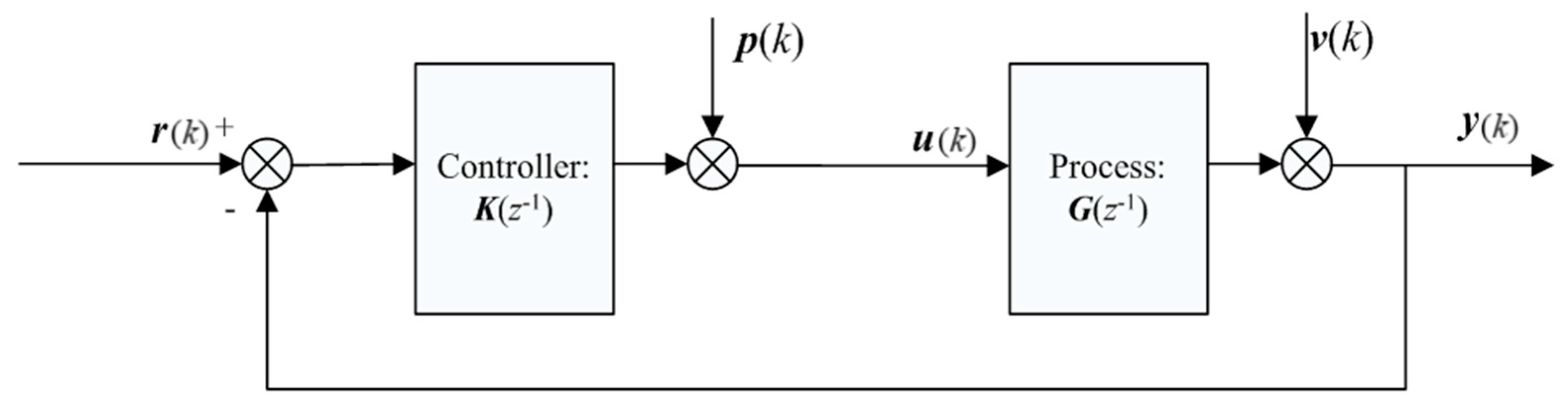
The remainder of this paper is organized as follows. Section 2 introduces the multivariable closed-loop identification object model and the noise model. Section 3 introduces a PCA approach for dealing with the ill-condition problem caused by the correlation of measurement data, and deduces the PALAD identification algorithm. In Section 4, based on PALAD, we analyze the identifiability for multivariable closed-loop systems. 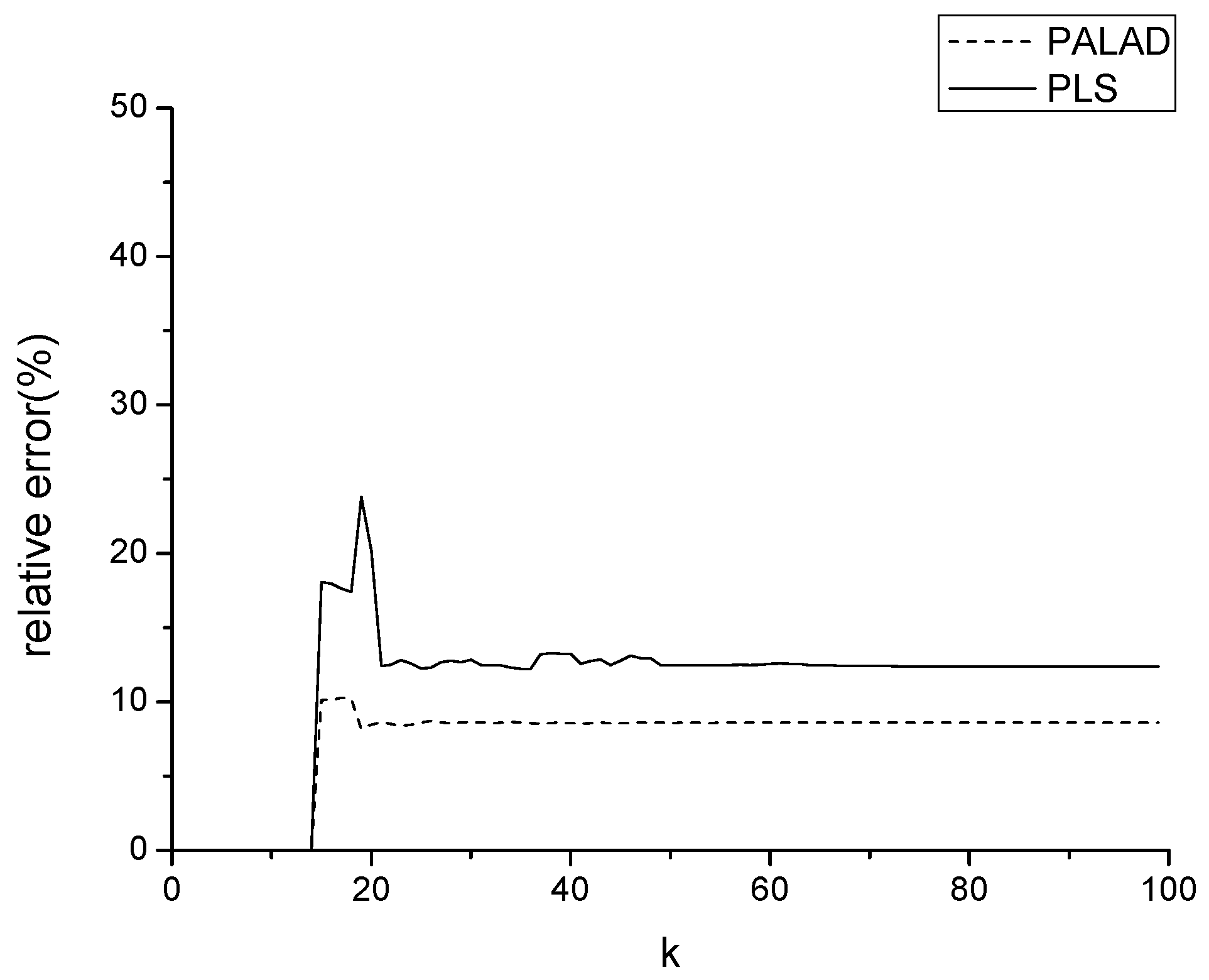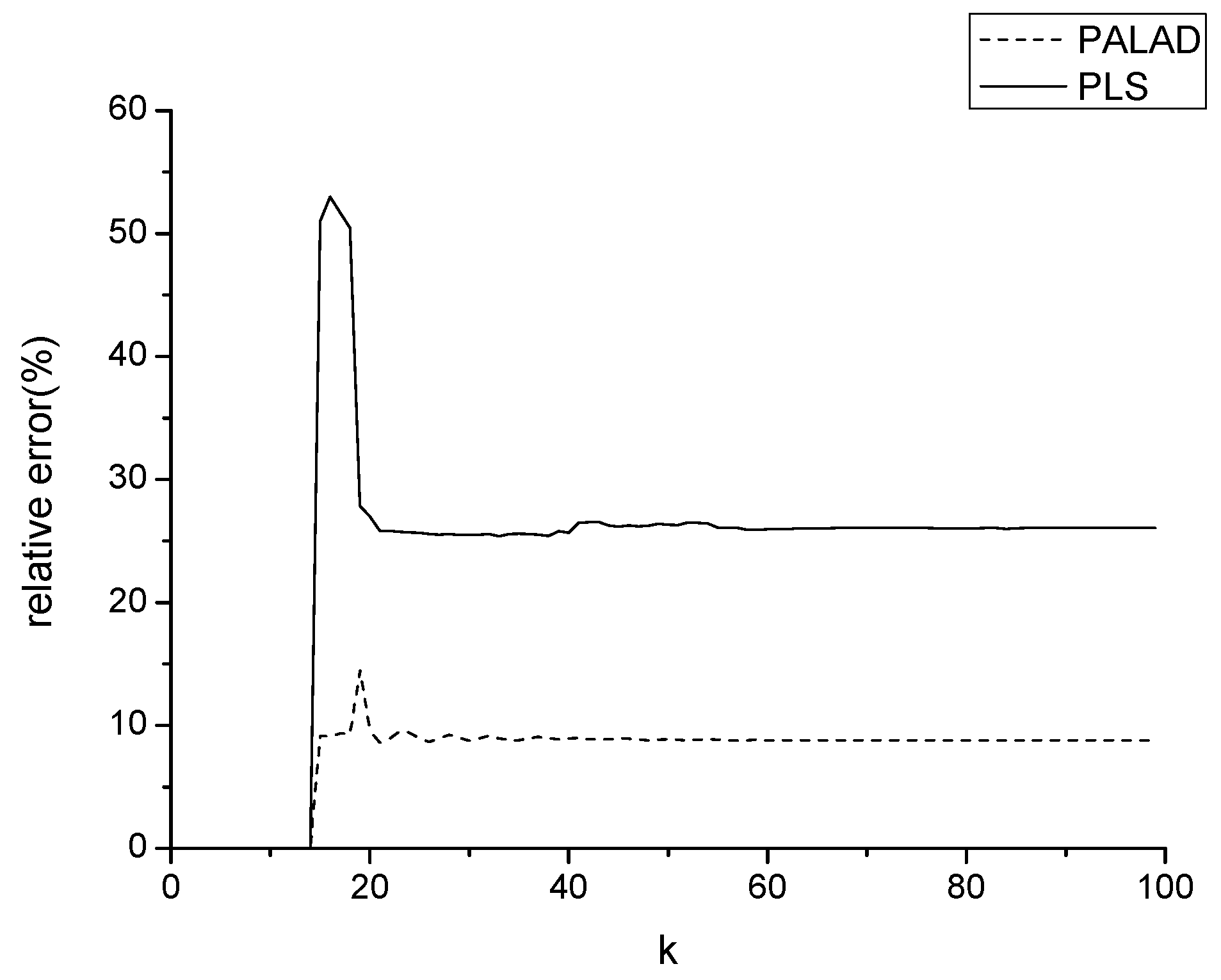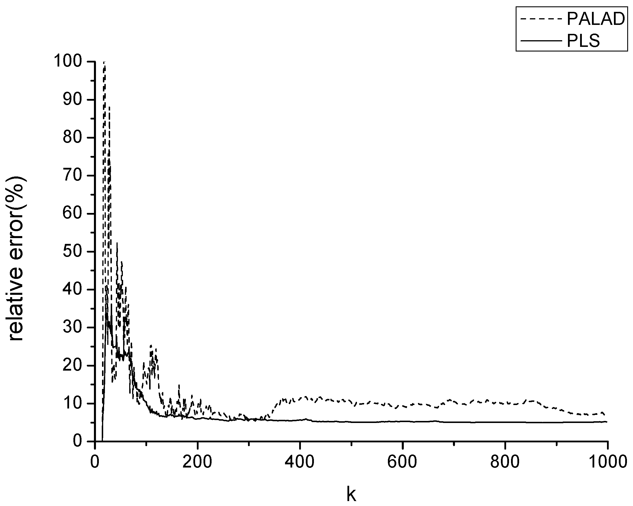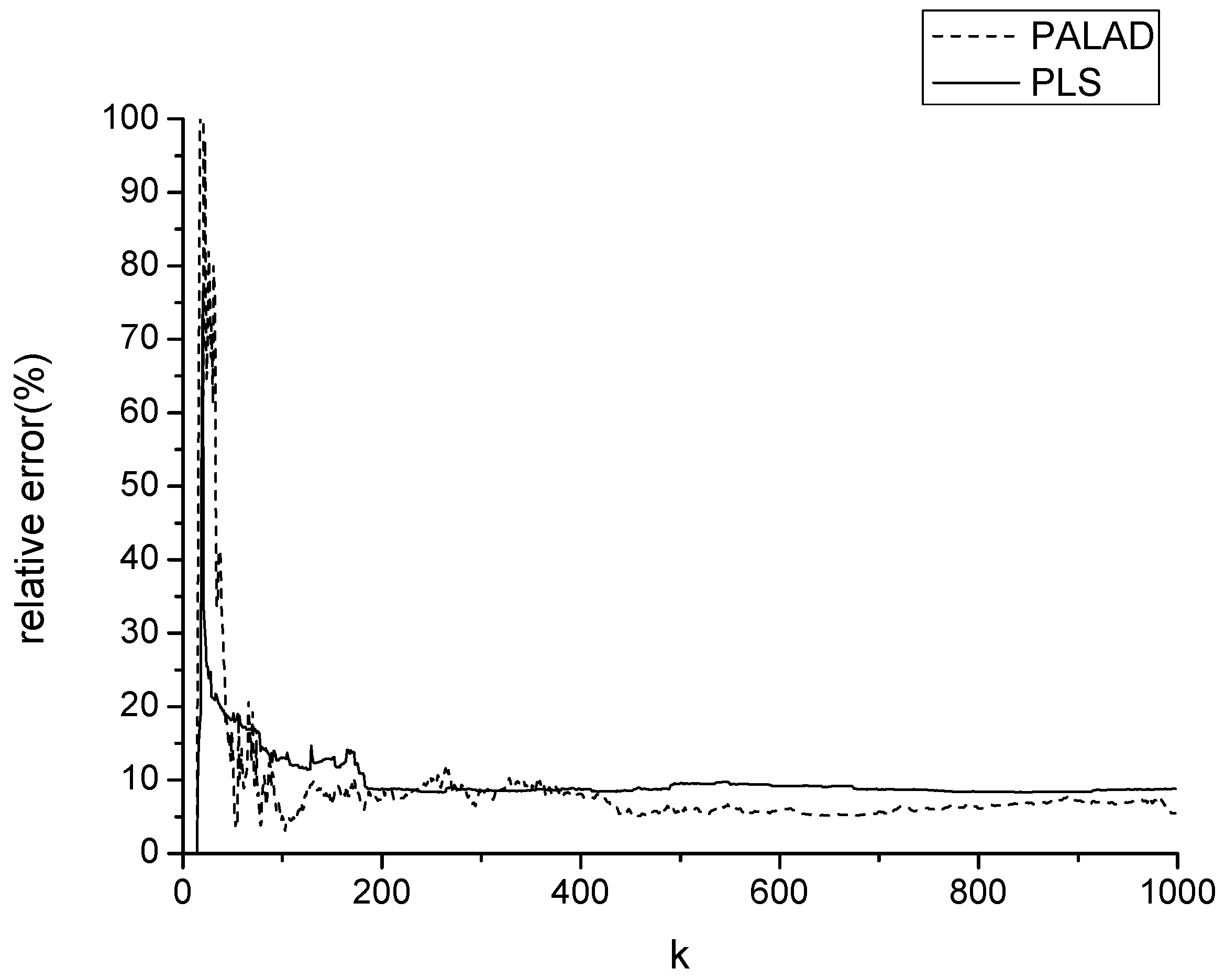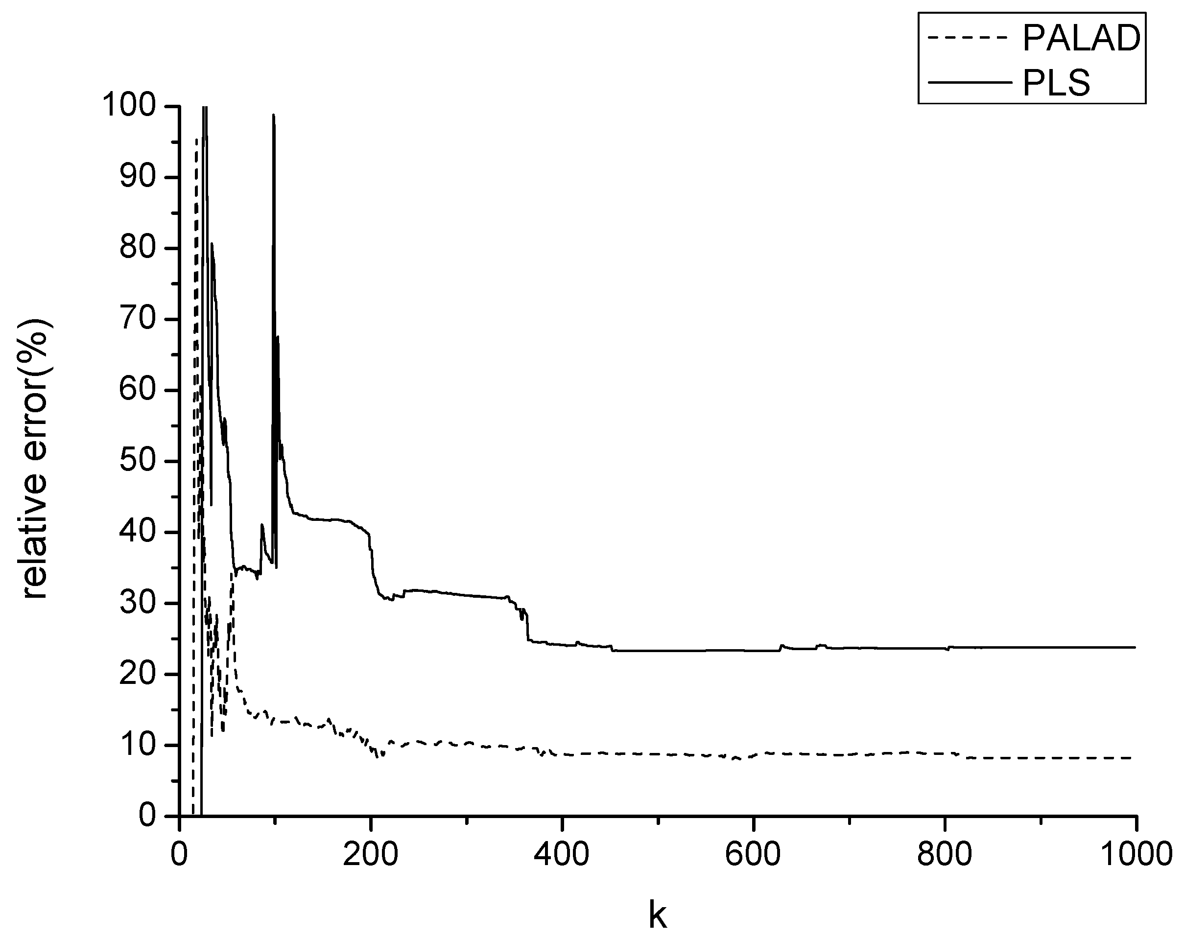According to the modes in Section 2, Section 5 compares the performance of PALAD and PLS identification algorithms. Finally, conclusions are drawn in Section 6.

2. Identification Model

2.1. Multivariable Closed-Loop Identification Object

Figure 1 shows a multivariable linear closed-loop system, where $\mathit{r}(k)\in {\mathit{R}}^s$, $\mathit{u}(k)\in {\mathit{R}}^r$, $\mathit{y}(k)\in {\mathit{R}}^s$, $\mathit{p}(k)$, and $\mathit{v}(k)={[v_1(k),v_2(k),\dots ,v_s(k)]}^{\mathrm{T}}$ denote the reference, input, and process output signals and feedback and forward noises. $\mathit{K}(z^{-1})$ and $\mathit{G}(z^{-1})$ are the transfer functions of the multivariable controller and process plant, respectively.

Let

$$\begin{array}{l}\mathit{K}(z^{-1})=\left[\begin{array}{cccc}{K}_1(z^{-1})& & & \\ & K_2(z^{-1})& & \\ & & \dots & \\ & & & K_s(z^{-1})\end{array}\right],\\ \mathit{B}(z^{-1})=\left[\begin{array}{cccc}{B}_{11}(z^{-1})& B_{12}(z^{-1})& \dots & B_{1r}(z^{-1})\\ B_{21}(z^{-1})& B_{22}(z^{-1})& \dots & B_{2r}(z^{-1})\\ \dots & \dots & \dots & \dots \\ B_{s1}(z^{-1})& B_{s2}(z^{-1})& \dots & B_{sr}(z^{-1})\end{array}\right],\\ A(z^{-1})=1+a_1{z}^{-1}+\dots +a_n{z}^{-n},\\ B_{ij}(z^{-1})=b_{ij}(1)z^{-1}+\dots +b_{ij}(n)z^{-n},\\ P_i(z^{-1})=1+p_i\left(1\right)z^{-1}+\dots +p_i(n)z^{-n},\\ Q_i(z^{-1})=q_i+q_i(1)z^{-1}+\dots +q_i(n)z^{-n},\\ K_i(z^{-1})=Q_i(z^{-1})/P_i(z^{-1}).\end{array}$$

(1)

where $i=1,2,\dots ,s$, $j=1,2,\dots ,r$, and $n$ denotes the model order, and A(z⁻¹), B(z⁻¹), P(z⁻¹), and Q(z⁻¹) are polynomial functions of the delay operator z⁻¹. Denote $\mathit{K}(z^{-1})=\frac{Q(z^{-1})}{P(z^{-1})}$, $\mathit{G}(z^{-1})=\frac{\mathit{B}(z^{-1})}{A(z^{-1})}$. Then, the multiple-input multiple-output (MIMO) linear closed-loop system can be described as in Equation (2).

$$A(z^{-1})\mathit{y}(k)=\mathit{B}(z^{-1})\mathit{u}(k)+\mathit{v}(k)$$

(2)

The direct method in closed loop identification uses $\mathit{u}$ and $\mathit{y}$ to identify multivariable process parameters. Using the coupled identification method, the MIMO closed-loop system is then converted into $s$ multi-input single-output (MISO) closed-loop systems. Let the reference signal $\mathit{r}(k)=0$ and feedback noise $\mathit{p}(k)=0$. The $i$-th MIMO system can be described as

$$\begin{array}{l}\left\{\begin{array}{l}A(z^{-1})y_i(k)={\displaystyle \sum _{j=1}^r{B}_{ij}(z^{-1})u_j(k)}+v_i(k)\\ u_i(k)=-K_i(z^{-1})y_i(k)\end{array}\right.,\\ i=1,2,\dots ,s,\hspace{1em}j=1,2,\dots ,r\end{array}$$

(3)

Let

$$\mathit{\theta }={[{\mathit{a}}^T,{\mathit{\eta }}_1^T,\dots ,{\mathit{\eta }}_s^T]}^T,\mathit{a}={[a(1),a(2),\dots ,a(n)]}^T,$$

$${\mathit{\eta }}_i^T={[{\mathit{b}}_{i1}^T,{\mathit{b}}_{i2}^T,\dots ,{\mathit{b}}_{ir}^T]}^T,{\mathit{b}}_{ij}={[b_{ij}(1),b_{ij}(2),\dots ,b_{ij}(n)]}^T,$$

$$\mathit{y}(k)={[y_1(k),y_2(k),\dots ,y_s(k)]}^T,$$

$$\mathit{\Psi }(k)=[-\mathit{y}(k-1),-\mathit{y}(k-2),\dots ,-\mathit{y}(k-n),{\mathit{I}}_n\otimes {\overline{\mathit{u}}}^T(k)]={[{\mathit{\phi }}_1^T(k),{\mathit{\phi }}_2^T(k),\dots ,{\mathit{\phi }}_s^T(k)]}^T$$

(4)

$$\overline{\mathit{u}}(k)={[{\overline{\mathit{u}}}_1^T(k),{\overline{\mathit{u}}}_2^T(k),\dots ,{\overline{\mathit{u}}}_r^T(k)]}^T,$$

$${\overline{\mathit{u}}}_j(k)={[u_j(k-1),u_j(k-2),\dots ,u_j(k-n)]}^T$$

$$i=1,2,\dots ,s;j=1,2,\dots ,r.$$

Therefore, the MIMO closed-loop system is equivalent to

$$\left\{\begin{array}{l}\mathit{y}(k)=\mathit{\Psi }(k)\mathit{\theta }+\mathit{v}(k)\\ \mathit{u}(k)=-\mathit{K}(z^{-1})\mathit{y}(k)\end{array}\right.$$

(5)

where $\mathit{\Psi }(k)\in {\mathit{R}}^{s\times d}$ is the measured data matrix and $\mathit{\theta }\in {\mathit{R}}^d$ is the parameter to be identified.

The $i$-th subsystem can be described as

$$\begin{array}{l}{y}_i(k)={\mathit{\phi }}_i^T(k)\mathit{\theta }+v_i(k),\\ u_i(k)=K_i(z^{-1})y_i(k),i=1,2,\cdots ,s\end{array}.$$

(6)

2.2. Noise Model

Based on the above system model, two cases of noise model are discussed in the following simulation experiments:

(1)

Only white noise exists in the system;

(2)

White noise coexists with spike noise, obeying $S\alpha S$ distribution.

The spike noise used in this paper obeys an $S\alpha S$ distribution [22], and the probability density function of the standard $S\alpha S$ distribution is

$$f_{\alpha }(x)=\left\{\begin{array}{l}\frac{1}{\pi x}{\displaystyle \sum _{k=1}^{\infty }\frac{{(-1)}^{k-1}}{k!}\Gamma (\alpha k+1){\left|x\right|}^{-\alpha k}\sin (k\alpha \pi /2),0<\alpha <1}\\ \frac{1}{\pi x}{\displaystyle \sum _{k=1}^{\infty }\frac{{(-1)}^k}{2k!}\Gamma \left[(2k+1)/\alpha \right]x^{2k},1<\alpha \le 2}\end{array}\right.$$

(7)

where $\Gamma (*)$ denotes the $\Gamma$ function and $\alpha$ denotes the characteristic exponent. The smaller $\alpha$ is, the higher the probability that the large amplitude sample of the random variable is subjected to the $S\alpha S$ distribution, and the stronger the pulse strength is.

A random variable that is subjected to a standard $S\alpha S$ distribution is obtained through the following steps.

Step 1. Choose a random variable $M$ that obeys a uniform distribution on $\left(-\frac{\pi }{2},\frac{\pi }{2}\right)$.

Step 2. Choose a random variable $N$ that obeys the exponential distribution whose mean value is 1.

Step 3. Choose a variable that obeys the standard $S\alpha S$ distribution by using the following formula:

$$Y=\frac{\sin \alpha M}{{(\cos M)}^{1/\alpha }}{\left(\frac{\cos ((1-\alpha )M)}{N}\right)}^{(1-\alpha )/\alpha }$$

(8)

where $M$ and $N$ are independent.

3. Algorithm Description

The algorithm analysis is based on the $i$-th MISO subsystem for simplicity. Principal component analysis (PCA) is used to obtain the eigenvector $\mathit{\omega }$, which characterizes the measured data vector $\mathit{\Phi }={[{\phi }_i(1),{\phi }_i(2),\dots ,{\phi }_i(m)]}^T$, the principal component vector $\mathit{t}$, and the load matrix $\mathit{P}$ contained in the information of matrix $\mathit{\Phi }$. $m$ is the number of samples. By analyzing the relationship between $\mathit{\Phi }$ and $\mathit{P}$, $\mathit{\Phi }$ is transformed into a full rank matrix $\mathit{P}$, which lays the foundation for solving the unique solution of the linearly related closed-loop system model parameters. Through PCA, the input and output data of the closed-loop system are subjected to partial least absolute regression, and the closed-loop system parameter estimation value is obtained. Given that the LAD function is not differentiable, a deterministic derivative function is introduced to approximately replace the residual absolute value and reduce the computational complexity. We introduce PCA and analyze the relationship between $\mathit{\Phi }$ and $\mathit{P}$. Then, a definite function is selected to approximate the absolute error criterion, considering that the LAD function is non-differentiable. The PALAD recursive algorithm is subsequently derived based on PCA.

3.1. Principal Component Analysis (PCA)

In this research, the PCA method is used to extract the orthogonal principal component from the measurement data, and the extracted principal component can be used in the following identification. PCA can overcome the ill-condition problem caused by the correlation of measurement data. This type of analysis is useful for improving the identifiability of MIMO system identification when linear correlation exists in the measurement data or between input and output data.

In addition to extracting the orthogonal principal component, which contains the data change information of the original independent variable space at the most, PCA also considers the largest interpretation of input variables to output variables when selecting principal components. The following criteria function is proposed:

$$J=\underset{\left|\omega =1\right|}{\min }{\displaystyle \sum _{k=1}^m\left[{‖{\mathit{\phi }}_i(k)-\mathit{\omega }{\mathit{\omega }}^T{\mathit{\phi }}_i(k)‖}^2+{‖y_i(k)-{\mathit{\omega }}^T{\mathit{\phi }}_i(k)‖}^2\right]}$$

(9)

where ${\mathit{\phi }}_i(k)$, $y_i(k)$, $\mathit{\omega }$, and $m$ denote the measured data, output data, principal component weight coefficient vector, and number of samples, respectively. The first item in Equation (5) reflects the requirement that the extracted orthogonal principle component should contain the data change information of the original independent variable space at the most. The second item reflects the requirement that the extracted orthogonal principle component should provide the largest interpretation to the output variables.

Suppose that ${\mathit{\phi }}_i$ and $y_i$ are observed $m$ times, and the data matrices $\mathit{\Phi }\in {\mathit{R}}^{m\times d}$ and $\mathit{Y}\in {\mathit{R}}^{m\times 1}$ are obtained after normalization. PCA is summarized as follows [23]:

(1)

The output data vector $\mathit{Y}$ is considered the initial value of the principal component vector $\mathit{x}$.

(2)

Calculate weight vector $\mathit{\omega }$ of data matrix $\mathit{\Phi }$.

$$\mathit{\omega }={\mathit{x}}^T\mathit{\Phi }/({\mathit{x}}^T\mathit{x})$$

(10)

(3)

Normalize the weight vector $\mathit{\omega }$.

$${\mathit{\omega }}_{new}^T={\mathit{\omega }}^T/‖{\mathit{\omega }}^T‖$$

(11)

(4)

Calculate the principal component vector of $\mathit{\Phi }$.

$$\mathit{t}=\mathit{\Phi }{\mathit{\omega }}_{new}/({\mathit{\omega }}_{new}^T{\mathit{\omega }}_{new})$$

(12)

(5)

Calculate the weight vector of $\mathit{Y}$.

$${\mathit{c}}^T={\mathit{t}}^T\mathit{Y}/({\mathit{t}}^T\mathit{t})$$

(13)

(6)

Normalize the weight vector $\mathit{c}$.

$${\mathit{c}}_{new}^T={\mathit{c}}^T/‖{\mathit{c}}^T‖$$

(14)

(7)

Calculate the principal component vector of $\mathit{Y}$.

$$\mathit{x}=\mathit{Y}{\mathit{c}}_{new}/({\mathit{c}}_{new}^T{\mathit{c}}_{new})$$

(15)

If the principal component vector ${\mathit{t}}_i^{(k)}$ obtained in step (4) is equal to the previous iteration ${\mathit{t}}_i^{(k-1)}$ or the error is less than a predetermined threshold value, then ${\mathit{t}}_i^{(k)}$ has converged to its true value. At this point, step (8) can be performed to calculate the next principal component ${\mathit{t}}_{i+1}$; otherwise, step (2) is implemented and the $k+1$-th iteration is carried out.

(8)

Calculate the load vector for matrix $\mathit{\Phi }$ relative to $\mathit{t}$.

$${\mathit{p}}^T={\mathit{t}}^T\mathit{\Phi }/({\mathit{t}}^T\mathit{t})$$

(16)

(9)

Calculate the load vector for matrix $\mathit{Y}$ relative to $\mathit{t}$.

$${\mathit{q}}^T={\mathit{x}}^T\mathit{Y}/({\mathit{x}}^T\mathit{x})$$

(17)

(10)

Calculate the regression coefficient for $\mathit{x}$ relative to $\mathit{t}$.

$$\beta ={\mathit{x}}^T\mathit{t}/({\mathit{t}}^T\mathit{t})={\mathit{t}}^T\mathit{x}/({\mathit{t}}^T\mathit{t})$$

(18)

(11)

Calculate the residual matrix.

$$\left\{\begin{array}{l}\mathit{E}=\mathit{\Phi }-\mathit{t}{\mathit{p}}^T\\ \mathit{F}=\mathit{Y}-\beta \mathit{t}{\mathit{q}}^T\end{array}\right.$$

(19)

Define $\mathit{\Phi }=\mathit{E}$, $\mathit{Y}=\mathit{F}$. Repeat the above steps and calculate the next principal component until the rank of matrix $\mathit{\Phi }$ is 0. Then, all the principal components are calculated.

3.2. Partial Approximate Least Absolute Deviation (PALAD)

Absolute deviation is not differentiable. To overcome this limitation, we select a deterministic differentiable function to approximate the LAD criterion. This requirement can be met by the following logarithmic function.

$$J(x)=\lambda \ln [\cosh (\frac{x}{\lambda })]$$

(20)

where $\lambda$ is an adjustable parameter and the nonlinear function $J(x)$ is related to $\lambda$. When $\lambda$ is small enough, the nonlinear function $\lambda \ln [\cosh (x/\lambda )]\approx \left|x\right|$, that is, $J(x)\approx \left|x\right|$, approximates the absolute value function. Figure 2 shows the curve of the logarithmic function when $\lambda =0.01$.

Figure 2 shows that the nonlinear function can effectively approximate the absolute value function when $\lambda =0.01$. To enhance the accuracy and robustness of the identification results, the following formula is used as the criteria function for the $i$-th MISO system described in Equation (6).

$$J(\mathit{\theta })={\displaystyle \sum _{k=1}^m\lambda \ln \cosh [\frac{y_i(k)-{\mathit{\phi }}_i{}^T(k)\mathit{\theta }}{\lambda }]}$$

(21)

The recursive formula of $\mathit{\theta }$ is obtained as follows by using the Gauss–Newton method in consideration of the minimization of the objective function (21).

$$\mathit{\theta }(m)=\mathit{\theta }(m-1)+\tau \Delta \mathit{\theta }(m)$$

(22)

where $\tau$ is the learning rate and $\Delta \mathit{\theta }(m)$ is the search direction of the Gauss–Newton method, which is described as

$$\Delta \mathit{\theta }(m)=-{[{\mathit{H}}_m]}^{-1}\mathit{g}(m)$$

(23)

where $\mathit{g}$ denotes the gradient of $J(\mathit{\theta })$ about $\mathit{\theta }$ and $\mathit{H}$ denotes the Hessian matrix of $J(\mathit{\theta })$.

For simplicity, Equation (21) can be rewritten as

$$\begin{array}{l}{J}_m={\displaystyle \sum _{k=1}^m\lambda \ln [\cosh (\frac{y_i(k)-{\mathit{\phi }}_i{}^T(k)\mathit{\theta }}{\lambda })]}\\ =J_{m-1}+\lambda \ln [\cosh (\frac{y_i(m)-{\mathit{\phi }}_i{}^T(m)\mathit{\theta }}{\lambda })]\end{array}$$

(24)

Let $e_i(m)=y_i(m)-{\mathit{\phi }}_i{}^T(m)\mathit{\theta }(m-1)$. Then,

$$J_m=J_{m-1}+\lambda \ln [\cosh (\frac{e_i(m)}{\lambda })]$$

(25)

which leads to

$$\begin{array}{l}\mathit{g}(m)=\frac{\partial J_m}{\partial \mathit{\theta }}\left|{}_{\mathit{\theta }=\mathit{\theta }(m-1)}\right.=\frac{\partial J_{m-1}}{\partial \mathit{\theta }}\left|{}_{\mathit{\theta }=\mathit{\theta }(m-1)}\right.-{\mathit{\phi }}_i(m)\tanh \left[\frac{e_i(m)}{\lambda }\right]\\ =\mathit{g}(m-1)-{\mathit{\phi }}_i(m)\tanh \left[\frac{e_i(m)}{\lambda }\right]\end{array}$$

(26)

$${\mathit{H}}_m=\frac{{\partial }^2{J}_m}{\partial {\mathit{\theta }}^2}=\frac{1}{\lambda }{\displaystyle \sum _{k=1}^m{\mathit{\phi }}_i(k){\mathit{\phi }}_i{}^T(k)\left[1-{\tanh }^2(\frac{e_i(k)}{\lambda })\right]}$$

(27)

The Hessian matrix is symmetrical. To ensure the stability of the algorithm, the positive definite property of the Hessian matrix must be guaranteed to ensure a decent search direction.

$${\mathit{H}}_m=\frac{{\partial }^2{J}_m}{\partial {\mathit{\theta }}^2}={\mathit{H}}_{m-1}+\frac{1}{\lambda }{\mathit{\phi }}_i(m){\mathit{\phi }}_i{}^T(m)[1-{\tanh }^2(\frac{e_i(m)}{\lambda })]$$

(28)

and

$$\begin{array}{l}\Delta \mathit{\theta }(m)=-{[{\mathit{H}}_m]}^{-1}\mathit{g}(m)\\ =-{\left\{\frac{1}{\lambda }{\displaystyle \sum _{k=1}^m{\mathit{\phi }}_i(k){\mathit{\phi }}_i{}^T(k)\left[1-{\tanh }^2(\frac{e_i(k)}{\lambda })\right]}\right\}}^{-1}\left\{\mathit{g}(m-1)-{\mathit{\phi }}_i(m)\tanh [\frac{e_i(m)}{\lambda }]\right\}\end{array}$$

(29)

Then, the recursive formula of the PALAD algorithm is obtained. $\tau$ is the learning rate. $\mathit{\theta }(0)$ and $\Delta \mathit{\theta }(0)$ are initialized by random numbers that are sufficiently small.

4. Identifiability Analysis for Multivariable Closed-Loop Systems

Define the measured data matrix $\mathit{\Phi }\in {\mathit{R}}^{m\times d}$ and output data matrix $\mathit{Y}\in {\mathit{R}}^{m\times 1}$ as normalized matrices. Then, we have

$$\mathit{Y}=\mathit{\Phi }{\mathit{\theta }}_{LS}+\mathit{v}$$

(30)

where ${\mathit{\theta }}_{LS}$ is the least square estimation. ${\mathit{\theta }}_{LS}$ can be described as follows when the order of the feedback channel is higher than that of the forward channel:

$$\left\{\begin{array}{l}{\widehat{\mathit{\theta }}}_{LS}={({\mathit{\Phi }}^T\mathit{\Phi })}^{-1}{\mathit{\Phi }}^T\mathit{Y}\\ ({\mathit{\Phi }}^T\mathit{\Phi }){\widehat{\mathit{\theta }}}_{LS}={\mathit{\Phi }}^T\mathit{Y}\end{array}\right.$$

(31)

If the order of the feedback channel is lower than that of the forward channel and no interference noise exists in the feedback channel, that is, $\mathit{p}(k)=0$, the element $\mathit{u}(k-1)$ of measured data matrix $\mathit{\Phi }$ is linearly related to $\mathit{Y}(k-1),\mathit{Y}(k-2),\cdots ,\mathit{Y}(k-n)$ through the feedback channel, thus confirming that the direct identification method cannot be used to identify parameter ${\mathit{\theta }}_{\mathit{L}\mathit{S}}$. Essentially, matrix ${\mathit{\Phi }}^T\mathit{\Phi }$ is singular, while the elements in matrix $\mathit{\Phi }$ are linearly related. Consequently, ${\widehat{\mathit{\theta }}}_{\mathit{L}\mathit{S}}$ is ill-conditioned and unidentifiable.

For the PALAD algorithm, according to Equation (22),

$$\begin{array}{l}{\mathit{\theta }}_P(m)={\mathit{\theta }}_P(m-1)+\tau \Delta \mathit{\theta }(m)\\ ={\mathit{\theta }}_P(m-1)+\tau \Delta \mathit{\theta }(m)\\ ={\mathit{\theta }}_P(m-1)+\tau \left\{-{[{\mathit{H}}_m]}^{-1}\mathit{g}(m)\right\}\\ ={\mathit{\theta }}_P(m-1)-\tau {\left\{\frac{1}{\lambda }{\displaystyle \sum _{k=1}^m{\mathit{\phi }}_i(k){\mathit{\phi }}_i{}^T(k)\left[1-{\tanh }^2(\frac{e_i(k)}{\lambda })\right]}\right\}}^{-1}\\ \times \left\{\mathit{g}(m-1)-{\mathit{\phi }}_i(m)\tanh [\frac{e_i(m)}{\lambda }]\right\}\end{array}$$

(32)

Let $z_i(k)=\frac{1}{\lambda }\left(1-{\tanh }^2\frac{e_i(k)}{\lambda }\right)$. Then,

$$\begin{array}{l}{\mathit{H}}_m=\frac{{\partial }^2{J}_m}{\partial {\mathit{\theta }}^2}=\frac{1}{\lambda }{\displaystyle \sum _{k=1}^m{\mathit{\phi }}_i(k){\mathit{\phi }}_i{}^T(k)\left[1-{\tanh }^2(\frac{e_i(k)}{\lambda })\right]}\\ ={\displaystyle \sum _{k=1}^m{z}_i(k){\mathit{\phi }}_i(k){\mathit{\phi }}_i{}^T(k)}\\ =\mathit{\Phi }{(m)}^T\mathit{\Phi }(m)\end{array}$$

(33)

where $\mathit{\Phi }{(m)}^T=[\sqrt{z_i(1)}{\mathit{\phi }}_i(1),\sqrt{z_i(2)}{\mathit{\phi }}_i(2),\cdots ,\sqrt{z_i(m)}{\mathit{\phi }}_i(m)]$, ${\mathit{\Phi }}^T\mathit{\Phi }$ is singular, and linear correlations exist in matrix $\mathit{\Phi }$. Thus, ${\mathit{H}}_m$ is a uninvertible matrix, and the closed loop is unidentifiable.

PALAD focuses on eliminating the linear correlation in $\mathit{\Phi }$ and turns a closed-loop unidentifiable system into a closed-loop identifiable system. By mapping the high-dimensional measured and output data spaces onto low-dimensional feature spaces, the eigenvectors of $\mathit{\Phi }$ and $\mathit{Y}$ are obtained. PALAD then establishes the independent linear relationship between the eigenvectors of $\mathit{\Phi }$ and $\mathit{Y}$.

The data matrix $\mathit{\Phi }$ and load matrix $\mathit{P}$ satisfy the following theorem.

Theorem 1.

Assume that matrix $\mathit{\Phi }$ is $m\times d$ if $rank(\mathit{\Phi })=l\le d$. After extracting the  $l$-th eigenvector  $t_l$ , the residual matrix  ${\mathit{E}}_l\in {\mathit{R}}^{m\times l}$  of the independent variable matrix is equal to 0. $t_i$  is defined as the normalized eigenvector; that is,

$${\mathit{\Phi }}^T\mathit{\Phi }={({\mathit{T}}_l{\mathit{P}}_l{}^T+{\mathit{E}}_l)}^T({\mathit{T}}_l{\mathit{P}}_l{}^T+{\mathit{E}}_l)={\mathit{P}}_l{\mathit{P}}_l^T=\mathit{P}{\mathit{P}}^T$$

(34)

where  $\mathit{T}=[{\mathit{t}}_1,{\mathit{t}}_2,\dots ,{\mathit{t}}_l,{\mathit{t}}_{l+1},\dots ,{\mathit{t}}_d]\in {\mathit{R}}^{m\times d}$ ,  ${\mathit{T}}_l=[{\mathit{t}}_1,{\mathit{t}}_2,\dots ,{\mathit{t}}_l]\in {\mathit{R}}^{m\times l}$ ,  $\mathit{P}=[{\mathit{p}}_1,{\mathit{p}}_2,\dots ,{\mathit{p}}_l,{\mathit{p}}_{l+1},\dots ,{\mathit{p}}_d]\in {\mathit{R}}^{d\times d}$, and  ${\mathit{P}}_l=\left[{\mathit{p}}_1,{\mathit{p}}_2,\dots ,{\mathit{p}}_l\right]\in {\mathit{R}}^{d\times l}$.

Proof. 

After extracting $d$ eigenvectors, the residual matrix ${\mathit{E}}_d=0$. Eigenvector ${\mathit{t}}_i$ is a normalized orthogonal vector, which is ${\mathit{T}}^T\mathit{T}={\mathit{I}}_d$. Then,

$$\begin{array}{l}\mathit{\Phi }={\mathit{E}}_0=\mathit{T}{\mathit{P}}^T+{\mathit{E}}_d=\mathit{T}{\mathit{P}}^T\\ {\mathit{\Phi }}^T\mathit{\Phi }=(\mathit{T}{\mathit{P}}^T)\mathit{T}{\mathit{P}}^T=\mathit{P}{\mathit{P}}^T\end{array}$$

if $rank(\mathit{\Phi })=rank(\mathit{T})=l\le d$. After extracting $l$ eigenvectors, the residual matrix of $\mathit{\Phi }$ is ${\mathit{E}}_l=0$, ${\mathit{T}}_l^T{\mathit{T}}_l={\mathit{I}}_l$. Hence, a reduced dimension matrix ${\mathit{P}}_l\in {\mathit{R}}^{d\times l}$ exists that makes

$$\begin{array}{l}\mathit{\Phi }={\mathit{E}}_0={\mathit{T}}_l{\mathit{P}}_l^T+{\mathit{E}}_l={\mathit{T}}_l{\mathit{P}}_l^T\\ {\mathit{\Phi }}^T\mathit{\Phi }={({\mathit{T}}_l{\mathit{P}}_l^T)}^T({\mathit{T}}_l{\mathit{P}}_l^T)={\mathit{P}}_l{\mathit{T}}_l^T{\mathit{T}}_l{P}_l^T={\mathit{P}}_l{\mathit{P}}_l^T\end{array}$$

.

Then,

$${\mathit{P}}_l{\mathit{P}}_l^T=\mathit{P}{\mathit{P}}^T$$

.

The proof is finished. □

According to Equation (33),

$$\begin{array}{l}{\mathit{H}}_m=\frac{{\partial }^2{J}_m}{\partial {\mathit{\theta }}_P{}^2}\\ =\frac{1}{\lambda }{\displaystyle \sum _{k=1}^m{\mathit{\phi }}_i(k){\mathit{\phi }}_i{}^T(k)\left[1-{\tanh }^2(\frac{e_i(k)}{\lambda })\right]}\\ ={\displaystyle \sum _{k=1}^m{z}_i(k){\mathit{\phi }}_i(k){\mathit{\phi }}_i{}^T(k)}\\ ={\mathit{H}}_{m-1}+z_i(m){\mathit{\phi }}_i(m){\mathit{\phi }}_i{}^T(m)\\ ={\mathit{H}}_{m-1}+{\overline{\mathit{\phi }}}_i(m){\overline{\mathit{\phi }}}_i{(m)}^T\end{array},$$

(35)

where ${\overline{\mathit{\phi }}}_i(m)=\sqrt{z_i(m)}{\mathit{\phi }}_i(m)$. According to Theorem 1, data matrix $\mathit{\Phi }(m)$ and load matrix $\mathit{P}(m)$ satisfy the following relationship.

$$\begin{array}{l}\mathit{P}(m){\mathit{P}}^T(m)={\mathit{\Phi }}^T(m)\mathit{\Phi }(m)\\ ={\mathit{\Phi }}^T(m-1)\mathit{\Phi }(m-1)+{\overline{\mathit{\phi }}}_i(m){\overline{\mathit{\phi }}}_i{(m)}^T\\ =\mathit{P}(m-1){\mathit{P}}^T(m-1)+{\overline{\mathit{\phi }}}_i(m){\overline{\mathit{\phi }}}_i{(m)}^T\end{array}$$

(36)

where $\mathit{\Phi }(m)=\left[\begin{array}{c}\mathit{\Phi }(m-1)\\ {\overline{\mathit{\phi }}}_i{(m)}^T\end{array}\right]$.

By comparing Equations (35) and (36), ${\mathit{H}}_m$ can be expressed as

$$\begin{array}{l}{\mathit{H}}_m={\displaystyle \sum _{k=1}^m{z}_i(k){\mathit{\phi }}_i(k){\mathit{\phi }}_i{}^T(k)}\\ =\mathit{\Phi }{(m)}^T\mathit{\Phi }(m)\\ =\mathit{P}(m){\mathit{P}}^T(m)\\ =\mathit{P}(m-1){\mathit{P}}^T(m-1)+{\overline{\mathit{\phi }}}_i(m){\overline{\mathit{\phi }}}_i{}^T(m)\end{array}$$

(37)

where $\mathit{P}(m)$ is the load vector of $\mathit{\Phi }(m)$, which can be calculated using PCA, and $\Delta {\mathit{\theta }}_P$ can be calculated as

$$\begin{array}{l}\Delta {\mathit{\theta }}_P(m)=-[{\mathit{H}}_m]-1\mathit{g}(m)\\ =-[\mathit{P}(m-1){\mathit{P}}^T(m-1)+{\overline{\mathit{\phi }}}_i(m){\overline{\mathit{\phi }}}_i{}^T(m)]-1\left\{\mathit{g}(m-1)-{\mathit{\phi }}_i(m)\tanh [\frac{e_i(m)}{\lambda }]\right\}\end{array}$$

(38)

Therefore, the parameter ${\mathit{\theta }}_P$ is unique, and the identifiability of the closed-loop system is proven.

5. Simulation Experiments

The parameter estimation of the multivariable closed-loop system is only unique and consistent if noise exists in the feedback channel when the order of the feedback channel is lower than that of the forward channel. The absence of noise in the feedback indicates that a correlation exists among the elements of measured data, and the parameters are unsuccessfully identified. The proposed PALAD algorithm eliminates the correlation through PCA, which guarantees the identifiability of the multivariable closed-loop system. Under such circumstances, the identification results of the PALAD algorithm are analyzed under white and different intensity impulse noises, and then compared with those of the LS and PLS algorithms, which are based on the PLS criterion.

5.1. Process with a First-Order Controller

The multivariable closed-loop system process is investigated to confirm the theoretical results obtained above. Consider the system:

$$\left\{\begin{array}{l}A(z^{-1})\mathit{y}(k)=\mathit{B}(z^{-1})\mathit{u}(k)+\mathit{v}(k)\\ \mathit{u}(k)=-\mathit{K}(z^{-1})\mathit{y}(k)\end{array}\right.$$

(39)

$$A(z^{-1})=1+a_1{z}^{-1}+a_2{z}^{-1}=1-1.2z^{-1}-0.6z^{-2}$$

$$\mathit{B}(z^{-1})=\left[\begin{array}{cc}1.1z^{-1}+0.85z^{-2}& 0.6z^{-1}+1.8z^{-2}\\ 0.28z^{-1}+1.21z^{-2}& 1.1z^{-1}+0.85z^{-2}\end{array}\right]$$

where the forward channel is a second-order controller, and the process is controlled by a decentralized first-order controller.

$$\mathit{K}(z)=\left[\begin{array}{cc}0.8-0.6z^{-1}& \\ & 0.8-0.6z^{-1}\end{array}\right]$$

The input sequence $\mathit{u}(k)=\left\{u_1(k),u_2(k)\right\}$ is a series of uncorrelated, continuous, and stochastic sequences with zero mean and unit variance ${\sigma }_{{\mathit{u}}_1}^2={\sigma }_{{\mathit{u}}_2}^2=1$. The noise sequence $v(k)=\left\{v_1(k),v_2(k)\right\}$ is a zero-mean uncorrelated white noise sequence with variance ${\sigma }_{v_1}^2={\sigma }_{v_2}^2=0.1$. The abovementioned MIMO closed-loop system is equivalent to

$$\left\{\begin{array}{l}\mathit{y}(k)=\mathit{\Psi }(k)\mathit{\theta }+\mathit{v}(k)\\ \mathit{u}(k)=-\mathit{K}(z^{-1})\mathit{y}(k)\end{array}\right.$$

(40)

where

$$\mathit{y}(k)={[y_1(k),y_2(k)]}^T$$

$$\mathit{\Psi }(k)=[-\mathit{y}(k-1),-\mathit{y}(k-2),I_2\otimes {\mathit{u}}^T(k)]$$

$$\mathit{\theta }={\left[\begin{array}{cccccccccc}-1.2& -0.6& 1.1& 0.85& 0.6& 1.8& 0.28& 1.21& 1.1& 0.85\end{array}\right]}^T$$

This model generates closed-loop data for the identification procedure. We apply the proposed algorithm to estimate the parameters of this multivariable closed-loop system in different situations. Simulation experiments are performed in MATLAB. To guarantee the reliability of the simulation experiments, independent experiments with data length L = 200 are conducted 100 times for each simulation experiment. The relative error $\delta =\frac{‖\widehat{\mathit{\theta }}(k)-\mathit{\theta }‖}{‖\mathit{\theta }‖}$ is used as the evaluation criterion.

(1)

Simulation result under white noise

White noise with ${\sigma }_{v_1}^2={\sigma }_{v_2}^2=0.1$ is the interfering signal, and part of the estimated parameters and relative error $\delta$ are shown in

Table 1. Experimental results with white noise.

Parameter	${\mathit{\theta }}_{\mathbf{1}}$	${\mathit{\theta }}_{\mathbf{2}}$	${\mathit{\theta }}_{\mathbf{5}}$	${\mathit{\theta }}_{\mathbf{7}}$	${\mathit{\theta }}_{\mathbf{9}}$	${\mathit{\theta }}_{\mathbf{10}}$	${\displaystyle \mathit{\delta }}$(%)
True value	−1.2	−0.6	0.6	0.28	1.1	0.85	0
LS	NaN	NaN	NaN	NaN	NaN	NaN	-
PALAD	−1.2635	−0.7452	0.9047	0.2417	1.2197	0.9160	8.38
PLS	−1.2067	−0.5203	0.9056	0.2684	1.2066	0.8828	4.93

and Figure 3, respectively.

Table 1 shows that PALAD and PLS algorithms can successfully identify the multivariable closed-loop system when the order of the feedback channel is lower than that of the forward channel and noise does not exist in the feedback. On the other hand, the LS algorithm cannot identify the parameters due to the linear correlation in $\mathit{\Phi }$, and the simulation results are consistent with the conclusion. This result demonstrates the effectiveness of the PALAD algorithm in eliminating the correlation between the elements of the measured data $\mathit{\Phi }$ and improving the identifiability of the closed-loop system. The identification accuracy and convergence speed are generally satisfactory. However, the PLS algorithm shows better identification performance than the PALAD algorithm with white noise only.

(2)

Simulation results with simultaneous white and spike noises

A simulation is simultaneously performed with white and impulse noises in the forward channel. To thoroughly analyze the influence of impulse noise, the characteristic index of impulse noise is set to $\alpha =1.5$.

Table 2. Experimental results with white and spike noise when $\alpha =1.5$.

Parameter	${\mathit{\theta }}_1$	${\mathit{\theta }}_2$	${\mathit{\theta }}_5$	${\mathit{\theta }}_7$	${\mathit{\theta }}_9$	${\mathit{\theta }}_{10}$	${\displaystyle \mathit{\delta }}$(%)
True value	−1.2	−0.6	0.6	0.28	1.1	0.85	0
PALAD	−1.2678	−0.7534	0.9201	0.2530	1.2108	0.8808	8.39
PLS	−1.2316	−0.7780	0.8341	0.2913	1.2132	0.8181	8.82

and Figure 4 show the results.

Table 2 and Figure 4 show that PALAD and PLS algorithms obtain satisfactory estimation results for impulse noise. Table 1 and Table 2 show that the relative error of PLS and PALAD algorithms increases from 4.93% to 8.82% and from 8.38% to 8.39%, respectively. PALAD is better at suppressing the impact of spike noise than PLS. The relative error fluctuation is small; that is, the PALAD algorithm shows strong robustness against impulse noise.

In terms of the $S\alpha S$ distribution function, the smaller the value of the characteristic index, the higher the probability of the large sample of impulse noise. To further verify the robustness of the PALAD algorithm, we reduce the value of the characteristic index in the following simulation experiment. The model is simulated when $\alpha =1.2$ and $\alpha =0.9$, and then compared with the identification results when $\alpha =1.5$. The results are presented as follows.

With the decrease in characteristic index $\alpha$, the pulse characteristic of the spike noise increases, and the interference of the spike noise signal to the multivariable closed-loop system increases. Figure 5 and Figure 6 show that the accuracy of the PALAD algorithm decreases when $\alpha =1.2$ and $\alpha =0.9$. The gradually enhanced noise signal exerts a great impact on the identification result, which is consistent with practical situations. However, the relative error of PALAD fluctuates only in a small range when the noise interference signal are considerably changed. It increases from 8.59% to 8.79% in

Table 3. Experimental results with white and spike noise when $\alpha =1.2$.

Parameter	${\mathit{\theta }}_1$	${\mathit{\theta }}_2$	${\mathit{\theta }}_5$	${\mathit{\theta }}_7$	${\mathit{\theta }}_9$	${\mathit{\theta }}_{10}$	$\mathit{\delta }$(%)
True value	−1.2	−0.6	0.6	0.28	1.1	0.85	0
PALAD	−1.2715	−0.7577	0.9248	0.2574	1.2119	0.8910	8.59
PLS	−1.1160	−0.3220	0.7934	0.2904	1.2132	0.8201	12.38

and

Table 4. Experimental results with white and spike noise when $\alpha =0.9$.

Parameter	${\mathit{\theta }}_1$	${\mathit{\theta }}_2$	${\mathit{\theta }}_5$	${\mathit{\theta }}_7$	${\mathit{\theta }}_9$	${\mathit{\theta }}_{10}$	$\mathit{\delta }$(%)
True value	−1.2	−0.6	0.6	0.28	1.1	0.85	0
PALAD	−1.2449	−0.7579	0.8885	0.2869	1.2326	0.9450	8.79
PLS	−1.0861	−0.4023	0.6834	0.3752	1.2370	0.5809	26.05

. However, the identification accuracy decreases substantially when the PLS algorithm is used. The relative error increases from 12.38% to 26.05%, indicating that the PLS algorithm cannot accurately identify the parameters, and the effect of spike noise intensifies. Therefore, the PALAD algorithm can eliminate the correlation existing in the measured data of the multivariable and effectively suppress impulse noise, further revealing its strong robustness.

5.2. Process with a Zero-Order Controller

Further research on the decorrelation of the multivariable closed-loop system is performed to demonstrate the accuracy and effectiveness of PALAD. In this case, 100 repeats of independent experiments with data length L = 1000 are conducted for each simulation experiment. The multivariable closed-loop system process pertains to the same process:

$$\left\{\begin{array}{l}A(z^{-1})\mathit{y}(k)=\mathit{B}(z^{-1})\mathit{u}(k)+\mathit{v}(k)\\ \mathit{u}(k)=-\mathit{K}(z^{-1})\mathit{y}(k)\end{array}\right.$$

$$A(z^{-1})=1+a_1{z}^{-1}+a_2{z}^{-1}=1-1.2z^{-1}-0.6z^{-2}$$

$$\mathit{B}(z^{-1})=\left[\begin{array}{cc}1.1z^{-1}+0.85z^{-2}& 0.6z^{-1}+1.8z^{-2}\\ 0.28z^{-1}1.21z^{-2}& 1.1z^{-1}0.85z^{-2}\end{array}\right].$$

This process is controlled by a decentralized zero-order controller:

$$\mathit{K}(z)=\left[\begin{array}{cc}0.5& \\ & 0.5\end{array}\right].$$

The abovementioned MIMO closed-loop system is equivalent to

$$\left\{\begin{array}{l}\mathit{y}(k)=\mathit{\Psi }(k)\mathit{\theta }+\mathit{v}(k)\\ \mathit{u}(k)=\mathit{K}(z^{-1})\mathit{y}(k)\end{array}\right.,$$

(41)

where

$$\mathit{y}(k)={[y_1(k),y_2(k)]}^T$$

$$\mathit{\Psi }(k)=[-\mathit{y}(k-1),-\mathit{y}(k-2),I_2\otimes {\mathit{u}}^T(k)]$$

$$\mathit{\theta }={\left[\begin{array}{cccccccccc}-1.2& -0.6& 1.1& 0.85& 0.6& 1.8& 0.28& 1.21& 1.1& 0.85\end{array}\right]}^T.$$

(1)

Simulation results under white noise

White noise ${\sigma }_{v_1}^2={\sigma }_{v_2}^2=0.1$ is the interfering signal.

Table 5. Experimental results with white noise.

Parameter	${\mathit{\theta }}_1$	${\mathit{\theta }}_2$	${\mathit{\theta }}_5$	${\mathit{\theta }}_7$	${\mathit{\theta }}_9$	${\mathit{\theta }}_{10}$	${\displaystyle \mathit{\delta }}$(%)
True value	−1.2	−0.6	0.6	0.28	1.1	0.85	0
PALAD	−1.2507	−0.6386	0.8900	0.4558	1.2745	0.7944	6.82
PLS	−1.2616	−0.6629	0.9323	0.2794	1.1437	0.8108	5.22

and Figure 7 show the results and relative error $\delta$, respectively.

(2)

Simulation results with simultaneous white and spike noises

We reduce the value of the characteristic index in the following simulation experiment.

Table 6. Experimental results with white and spike noise when $\alpha =1.5$.

Parameter	${\mathit{\theta }}_1$	${\mathit{\theta }}_2$	${\mathit{\theta }}_5$	${\mathit{\theta }}_7$	${\mathit{\theta }}_9$	${\mathit{\theta }}_{10}$	${\displaystyle \mathit{\delta }}$(%)
True value	−1.2	−0.6	0.6	0.28	1.1	0.85	0
PALAD	−1.2041	−0.6592	0.9178	0.2274	1.1052	0.9143	5.90
PLS	−1.1796	−0.6670	1.0627	0.2600	1.2684	0.9114	8.85

,

Table 7. Experimental results with white and spike noise when $\alpha =1.2$.

Parameter	${\mathit{\theta }}_1$	${\mathit{\theta }}_2$	${\mathit{\theta }}_5$	${\mathit{\theta }}_7$	${\mathit{\theta }}_9$	${\mathit{\theta }}_{10}$	$\mathit{\delta }$(%)
True value	−1.2	−0.6	0.6	0.28	1.1	0.85	0
PALAD	−1.2132	−0.4946	0.6643	0.2682	1.2137	0.8119	7.53
PLS	−1.1951	−0.4522	0.5606	0.3584	1.2276	0.5756	14.30

and

Table 8. Experimental results with white and spike noise when $\alpha =0.9$.

Parameter	${\mathit{\theta }}_1$	${\mathit{\theta }}_2$	${\mathit{\theta }}_5$	${\mathit{\theta }}_7$	${\mathit{\theta }}_9$	${\mathit{\theta }}_{10}$	$\mathit{\delta }$(%)
True value	−1.2	−0.6	0.6	0.28	1.1	0.85	0
PALAD	−1.1453	−0.4889	0.6409	0.2834	1.2150	0.7808	8.25
PLS	−1.1686	−0.9447	1.4450	0.2844	1.1067	1.1798	23.82

and Figure 8, Figure 9 and Figure 10 show the results when $\alpha =1.5$, $\alpha =1.2$, and $\alpha =0.9$.

The simulation results show that the PALAD algorithm can still accurately identify the model parameters when the controller is of zero-order, which is consistent with the previous conclusion.

6. Conclusions

In this study, the PALAD algorithm is proposed for a multivariable closed-loop system whose model order of the feedback channel is lower than that of the forward channel and where no noise exists in the feedback channel. It is worth mentioning that the method proposed in this paper is based on the premise of sufficient excitation signals, the determination of the noise model class, and the linear identification process. It is not universal for all industrial processes, which is also a problem in the practical engineering application of multivariate process identification theory. The PCA method is adopted to eliminate the linear correlation existing in the elements of the data vector. The proposed method is based on the PALAD algorithm, which demonstrates superiority in solving non-differentiable problems. The identifiability of the multivariable closed-loop system is proven theoretically. The results demonstrate that the PALAD algorithm can effectively eliminate the linear correlation and accurately identify the parameters for the multivariable closed-loop system when the model order of feedback is lower than that of the forward channel and no noise exists in the feedback channel. In addition, the PALAD algorithm considerably improves accuracy and effectively suppresses spike noise that obeys the $S\alpha S$ distribution.

References

1. Gu, Q.Y.; Hoo, K.A. Model-based closed-loop control of the hydraulic fracturing process. Ind. Eng. Chem. Res. 2015, 54, 1585–1594. [Google Scholar] [CrossRef]
2. Krättli, M.; Ströhlein, G.; Aumann, L.; Müller-Späth, T.; Morbidelli, M. Closed loop control of the multi-column solvent gradient purification process. J. Chromatogr. A 2011, 1218, 9028–9036. [Google Scholar] [CrossRef] [PubMed]
3. Ljung, L. System Identification Theory for the User, 2nd ed.; Prentice Hall: Englewood Cliffs, NJ, USA, 1999. [Google Scholar]
4. Fang, C.Z.; Xiao, D.Y. Process Identification; Tsinghua University Press: Beijing, China, 1988. [Google Scholar]
5. Gevers, M.; Bazancella, A.; Miskovic, L. Informative data: How to get just sufficiently rich? In Proceedings of the IEEE Conference on Decision & Control, Cancun, Mexico, 9–11 December 2008; Volume 16, pp. 1962–1967. [Google Scholar]
6. Uematsu, R.; Masuda, S.; Kano, M. Closed-loop identification of plant and disturbance models based on data-driven generalized minimum variance regulatory control. J. Process Control 2022, 115, 197–208. [Google Scholar] [CrossRef]
7. Zhu, Y.; Yan, W.G.; Zhu, Y.C. MPC closed-loop identification without excitation. J. Process Control 2021, 106, 122–129. [Google Scholar] [CrossRef]
8. Vau, B.; Bourlès, H. Closed-loop output error identification algorithms with predictors based on generalized orthonormal transfer functions: Convergence conditions and bias distribution. Automatica 2021, 125, 109377. [Google Scholar] [CrossRef]
9. Shardt, Y.A.W.; Huang, B. Closed-loop identification condition for ARMAX models using routine operating data. Automatica 2011, 47, 1534–1537. [Google Scholar] [CrossRef]
10. Gupta, R.D.; Fairman, F. Parameter estimation for multivariable systems. IEEE Trans. Autom. Control 1974, 19, 546–549. [Google Scholar] [CrossRef]
11. Mei, H.; Li, S. Decentralized identification for multivariable integrating processes with time delays from closed loop step tests. ISA Trans. 2007, 46, 189–198. [Google Scholar] [CrossRef] [PubMed]
12. Zhang, X.Y.; Hoagg, J.B. Subsystem identification of multivariable feedback and feedforward systems. Automatica 2016, 72, 131–137. [Google Scholar] [CrossRef]
13. Ding, F.; Chen, T. Identification of Hammerstein nonlinear ARMAX system. Automatica 2005, 41, 361–396. [Google Scholar] [CrossRef]
14. Chintakindi, S.; Alsamhan, A.; Abidi, M.H.; Kumar, M.P. Annealing of Monel 400 Alloy Using Principal Component Analysis, Hyper-parameter Optimization, Machine Learning Techniques, and Multi-objective Particle Swarm Optimization. Int. J. Comput. Intell. Syst. 2022, 15, 18. [Google Scholar] [CrossRef]
15. Beyaztas, U.; Han, L.S. A robust functional partial least squares for scalar-on-multiple-function regression. J. Chemom. 2022, 36, e3394. [Google Scholar] [CrossRef]
16. Lauri, D.; Salcedo, J.; Garcia-Nieto, S.; Martinez, M. A PLS approach to identifying predictive ARX models. In Proceedings of the 2009 IEEE Control Applications & Intelligent Control, St. Petersburg, Russia, 8–10 July 2009. [Google Scholar]
17. Xu, B.C.; Liu, X.L. Research on identification algorithm based on the approximate least absolute deviation criteria. Int. J. Autom. Comput. 2012, 8, 501–505. [Google Scholar] [CrossRef]
18. Xu, B.C.; Zhang, Y.D. Multi-innovation identification algorithm based on approximate least absolute deviation. Control Eng. China 2015, 22, 60–65. [Google Scholar]
19. Xiang, H.; Chen, Z.H. New identification method of nonlinear systems based on Hammerstein models. Control Theory Appl. 2007, 24, 143–147. [Google Scholar]
20. Dong, J.; Xie, K.G. Research of the Non-Linear Regress Models Based on the Least Absolute Criteria. J. Chongqing Norm. Univ. (Nat. Sci. Ed.) 2001, 18, 71–74. [Google Scholar]
21. Dong, Q. Relaxation Algorithm Based on ‘Least Absolute Deviation’ Criterion. Predict Method Res. 1990, 9, 16–18. [Google Scholar]
22. Coates, M.J.; Kuruoglu, E. Time-frequency based detection in impulsive noise environments using alpha-stable noise model. Digit. Signal Process. 2002, 82, 1917–1925. [Google Scholar] [CrossRef]
23. Wang, G.Z.; Ye, H. Principal Component Analysis and Partial Least Squares; Tsinghua University Press: Beijing, China, 2012. [Google Scholar]
Figure 1. Multivariable closed-loop system.
Processes 11 03262 g001
Figure 2. Curve of the function property when λ = 0.01 .
Processes 11 03262 g002
Figure 3. Curves of the relative error with white noise.
Processes 11 03262 g003
Figure 4. Curves of the relative error when α = 1.5 .
Processes 11 03262 g004
Figure 5. Curves of the relative error when α = 1.2 .
Processes 11 03262 g005
Figure 6. Curves of the relative error when α = 0.9 .
Processes 11 03262 g006
Figure 7. Curves of the relative error with white noise.
Processes 11 03262 g007
Figure 8. Curves of the relative error when α = 1.5 .
Processes 11 03262 g008
Figure 9. Curves of the relative error when α = 1.2 .
Processes 11 03262 g009
Figure 10. Curves of the relative error when α = 0.9 .
Processes 11 03262 g010