A Novel Hybrid Deep Learning Model for Forecasting Ultra-Short-Term Time Series Wind Speeds for Wind Turbines

Abstract

Accurate forecasting of ultra-short-term time series wind speeds (UTSWS) is important for improving the efficiency and safe and stable operation of wind turbines. To address this issue, this study proposes a VMD-AOA-GRU based method for UTSWS forecasting. The proposed method utilizes variational mode decomposition (VMD) to decompose the wind speed data into temporal mode components with different frequencies and effectively extract high-frequency wind speed features. The arithmetic optimization algorithm (AOA) is then employed to optimize the hyperparameters of the model of the gated recurrent unit (GRU), including the number of hidden neurons, training epochs, learning rate, learning rate decay period, and training data temporal length, thereby constructing a high-precision AOA-GRU forecasting model. The AOA-GRU forecasting model is trained and tested using different frequency temporal mode components obtained from the VMD, which achieves multi-step accurate forecasting of the UTSWS. The forecasting results of the GRU, VMD-GRU, VMD-AOA-GRU, LSTM, VMD-LSTM, PSO-ELM, VMD-PSO-ELM, PSO-BP, VMD-PSO-BP, PSO-LSSVM, VMD-PSO-LSSVM, ARIMA, and VMD-ARIMA are compared and analyzed. The calculation results show that the VMD algorithm can accurately mine the high-frequency components of the time series wind speed, which can effectively improve the forecasting accuracy of the forecasting model. In addition, optimizing the hyperparameters of the GRU model using the AOA can further improve the forecasting accuracy of the GRU model.

1. Introduction

With the gradual depletion of fossil fuels and the continuous increase in energy demand arising from human societal development, wind power has been extensively developed and utilized as a renewable energy source in recent years [1]. According to the “Global Wind Report 2023” released by the Global Wind Energy Council (GWEC), global wind power added 78 GW of installed capacity in 2022, reaching a total installed capacity of 906 GW [2]. Wind speed is the primary factor affecting the operational characteristics of wind turbines, and its randomness, intermittency, and volatility pose a significant challenge for the optimal operation of wind turbines [3,4]. Accurate forecasting of the distribution characteristics of short-term wind speeds is an effective means of improving the safety and economic efficiency of wind turbine operations.

Based on the different timescales of wind speed forecasting, time series wind speed forecasting can be divided into three categories: ultra-short-term forecasting, short-term forecasting, and medium-to-long-term forecasting [5]. Time series wind speed forecasting methods can be classified into statistical forecasting methods, artificial intelligence forecasting methods, and hybrid forecasting methods based on the forecasting mechanism employed [6,7]. Statistical forecasting methods use statistical models to extract the historical features of time series wind speeds and forecast future wind speeds based on these features. Commonly used statistical forecasting models include the AR model [8,9], ARMA model [10,11,12], and ARIMA [13,14,15]. Statistical forecasting models exhibit good forecasting performance when the historical data are sufficient and relatively stable. However, their forecasting capability tends to degrade when dealing with incomplete historical data or non-stationary data. Especially with time series data with random distribution characteristics, the predictive performance of statistical prediction models is difficult to meet the prediction needs.

With the rapid development of artificial intelligence technology, its application to time series wind speed forecasting has received considerable attention in terms of research and applications [16,17]. Machine learning, with its strong capability for nonlinear mapping, has demonstrated excellent performance in wind speed forecasting [18,19,20]. In a previous study [21], a novel hybrid model was developed for short-term wind speed forecasting, and the calculation results illustrated that the proposed hybrid model outperformed single and recently developed forecasting models. A complete ensemble empirical mode decomposition with adaptive noise-least absolute shrinkage and selection operator-quantile regression neural network (CEEMDAN-LASSO-QRNN) model was developed for multistep wind speed probabilistic forecasting [22], and the experimental results indicated a higher accuracy and robustness of the proposed model in multistep wind speed probabilistic forecasting. Yang et al. [23] developed an innovative ensemble system based on mixed-frequency modeling to perform wind speed point and interval forecasting, and a multi-objective optimizer-based ensemble forecaster was proposed to provide deterministic and uncertain information regarding future wind speeds. The calculation results demonstrated that the system outperformed the benchmark techniques and could be employed for data monitoring and analysis on wind farms. Dong et al. [24] proposed an ensemble system of decomposition, adaptive selection, and forecasting to simulate the actual wind speed data of a wind farm. The calculation results indicated that the proposed forecasting model had outstanding forecasting accuracy for time series wind speeds. Machine learning methods can explore the nonlinear relationships of data, but they cannot explore the spatiotemporal distribution characteristics between data, resulting in low accuracy of machine learning methods in predicting time series data.

Deep learning exhibits exceptional capabilities in nonlinear mapping and time series data analysis, leading to superior performance in time series wind speed forecasting [25,26]. For instance, Lv et al. [27] applied a deep learning model to forecast time series wind speeds after removing data noise. The computational results demonstrated that the proposed method could accurately forecast time series wind speed sequences. A dynamic adaptive spatiotemporal graph neural network (DASTGN) was proposed for forecasting wind speed, and extensive experiments on real wind speed datasets in the Chinese seas showed that DASTGN improved the performance of the optimal baseline model by 3.05% and 3.69% in terms of MAE and RMSE, respectively [28]. A wind speed forecasting model based on hybrid variational mode decomposition (VMD), improved complete ensemble empirical mode decomposition with additive noise (ICEEMDAN), and a long short-term memory (LSTM) neural network has also been proposed [29]. By comparing and analyzing seven other forecasting models, the proposed model was found to have the best forecasting accuracy. Other studies [26,30,31,32,33] have presented a novel transformer-based deep neural network architecture integrated with a wavelet transform for forecasting wind speed and wind energy (power) generation for 6 h in the future, and the calculation results demonstrated that the integration of the transformer model with wavelet decomposition improved the forecasting accuracy. A single deep learning model can only explore the distribution characteristics (spatial or temporal distribution characteristics) of a certain aspect of data, and cannot simultaneously explore the spatiotemporal distribution and coupling characteristics of data. Therefore, a hybrid forecasting model with spatial and temporal feature mining capabilities is an effective method to improve the accuracy of ultra-short-term wind speed forecasting.

Integrating the advantages of different deep learning models to construct hybrid forecasting models can effectively overcome the limitations of individual deep learning forecasting models and further improve wind speed forecasting accuracy [34,35]. A hybrid forecasting model was developed by combining the strengths of a convolutional neural network (CNN) model and a bidirectional long short-term memory (BiLSTM) model, and was then applied to short-term wind speed forecasting [36,37]. The computational results demonstrated that the hybrid CNN-BiLSTM forecasting model could accurately capture the spatiotemporal distribution characteristics of wind speed information, leading to a higher forecasting accuracy than that of individual deep learning models. Assigning different weights to multiple deep learning models for ensemble construction in short-term wind speed forecasting allows each model’s strengths to be fully utilized, thereby enhancing the overall forecasting accuracy of the ensemble model and expanding its practical applicability [38].

Based on an existing study on wind speed forecasting, this study presents a forecasting model based on VMD-AOA-GRU for ultra-short-term time series wind speed (UTSWS). In the proposed model, historical wind speed data from wind turbines were first decomposed into different frequency sub-sequences using variational mode decomposition (VMD). Then, the arithmetic optimization algorithm (AOA) was utilized to optimize the temporal length of the training data for each sub-sequence and the hyperparameters of the forecasting model of the gated recurrent unit (GRU), such as the number of hidden neurons, training epochs, learning rate, and learning rate decay period, to improve the convergence speed and forecasting accuracy of the GRU model. Finally, the forecasting accuracies of various hybrid forecasting models were compared to demonstrate the superiority of the proposed algorithm.

Compared with existing wind speed forecasting models, our proposed model has the following advantages:

(1)

A UTSWS forecasting model based on VMD-AOA-GRU is proposed.

(2)

VMD is employed to extract high-frequency wind speed features from time series wind speeds.

(3)

The hyperparameters of the GRU model are optimized using the AOA to construct a hybrid AOA-GRU model.

(4)

The proposed model outperforms other models for the four wind speed datasets.

The remainder of this paper is organized as follows: In Section 2, the principles of time series wind speed forecasting are introduced. The computational principles and decomposition process of VMD are presented in Section 3. The computational principles and process of the AOA are described in Section 4, including the calculation process for the accelerated function of the math optimizer, the global exploration phase, and the local exploitation phase. Section 5 describes the construction process for the AOA-GRU hybrid model, including the principles of GRU and the construction of the AOA-GRU model. The construction and validation processes for the VMD-AOA-GRU model are outlined in Section 6. In Section 7, the multi-step forecasting results of various models are compared, including GRU, VMD-GRU, VMD-AOA-GRU, LSTM, VMD-LSTM, PSO-ELM, VMD-PSO-ELM, PSO-BP, VMD-PSO-BP, PSO-LSSVM, VMD-PSO-LSSVM, ARIMA, and VMD-ARIMA. The results of this study are summarized in Section 8.

2. Principles of Time Series Wind Speed Forecasting

Wind speed sequences are essentially time series data, and for a specific wind farm, the wind speed time series can vary significantly under different climatic conditions. We assume that a set of real wind speed time series is denoted as A_k = {a₁, a₂, a₃, …, a_k}, where a_k represents the wind speed at the k^th time step. Then, the wind speed, a_k+1, at the (k + 1)^th time step can be calculated using Equation (1).

$$a_{k+1}=f\left(A_k\right)=f\left(a_1,a_2,\cdots ,a_{k-1},a_k\right),$$

(1)

where f(·) represents the forecasting model, and k represents the length of the sliding time window.

Equation (1) expresses single-step wind speed forecasting. The principle of multi-step forecasting of time series wind speeds is similar to that of single-step forecasting. Taking two-step forecasting as an example, the wind speed, a_k+2, at time k + 2 can be calculated using Equation (2).

$$a_{k+2}=f\left(a_2,a_3,\cdots ,a_k,a_{k+1}\right)$$

(2)

In Equation (2), the wind speed sequence {a₁, a₂, a₃, …, a_k} is shifted one step to the left, and the forecasting value a_k+1 at time k + 1 is then added to the wind speed sequence as an input to the forecasting model. Similarly, the predicted value a_k+n at time k + n can be calculated using Equation (3).

$$a_{k+n}=f\left(a_n, a_{n+1}, \cdots , a_{k+(n-2)}, a_{k+(n-1)}\right)$$

(3)

As indicated by the above equations, in time series wind speed forecasting, as the forecasting step increases, the forecasting error will accumulate with each step in the forecasting model, f(·), leading to a decrease in forecasting accuracy.

The principle of time series wind speed forecasting is illustrated in Figure 1.

3. Variational Mode Decomposition

VMD is a non-stationary signal decomposition method introduced by Dragomiretskiy et al. in 2014 [39]. VMD achieves signal decomposition by introducing variational constraints, thus effectively overcoming the mode mixing and endpoint effects issues present in traditional empirical mode decomposition (EMD) methods.

VMD assumes that any signal f(t) can be represented by a series of sub-signals u_k with specific center frequencies and finite bandwidths, and the sum of the bandwidths of all of the sub-signals is equal to the original signal. Then, the variational constraint equation shown in Equation (4) can be obtained.

$$\{\begin{array}{c}\underset{\left\{u_k\right\},\left\{{\omega }_k\right\}}{\min }\left\{{\displaystyle \sum _k{\Vert {\partial }_t\left[(\delta (t)+j/\pi \cdot t)\otimes u_k(t)\right]e^{-i{\omega }_{k}t}\Vert }_2^2}\right\}\\ \mathrm{s}.\mathrm{t}.{\displaystyle \sum _{k=1}^K{u}_k}=f(t)\end{array}$$

(4)

In Equation (4), K represents the number of variational modes, {u_k, ω_k} represents the k^th decomposed mode component with its corresponding center frequency, ∂_t is the partial derivative with respect to time t, δ(t) represents the Dirac function, and ⊗ represents the convolution operator.

To transform a constrained variational problem into a non-constrained variational problem, VMD introduces quadratic penalty factors, α, and Lagrange multipliers, λ(t), to construct the augmented Lagrangian function L({u_k}, {ω_k}, λ), thereby converting the constrained problem into an unconstrained one. The constructed Lagrangian function is expressed in Equation (5).

$$\begin{array}{c}L\left(\left\{u_k\right\},\left\{{\omega }_k\right\},\lambda \right)=\alpha {\displaystyle \sum _{k=1}^K{\Vert {\partial }_t\left[(\delta (t)+j/\pi \cdot t)\otimes u_k(t)\right]e^{-i{\omega }_{k}t}\Vert }_2^2}\\ +{\Vert f(t)-{\displaystyle \sum _{k=1}^K{u}_k}(t)\Vert }_2^2+\langle \lambda (t),f(t)-{\displaystyle \sum _{k=1}^K{u}_k}(t)\rangle \end{array}$$

(5)

The augmented Lagrangian function L({u_k}, {ω_k}, λ) is solved using the alternative direction method of multipliers (ADMM); the specific steps are as follows:

Step 1: Initialize {$u_k^1$}, {${\omega }_k^1$}, λ¹ and the iteration number n = 0.

Step 2: Execute the iteration n = n + 1.

Step 3: Update {$u_k^n$}, {${\omega }_k^n$}, and λⁿ based on Equations (6)–(8), respectively.

$$u_k^n(\omega )=\frac{f(\omega )-{\displaystyle \sum _{i=1}^{k-1}{u}_i^n(\omega )-{\displaystyle \sum _{i=k+1}^K{u}_i^{n-1}(\omega )}+\frac{{\lambda }^{n-1}(\omega )}{2}}}{1+2\alpha {(\omega -{\omega }_k^{n-1})}^2}$$

(6)

$${\omega }_k^n=\frac{{\displaystyle {\int }_0^{\infty }\omega {\left|u_k^n(\omega )\right|}^{2}d\omega }}{{\displaystyle {\int }_0^{\infty }{\left|u_k^n(\omega )\right|}^{2}d\omega }}$$

(7)

$${\lambda }^n(\omega )={\lambda }^{n-1}(\omega )+\tau [f(\omega )-{\displaystyle \sum _{k=1}^K{u}_k^n(\omega )}]$$

(8)

In the above equations, f(ω) represents the Fourier transform of signal f(t), and τ is the noise tolerance parameter.

Step 4: If the convergence condition is satisfied, the iteration stops; otherwise, return to Step 2 for further refinement.

$${\displaystyle \sum _{k=1}^K{\Vert u_k^n-u_k^{n-1}\Vert }_2^2}/{\Vert u_k^{n-1}\Vert }_2^2<e$$

(9)

In Equation (9), e is the convergence condition for stopping the iteration.

The above calculation process demonstrates that VMD transforms the signal from the time domain to the frequency domain for decomposition. For non-stationary time series signals, this approach effectively preserves the non-stationary information while ensuring the robustness of the decomposition process.

4. Arithmetic Optimization Algorithm (AOA)

The arithmetic optimization algorithm (AOA) is a metaheuristic optimization algorithm based on the concept of mixed arithmetic operations; it was proposed by Abualigah et al. in 2021 [40]. The AOA is characterized by its fast convergence speed and high precision. The AOA consists of three parts: the mathematical optimizer acceleration function, global exploration stage, and local exploitation stage. A mathematical optimizer acceleration function is employed to select the optimization strategy. In the global exploration stage, multiplication and division strategies are utilized for global search, enhancing the dispersion of solutions and improving the global optimization ability of the AOA. In the local exploitation stage, addition and subtraction strategies are used to reduce the dispersion and strengthen the local optimization ability of the AOA.

(1)

Mathematical Optimizer Acceleration Function

At the beginning of each iteration loop, the global exploration and local exploitation stages are selected using a mathematical optimizer acceleration function. Suppose that there are N candidate solutions for the problem to be solved in the solution space, Z, and the position of the i^th candidate solution in the Z-dimensional solution space is X_i(x_i1, x_i2, …, x_iZ), where i = 1, 2, …, N. The solution set can then be represented by Equation (10).

$$X=\left[\begin{array}{cccccc}{x}_{1,1}& \cdots & \cdots & x_{1,j}& x_{1,Z-1}& x_{1,Z}\\ x_{2,1}& \cdots & \cdots & x_{2,j}& \cdots & x_{2,Z}\\ \cdots & \cdots & \cdots & \cdots & \cdots & \cdots \\ ⋮& ⋮& ⋮& ⋮& ⋮& ⋮\\ x_{N-1,1}& \cdots & \cdots & x_{N-1,j}& \cdots & x_{N-1,Z}\\ x_{N,1}& \cdots & \cdots & x_{N,j}& x_{N,Z-1}& x_{N,Z}\end{array}\right]$$

(10)

The AOA selects the search stage using the mathematical optimizer acceleration function. When r₁ ≥ MOA, the AOA performs the global exploration stage, and when r₁ < MOA, the AOA performs the local exploitation stage. Here, r₁ is a random number in the range [0, 1]. The MOA is calculated using Equation (11).

$$\mathrm{MOA}(t)=\mathrm{Min}+t\cdot \left(\frac{\mathrm{Max}-\mathrm{Min}}{T}\right)$$

(11)

Min and Max represent the minimum and maximum values of the mathematical optimizer acceleration function, which are typically set to 0.2 and 1, respectively; t is the current number of iterations, and T is the overall number of iterations.

(2)

Global Exploration Stage

In the global exploration stage, the AOA employs two search strategies: multiplication and division. When r₂ ≥ 0.5, the multiplication search strategy is executed, and when r₂ < 0.5, the division search strategy is executed. The formulas for the multiplication and division search strategies are given in Equation (12).

$$x(t+1)=\{\begin{array}{c}x(t)\cdot \mathrm{MOP}\cdot ((\mathrm{UB}-\mathrm{LB})\cdot \mu +\mathrm{LB}),r_2\ge 0.5\\ x(t)/(\mathrm{MOP}+\epsilon )\cdot ((\mathrm{UB}-\mathrm{LB})\cdot \mu +\mathrm{LB}),r_2<0.5\end{array}$$

(12)

In Equation (12), UB and LB represent the upper and lower bounds of the solution space, respectively, r₂ is a random number between [0, 1], and μ is the control parameter for adjusting the search process, with a typical value of 0.499. MOP is the mathematical optimizer probability, which is calculated as shown in Equation (13).

$$\mathrm{MOP}(t)=1-\frac{t^{\frac{1}{\alpha }}}{T^{\frac{1}{\alpha }}},$$

(13)

where α represents the sensitive parameter, which defines the local exploitation accuracy during the iteration process; it typically has a value of 5.

(3)

Local Exploitation Stage

In the local exploitation stage, addition and subtraction operations are employed by the AOA to fine-tune the solutions obtained during the global exploration stage. The formulae for the addition and subtraction operations are expressed in Equation (14).

$$X(t+1)=\{\begin{array}{l}{x}_b(t)-\mathrm{MOP}\cdot ((\mathrm{UB}-\mathrm{LB})\cdot \mu +\mathrm{LB}),r_3<0.5\hfill \\ x_b(t)+\mathrm{MOP}\cdot ((\mathrm{UB}-\mathrm{LB})\cdot \mu +\mathrm{LB}),r_3\ge 0.5\hfill \end{array}$$

(14)

In Equation (14), r₃ is a random variable with a value in the range of [0, 1]. When r₃ < 0.5, the subtraction operation is performed; when r₃ ≥ 0.5, the addition operation is executed.

5. AOA-GRU Hybrid Model

5.1. GRU Algorithm Principles

The gated recurrent unit (GRU) is a variant of the long short-term memory (LSTM) neural network proposed by Cho et al. in 2014 [41,42]. The GRU not only effectively solves the problems of gradient vanishing and gradient explosion in recurrent neural networks (RNNs), but also avoids the problems of a large number of parameters, low training efficiency, and slow convergence speed in LSTM models. Since its inception, the GRU model has been widely used in the study of time series problems.

The internal structure of the GRU model is illustrated in Figure 2. Figure 2 shows that the GRU model has two gate control units, namely, the update and reset gates. The update gate determines how much information from the previous and current time steps is continuously transmitted to the future, whereas the reset gate determines how much information from the past should be forgotten.

(1)

Reset Gate

The calculation formula for the reset gate is given by Equation (15).

$$r_t=\mathrm{sigmoid}\left(W_r^T{x}_t+U_r^T{S}_{t-1}+B_r\right)$$

(15)

In Equation (15), x_t represents the input vector at time step t, S_t−1 represents the hidden state at time step t−1, W_t and U_t are the weight matrices of the reset gate, B_r is the bias matrix of the reset gate, and r_t is the output of the reset gate at time step t.

The output range of the sigmoid activation function is [0, 1], and its mathematical expression is as follows:

$$\mathrm{sigmoid}\left(x\right)=\frac{1}{1+e^{-x}}.$$

(16)

(2)

Update Gate

The calculation formula for the update gate is given by Equation (17).

$$z_t=\mathrm{sigmoid}\left(W_z^T{X}_t+U_z^T{S}_{t-1}+B_z\right)$$

(17)

In Equation (17), W_z and U_z are the weight matrices of the update gate, B_z is the bias matrix of the update gate, and z_t is the output of the update gate at time step t.

(3)

Candidate Hidden State of the GRU Model

The candidate hidden state of the GRU model is calculated using Equation (18).

$$S_t^{\prime }=\tanh \left(W_{h_t^{\prime }}^T{X}_t+U_{h_t^{\prime }}^T\left(r_t\ast S_{t-1}\right)+B_{h_t^{\prime }}\right),$$

(18)

where $W_{h_t^{\prime }}^T$ and $U_{h_t^{\prime }}^T$ are the weight matrices of the candidate hidden state in the GRU model, $B_{h_t^{\prime }}^{}$ is the bias matrix of the candidate hidden state, $S_t^{\prime }$ represents the candidate hidden state of the GRU model, and the tanh function is the hyperbolic tangent activation function, which has an output range of [−1, 1].

(4)

Hidden State of the GRU Model

The hidden state of the GRU model is calculated using Equation (19).

$$S_t {=(1-\mathrm{z}}_t)\odot S_{t-1}{+\mathrm{z}}_t\odot S_t^{\prime },$$

(19)

where S_t represents the hidden state of the GRU model.

(5)

GRU Model Output

The output of the GRU model can be calculated using Equation (20).

$$y_t=\mathrm{sigmoid}\left(W_y^T{S}_t+B_y\right),$$

(20)

where y_t represents the output vector of the GRU model, $W_y^T$ is the weight matrix, and B_y is the bias matrix.

5.2. Hyperparameters Affecting the Forecasting Performance of GRU Models

When the hyperparameters of the GRU model are reasonably set, the model exhibits good forecasting accuracy. The hyperparameters affecting the forecasting performance of the GRU model include the number of hidden layers, number of hidden layer neurons, training epochs, initial learning rate, and learning rate decay period. To elucidate the relationship between model hyperparameters and forecasting accuracy, the hyperparameters of the GRU model are adjusted using the grid search method, and the impact of changes in model hyperparameters on the forecasting accuracy of the wind speed series Dataset1 are observed (relevant information on the wind speed series Dataset1 can be found in Section 6.1). The variation ranges of each parameter adjusted using the grid search method are listed in

Table 1. Grid search method for tuning GRU model hyperparameters.

Hyperparameter	Search Scope	Optimal Parameter Value
Number of Hidden Layers	[1, 2, 3, 4]	2
Number of Hidden Layer Neurons	[10, 20, 30, 40, 50, 60]	20
Number of Training Epochs	[30, 40, 50, 60, 70, 80]	70
Initial Learning Rate	[0.02, 0.04, 0.06, 0.08, 0.1]	0.06
Learning Rate Decay Period	[10, 20, 30, 40, 50, 60]	30

.

(1)

Impact of the number of hidden layers on the model forecasting performance

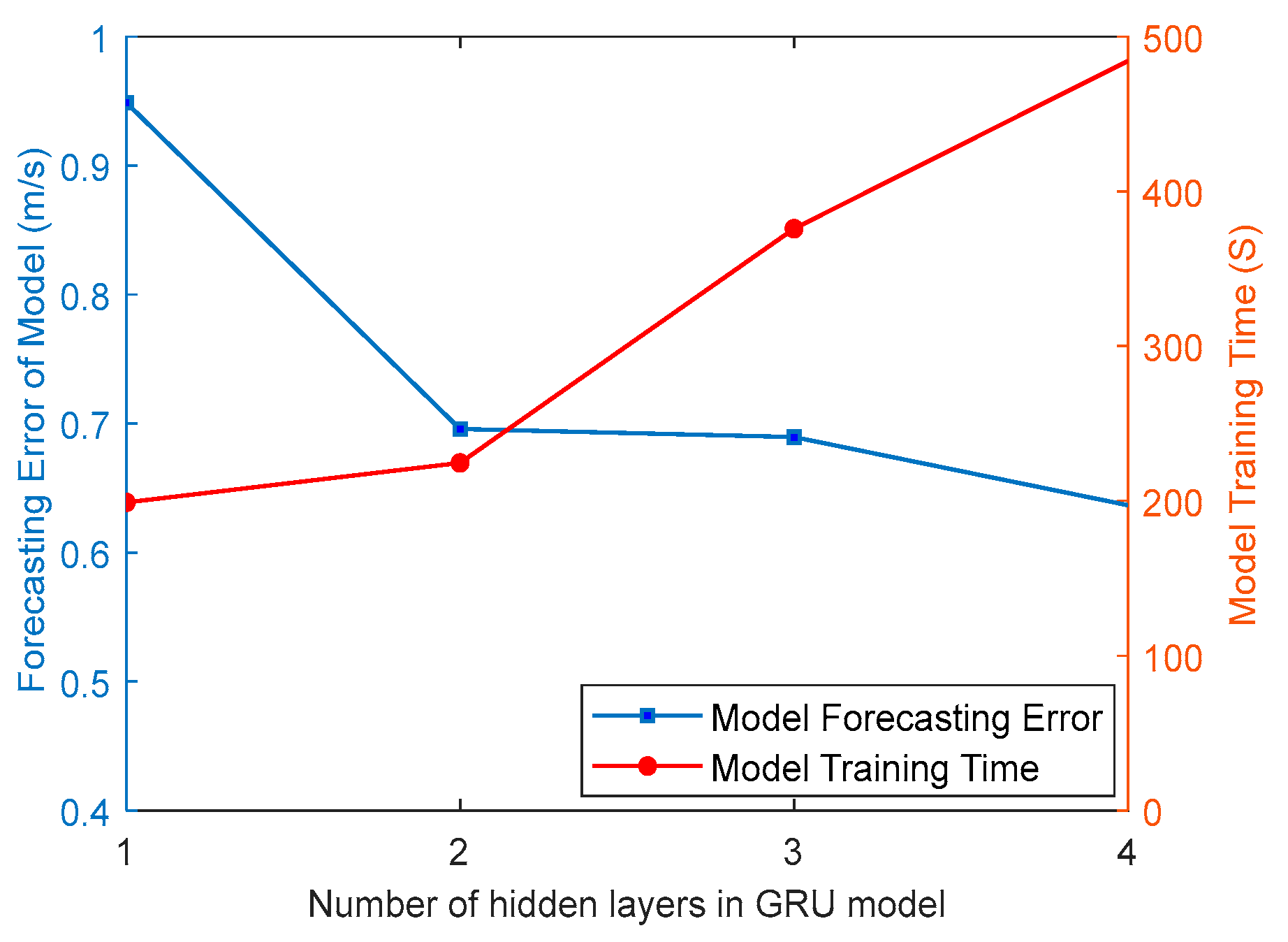
In theory, the greater the number of hidden layers the GRU model has, the higher the GRU model forecasting accuracy will be. However, the training time and computational memory requirements of the GRU model increase rapidly with the number of hidden layers. Additionally, a higher number of hidden layers may lead to issues such as overfitting and gradient vanishing. Therefore, selecting the appropriate number of hidden layers is critical for setting the hyperparameters of the GRU model.

Figure 3 shows the relationship between the model forecasting error (RMSE), model training time, and number of hidden layers (1, 2, 3, or 4) for the time series wind speed sequence in Dataset1. The solid blue line with squares represents the model forecasting error for different numbers of hidden layers, and the solid red line with dots represents the model training time. It can be observed that when the number of hidden layers is set to one, the GRU model has a relatively large forecasting error but requires less training time. As the number of hidden layers increases, the model forecasting accuracy improves; however, the training time also increases. When the number of hidden layers is two, the GRU model achieves the best balance between forecasting accuracy and training time.

(2)

Influence of the number of hidden layer neurons on the model forecasting performance

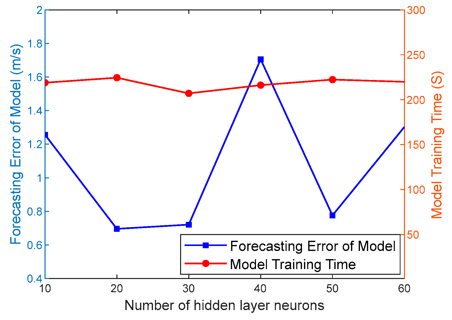
The number of hidden layer neurons also has a significant impact on the forecasting performance of the GRU model. When the number of hidden layer neurons is small, the GRU model is prone to underfitting; when there are too many neurons, the GRU model is prone to overfitting. Therefore, selecting a reasonable number of hidden layer neurons is also an important aspect of the hyperparameter settings in the GRU model. Figure 4 shows the correlations between the number of hidden layer neurons, model forecasting error, and training time. As shown in Figure 4, when the number of hidden layer neurons is 20, the forecasting accuracy and training time of the GRU model reach an optimal balance.

(3)

Impact of training epochs on the model forecasting performance

One training epoch represents a complete operation on the data in a neural network. The weight matrix in the GRU network must be updated every time the data are fully trained. Too few training epochs cannot accurately extract temporal features from the training data, resulting in underfitting of the GRU model. Excessive training epochs increase the training time of the GRU model. Therefore, determining a reasonable number of training epochs and accurately extracting temporal features from the data are important aspects to be considered in the hyperparameter setting of the GRU model.

As shown in Figure 5, when the number of training epochs for the GRU model is set to 70, the model achieves the lowest forecasting error, and the increase in training time is relatively minimal.

(4)

Impact of the learning rate and learning rate decay period on the model forecasting performance

The learning rate is a crucial hyperparameter that controls the learning progress of the GRU model. Setting a learning rate that is too high or too low can affect both the model training time and forecasting accuracy. Typically, a higher learning rate is used in the initial stages of model training to enhance the initial learning speed. After a certain number of training iterations, it is necessary to decrease the learning rate to improve the model forecasting accuracy.

Figure 6a illustrates the impact of the learning rate on the model forecasting accuracy and training time. As shown in Figure 6a, the GRU model achieves the best forecasting performance when the initial learning rate is set to 0.06.

Figure 6b shows the influence of the learning rate decay period on the model forecasting accuracy and training time. As shown in Figure 6b, the GRU model performs optimally when the learning rate decay period is set to 30.

Based on the information in Figure 3, Figure 4, Figure 5 and Figure 6, it is evident that setting the number of hidden layers, number of neurons in the hidden layer, number of training epochs, learning rate, and learning rate decay period appropriately can effectively improve the forecasting accuracy of the GRU model.

5.3. AOA Optimized Hyperparameters of the GRU Model

Based on the discussion in Section 5.2, it is clear that setting appropriate hyperparameters for the GRU model can improve the forecasting accuracy while reducing the model training time. However, in practical engineering applications, the training dataset is continually changing, and the GRU model hyperparameters must be adjusted accordingly. When the grid search method is used to adjust the GRU model, the hyperparameters are inefficient and may not meet the demands of real-world applications. Therefore, in this study, the AOA is utilized to optimize the GRU model hyperparameters, including the training data sequence length, number of hidden layer neurons, training epochs, initial learning rate, and learning rate decay period. The number of hidden layers in the GRU model is determined using a grid search method and remains constant throughout the optimization process. The construction process for the AOA-GRU model is illustrated in Figure 7.

The specific AOA optimization process for the hyperparameters of the GRU model is as follows.

Step 1: Construct an AOA candidate solution structure, X_i(x_i1, x_i2, x_i3, x_i4, x_i5), including the training data time series length, x_i1, number of hidden layer neurons, x_i2, training iterations, x_i3, initial learning rate, x_i4, and learning rate decay period, x_i5. Determine the range and number of candidate solutions.

Step 2: Based on the position coordinates X_i(x_i1, x_i2, x_i3, x_i4, x_i5) of each candidate solution, construct their respective GRU forecasting models and forecast the wind speed sequence.

Step 3: Calculate the forecasting error of each GRU model based on its forecasting results and use the forecasting error as the fitness value for each candidate solution of the AOA.

Step 4: Save the coordinates of the candidate solution with the best fitness value as X^*(x₁, x₂, x₃, x₄, x₅), representing the optimal model hyperparameters.

Step 5: Utilize the AOA to update the coordinates of each candidate solution X_i(x_i1, x_i2, x_i3, x_i4, x_i5) and rebuild each GRU model based on the updated coordinates to forecast the wind speed.

Step 6: Based on the forecasting results of the GRU model, recalculate the forecasting errors of each GRU model and determine the position coordinates X^*(x₁, x₂, x₃, x₄, x₅) of the candidate solution with the best fitness value, i.e., the optimal training data length and model hyperparameters.

Step 7: Check whether the termination condition is satisfied. If not, return to Step 5 and continue the process. If the termination condition is satisfied, proceed to Step 8.

Step 8: Build the final GRU forecasting model based on the coordinates of the global optimal candidate solution, X^*(x₁, x₂, x₃, x₄, x₅), to forecast the wind speed.

6. Construction and Verification of the VMD-AOA-GRU Model

6.1. Data Sources and Sample Set Partition

(1)

Data Sources

The wind speed data used in this study were derived from the Supervisory Control and Data Acquisition (SCADA) system of a wind farm located in the northwestern region of China that includes 134 wind turbines. The distribution of the wind turbines is shown in Figure 8. The relative coordinates of each turbine are shown in the figure, with the x- and y-axis units expressed in meters. The collection period for the wind speed data is 180 d, and the data time resolution is 10 min. Among them, the 58th and 123rd wind turbines (with red borders) are the research objects of this paper.

The ultra-short-term forecasting of wind speed mainly refers to the forecasting of one or several time steps in the future. In order to verify the high forecasting accuracy of the model proposed in this paper at different forecasting time scales, the ultra-short-term wind speeds of one time step, two time steps, and three time steps were forecasted, with each time step being 10 min.

(2)

Sample Set Partitioning

To validate the effectiveness of the proposed algorithm, the wind speed data from the 58th and 123rd wind turbines, located far apart, were selected for calculation and analysis. Additionally, to verify the forecasting performance of the proposed algorithm under different climatic conditions, four datasets from the 10th to the 19th day and from the 153rd to the 162nd day were chosen for model training and testing (two datasets per turbine). The datasets belonging to the 58th wind turbine were denoted as Dataset1 (from the 10th to the 19th day) and Dataset2 (from the 153rd to the 162nd day), while the datasets from the 123rd wind turbine were denoted as Dataset3 (from the 10th to the 19th day) and Dataset4 (from the 153rdto the 162nd day). Each dataset contained 1440 data points, with the first 1320 data points designated as the training dataset and the last 120 data points designated as the testing dataset.

6.2. VMD-AOA-GRU Model Construction

When forecasting the UTSWS, VMD was first used to decompose the time series wind speed data into different frequency time series data, thus effectively extracting the high-frequency data features from the wind speed data while removing noise and thereby enhancing the forecasting accuracy of the model. Subsequently, the constructed AOA-GRU model was used to train and test the temporal wind speed data at different frequencies. The implementation process for the entire VMD-AOA-GRU model is illustrated in Figure 9.

The specific implementation steps are as follows:

(1)

Utilize VMD to decompose the training and testing datasets and obtain K modal components of different frequencies.

(2)

Input each modal component derived from the decomposed training dataset into the AOA-GRU model separately and train the AOA-GRU model.

(3)

Input each modal component derived from the decomposed testing dataset into the trained AOA-GRU model to achieve ultra-short-term forecasting for each modal component.

(4)

Reconstruct the UTSWS based on the ultra-short-term forecasting results of each modal component of the testing dataset.

6.3. Verification of the VMD-AOA-GRU Model

6.3.1. Determination of the Number of VMD Modal Components

When the number of modal components in VMD is small, some important information in the original time series wind speed will be filtered out, reducing the forecasting accuracy of the VMD-AOA-GRU model. When the number of modal components is large, modal overlap can easily occur or additional noise may be generated. Therefore, the selection of an appropriate number of VMD modal components has become a key concern in VMD research and application. To determine the optimal number of temporal wind speed modal components, the number of temporal wind speed decomposed modal components was gradually increased in this study, and the Pearson correlation coefficient method was used to calculate the correlation coefficients between the decomposed modal components. The optimal number of VMD modal components can be determined by calculating their correlation coefficients.

Table 2. Central frequency distribution of the decomposed time series wind speed.

Number of Modes (K)	Central Frequency
2	0.1491 Hz	0.0004 Hz
3	0.3401 Hz	0.0776 Hz	0.0003 Hz
4	0.4367 Hz	0.1792 Hz	0.0551 Hz	0.0003 Hz
5	0.4494 Hz	0.2573 Hz	0.1002 Hz	0.0156 Hz	0.0002 Hz
6	0.3768 Hz	0.2106 Hz	0.1094 Hz	0.0529 Hz	0.0098 Hz	0.0001 Hz
7	0.3875 Hz	0.2525 Hz	0.1540 Hz	0.1007 Hz	0.0511 Hz	0.0092 Hz	0.0001 Hz
8	0.4255 Hz	0.3154 Hz	0.2231 Hz	0.1543 Hz	0.1033 Hz	0.0514 Hz	0.0088 Hz	0.0001 Hz

presents the center frequency distribution of the time series wind speed for Dataset1 after decomposition under different numbers of modal components. Table 2 demonstrates that as the number of modal components increases, the spacing between the center frequencies of each mode gradually decreases.

Table 3. Pearson correlation coefficients between adjacent modal components.

Number of Modal Components (K)	C12	C23	C34	C45	C56	C67	C78
2	0.015163
3	0.025336	0.04361
4	0.022502	0.061709	0.053189
5	0.035944	0.048752	0.069011	0.157038
6	0.040904	0.064714	0.109889	0.079833	0.144653
7	0.061023	0.072363	0.117903	0.132261	0.074168	0.14186
8	0.068861	0.085539	0.118399	0.116491	0.113842	0.066931	0.144964

presents the Pearson correlation coefficients between the various modal components of the original time series wind speed after decomposition under different numbers of modal components. The results reveal that when the number of modal components is two or three, the Pearson correlation coefficient between each modal component is low. However, because of the small number of modal components, important temporal wind speed information is easily lost. When the number of modal components is five, six, or greater, the Pearson correlation coefficient between some modal components is higher (bold font in Table 3), indicating the existence of overlap between these modal components. When the number of modal components is four, the Pearson correlation coefficient between each modal component is low, and the number of modal components is relatively small. Thus, it can be concluded that the most reasonable choice for the VMD calculation of the time series wind speed is four modal components. In the subsequent VMD calculation of the time series wind speed in this study, four modal components were used.

6.3.2. Training of VMD-AOA-GRU Model

It is necessary to train the VMD-AOA-GRU model to achieve ultra-short-term forecasting. When training the VMD-AOA-GRU model in this study, the training datasets used were the four training datasets introduced in Section 6.1 (Training Dataset 1, Training Dataset 2, Training Dataset 3, and Training Dataset 4). As described in Section 6.2 and Section 6.3.1, during the training of the VMD-AOA-GRU model using the training datasets, each group of training data needed to be decomposed into four modal components (resulting in 16 modal components from four datasets). Subsequently, the four VMD-AOA-GRU models were trained using the four decomposed modal components of each training dataset. In order to solve the problem of overfitting and bias during the model training process, the model was continuously trained 10 times, and the average hyperparameter value obtained from 10 times training was taken as the hyperparameter of the proposed model. The training process was executed on a laptop equipped with an Intel i7-6500U CPU running at a main frequency of 2.29 GHz and memory of 16 GB. The calculation software was MATLAB 2021a.

Table 4. Hyperparameter values of the GRU model optimized by AOA.

Sequence	Training Dataset 1				Training Dataset 2
Modal Components	1	2	3	4	1	2	3	4
Temporal Length of Training Data	21	17	9	47	14	11	10	20
Number of Neurons in Hidden Layers	28	50	21	50	50	30	50	44
Number of Training Epochs	91	81	75	100	100	34	71	89
Learning Rate	0.0478	0.0355	0.079	0.0572	0.0766	0.0581	0.0269	0.0574
Learning Rate Decay Period	15	30	9	16	10	25	29	30
MAE	3.46%	4.7%	4.32%	3.96%	7.54%	4.4%	3.23%	2.74%
RMSE	4.98%	6.59%	5.36%	4.82%	9.71%	5.81%	3.93%	3.35%
MAPE	0.53%	0.71%	0.85%	0.01%	0.62%	0.30%	0.21%	0.01%
Training Time	187.4 s	190.1 s	153.9 s	232.4 s	233.9 s	88.6 s	172.1 s	201.9 s
Sequence	Training Dataset 3				Training Dataset 4
Modal Components	1	2	3	4	1	2	3	4
Temporal Length of Training Data	9	10	9	56	9	16	11	20
Number of Neurons in Hidden Layers	39	44	16	24	30	33	34	48
Number of Training Epochs	67	83	62	96	58	96	35	80
Learning Rate	0.1	0.0391	0.1	0.0589	0.087	0.0544	0.0409	0.0564
Learning Rate Decay Period	30	30	30	30	26	25	30	17
MAE	4.51%	4.08%	2.12%	2.58%	3.66%	3.4%	3.14%	2.74%
RMSE	6.52%	5.53%	2.92%	3.13%	4.59%	4.41%	4.13%	3.47%
MAPE	1.60%	0.32%	0.12%	0.01%	2.51%	0.32%	0.15%	0.01%
Training Time	157.2 s	189.7 s	127.3 s	187.2 s	133 s	201.1 s	92.1 s	186.6 s

presents a detailed list of the hyperparameter values of the VMD-AOA-GRU model optimized by AOA during the one-step forecasting process. Table 4 reveals that (1) the hyperparameter values of the GRU model trained by different modal components obtained using the same training dataset are different, and (2) the hyperparameter values of the GRU model trained by different modal components obtained from different training datasets are different.

There are three reasons for this outcome.

(a)

The wind speed data features contained in the four modal components decomposed from the same training dataset differ. Therefore, after using the four modal components to train the AOA-GRU model, the hyperparameter values of the GRU model optimized by AOA are different.

(b)

Owing to the large distance between the 58th and 123rd wind turbines, there are certain differences in the time series wind speed data for these two turbines during the same time period, and the decomposed modal components also differ. After using these modal components to train the AOA-GRU model, the hyperparameter values of the GRU model optimized by AOA are different.

(c)

The time series wind speed data from the same wind turbine differ significantly during different time periods, and the decomposed modal components also exhibit significant differences. After training the AOA-GRU model using modal components, the hyperparameter values of the GRU model optimized by AOA are different.

From the above analysis, it can be observed that the hyperparameter values of the GRU model change with changes in the training dataset. Therefore, in the process of real-time forecasting of ultra-short-term wind speeds, it is necessary to use the AOA to optimize the hyperparameters of the GRU model in real time to obtain the optimal forecasting performance.

6.3.3. Forecasting Analysis of the VMD-AOA-GRU Model

To validate the performance of the proposed VMD-AOA-GRU model for ultra-short-term wind speed forecasting, the forecasting results of the GRU, VMD-GRU, AOA-GRU, and VMD-AOA-GRU models were compared at different forecasting time steps. The hyperparameter values of GRU and VMD-GRU were adjusted using the grid search method, which ensured that these models were under fair comparison conditions during the comparison process. The training dataset of these models was derived from the training data described in Section 6.1, and the forecasting results of the four testing datasets (Testing Dataset1, Testing Dataset2, Testing Dataset3, and Testing Dataset4) are shown in Figure 10.

In Figure 10, the black solid line represents the actual observed wind speed, the blue solid line represents the forecasting of the GRU model, the yellow solid line represents the forecasting of the VMD-GRU model, the green solid line represents the forecasting of the AOA-GRU model, and the red solid line represents the forecasting of the VMD-AOA-GRU model.

Based on the forecasting results in Figure 10, the following conclusions can be drawn.

(1)

Under different forecasting time steps, all four forecasting models can accurately reflect the trend of actual wind speed changes, confirming that the GRU model and its hybrid model perform well in time series wind speed forecasting.

(2)

The wind speed inflection point in Figure 10 reveals that the forecasting results of the GRU and AOA-GRU models lag behind those of the VMD-GRU and VMD-AOA-GRU models. This is because the VMD algorithm can effectively extract high-frequency component features (corresponding to the rapidly changing part of the wind speed) from the wind speed sequence, and these high-frequency component features are used as a component of the input data of the forecasting model, enabling the VMD-GRU and VMD-AOA-GRU models to accurately forecast the sudden changes in the actual wind speed.

Table 5. Forecasting error values at different forecasting time steps.

	Time Steps	1			2			3
	Error Type	MAE	RMSE	MAPE	MAE	RMSE	MAPE	MAE	RMSE	MAPE
Testing Dataset 1	GRU	0.5499	0.7527	0.0734	0.7272	0.9096	0.0964	0.7524	0.9413	0.0994
	VMD-GRU	0.4159	0.5091	0.0576	0.5143	0.6375	0.0710	0.6018	0.7176	0.0846
	AOA-GRU	0.5178	0.7378	0.0696	0.6743	0.8652	0.0912	0.7420	0.9236	0.1007
	VMD-AOA-GRU	0.2280	0.2990	0.0292	0.2536	0.3382	0.0323	0.2704	0.3585	0.0349
Testing Dataset 2	GRU	0.7005	0.9290	0.1615	0.8503	1.0866	0.2025	0.9865	1.2427	0.2413
	VMD-GRU	0.3967	0.5232	0.0927	0.5400	0.6781	0.1274	0.5542	0.6989	0.1354
	AOA-GRU	0.5259	0.7174	0.1227	0.7793	1.0050	0.1807	0.9585	1.2020	0.2235
	VMD-AOA-GRU	0.2463	0.3001	0.0615	0.2727	0.3286	0.0641	0.3411	0.4422	0.0843
Testing Dataset 3	GRU	0.5426	0.7111	0.0728	0.7227	0.8794	0.0982	0.7178	0.8949	0.0977
	VMD-GRU	0.3390	0.4373	0.0483	0.3697	0.4769	0.0508	0.4685	0.6097	0.0660
	AOA-GRU	0.4937	0.6592	0.0659	0.6291	0.8042	0.0838	0.6862	0.8508	0.0918
	VMD-AOA-GRU	0.1988	0.2576	0.0263	0.2027	0.2729	0.0269	0.2363	0.2923	0.0301
Testing Dataset 4	GRU	0.6143	0.7849	0.2029	0.6785	0.8854	0.2218	0.8397	1.0956	0.2713
	VMD-GRU	0.3970	0.4965	0.1346	0.4283	0.5355	0.1489	0.5287	0.6590	0.1756
	AOA-GRU	0.4425	0.5597	0.1387	0.6373	0.8183	0.2145	0.7011	0.9456	0.2094
	VMD-AOA-GRU	0.2170	0.2779	0.0701	0.2608	0.3351	0.0855	0.3102	0.3908	0.1054

presents the forecasting error values for the GRU, VMD-GRU, AOA-GRU, and VMD-AOA-GRU models at different forecasting time steps. The following conclusions are drawn based on the results in Table 5:

(1)

The VMD-GRU model outperforms the GRU model in terms of forecasting accuracy, and the VMD-AOA-GRU model exhibits a higher forecasting accuracy than the AOA-GRU model. This demonstrates that the VMD algorithm effectively captures the high-frequency components of the wind speed data, thereby enhancing the forecasting accuracy of the forecasting models.

(2)

The AOA-GRU model outperforms the GRU model in terms of forecasting accuracy, and the VMD-AOA-GRU model outperforms the VMD-GRU model in terms of forecasting accuracy. This indicates that utilizing the AOA to optimize the hyperparameters of the GRU model can effectively improve its forecasting accuracy.

(3)

For the different forecasting models, as the forecasting time step increases, the forecasting error also increases.

7. Comparison of Different Forecasting Models

To further demonstrate the superiority of the proposed VMD-AOA-GRU forecasting model, a comparative analysis was conducted for the multiple-step forecasting of various models. The compared models included the LSTM, GRU, PSO-BP, PSO-ELM, PSO-LSSVM, VMD-GRU, VMD-LSTM, VMD-PSO-BP, VMD-PSO-ELM, VMD-PSO-LSSVM, and VMD-AOA-GRU models. In order to ensure that these models were under fair comparison conditions during the comparison process, except for the VMD-AOA-GRU model, the hyperparameters of all other models were optimized using the grid search method. The forecasting results for these models are shown in Figure 11. The training and testing datasets used for the comparative analysis were consistent with those presented in Section 6.1.

In Figure 11, the black solid line represents the observed wind speed, the blue dashed line represents the forecasting of the LSTM model, the purple dashed line represents the forecasting of the GRU model, the orange dashed line represents the forecasting of the PSO-BP model, the green dashed line represents the forecasting of the PSO-ELM model, the cyan dashed line represents the forecasting of the PSO-LSSVM model, and the red solid line represents the forecasting of the VMD-AOA-GRU model. Based on the observations and analysis shown in Figure 11, the following conclusions can be drawn.

(1)

All of the machine learning models accurately capture the trends of the actual wind speed, demonstrating that the use of machine learning models for ultra-short-term wind speed forecasting is feasible.

(2)

At the wind speed inflection points, the VMD-AOA-GRU, VMD-LSTM, VMD-GRU, VMD-PSO-BP, VMD-PSO-ELM, and VMD-PSO-LSSVM models accurately forecast the positions of the inflection points (the highest accuracy in single-step forecasting). In contrast, the other models exhibit a lag in forecasting the positions of the inflection points compared with the actual wind speed. This further validates that the VMD algorithm can accurately extract the high-frequency components of the time series wind speed, thereby enhancing the accuracy of wind-speed forecasting.

(3)

Among the forecasting models, the VMD-AOA-GRU model shows the closest similarity to the distribution characteristics of the actual time series wind speed. This demonstrates that the forecasting performance of the VMD-AOA-GRU model is superior to that of the other models.

Table 6. Wind speed forecasting errors of different models.

	Time Step	1			2			3
	Error Type	MAE	RMSE	MAPE	MAE	RMSE	MAPE	MAE	RMSE	MAPE
Testing Dataset 1	LSTM	0.7122	0.8927	0.0948	0.7605	0.9483	0.1004	0.8092	1.0211	0.1049
	GRU	0.5499	0.7527	0.0734	0.7272	0.9096	0.0964	0.7524	0.9413	0.0994
	PSO-BP	0.5722	0.8016	0.0760	0.7276	0.9305	0.0971	0.7565	1.0682	0.1002
	PSO-ELM	0.2937	0.3873	0.0399	0.4859	0.6034	0.0654	0.5159	0.6478	0.0698
	PSO-LSSVM	0.5241	0.7260	0.0716	0.6662	0.8312	0.0919	0.7286	0.8855	0.0995
	VMD-LSTM	0.4140	0.5131	0.0593	0.4148	0.5472	0.0545	0.4637	0.6218	0.0596
	VMD-GRU	0.4159	0.5091	0.0576	0.5143	0.6375	0.0710	0.6018	0.7176	0.0846
	VMD-PSO-BP	0.2306	0.2987	0.0292	0.2896	0.3994	0.0367	0.3467	0.4775	0.0444
	VMD-PSO-ELM	0.2371	0.3172	0.0302	0.4253	0.5602	0.0560	0.4832	0.6103	0.0638
	VMD-PSO-LSSVM	0.2295	0.3045	0.0293	0.2888	0.3955	0.0367	0.3162	0.4365	0.0406
	VMD-AOA-GRU	0.2280	0.2990	0.0292	0.2536	0.3382	0.0323	0.2704	0.3585	0.0349
Testing Dataset 2	LSTM	0.7528	1.0541	0.1643	0.8739	1.1703	0.1995	1.0092	1.3030	0.2428
	GRU	0.7005	0.9290	0.1615	0.8503	1.0866	0.2025	0.9865	1.2427	0.2413
	PSO-BP	0.5447	0.7329	0.1265	0.7984	1.0600	0.1791	0.9295	1.2103	0.2099
	PSO-ELM	0.4124	0.5301	0.1029	0.5670	0.7277	0.1419	0.6451	0.8573	0.1566
	PSO-LSSVM	0.6130	0.8520	0.1380	0.7448	0.9983	0.1696	0.9032	1.2067	0.2007
	VMD-LSTM	0.4073	0.5381	0.0953	0.4659	0.6060	0.1026	0.5551	0.7177	0.1266
	VMD-GRU	0.3967	0.5232	0.0927	0.5400	0.6781	0.1274	0.5542	0.6989	0.1354
	VMD-PSO-BP	0.2496	0.3046	0.0632	0.3523	0.3535	0.0649	0.4273	0.5705	0.1002
	VMD-PSO-ELM	0.2564	0.3070	0.0643	0.2618	0.4604	0.0820	0.4124	0.5346	0.0971
	VMD-PSO-LSSVM	0.2474	0.3066	0.0622	0.2848	0.3730	0.0677	0.4589	0.6011	0.1071
	VMD-AOA-GRU	0.2463	0.3001	0.0615	0.2727	0.3286	0.0641	0.3411	0.4422	0.0843
Testing Dataset 3	LSTM	0.6011	0.7619	0.0798	0.7163	0.8916	0.0954	0.8098	0.9865	0.1089
	GRU	0.5426	0.7111	0.0728	0.7227	0.8794	0.0982	0.7178	0.8949	0.0977
	PSO-BP	0.4963	0.6558	0.0648	0.6969	0.8854	0.0921	0.7414	0.9364	0.0981
	PSO-ELM	0.3469	0.4394	0.0462	0.4447	0.5677	0.0597	0.5260	0.6446	0.0713
	PSO-LSSVM	0.6398	0.7872	0.0854	0.7180	0.8766	0.0957	0.7375	0.8947	0.0981
	VMD-LSTM	0.2927	0.3846	0.0399	0.4904	0.5983	0.0691	0.4918	0.6181	0.0696
	VMD-GRU	0.3390	0.4373	0.0483	0.3697	0.4769	0.0508	0.4685	0.6097	0.0660
	VMD-PSO-BP	0.2078	0.2755	0.0277	0.2502	0.2790	0.0337	0.2645	0.3690	0.0350
	VMD-PSO-ELM	0.2006	0.2716	0.0265	0.2085	0.3570	0.0277	0.2253	0.3981	0.0405
	VMD-PSO-LSSVM	0.2031	0.2690	0.0269	0.2040	0.2835	0.0270	0.2978	0.3371	0.0311
	VMD-AOA-GRU	0.1988	0.2576	0.0263	0.2027	0.2729	0.0269	0.2363	0.2923	0.0301
Testing Dataset 4	LSTM	0.7196	0.9250	0.2394	0.8377	1.0775	0.2821	0.8782	1.1983	0.2640
	GRU	0.6143	0.7849	0.2029	0.6785	0.8854	0.2218	0.8397	1.0956	0.2713
	PSO-BP	0.4324	0.5544	0.1331	0.6957	0.9454	0.2054	0.7131	0.9583	0.2135
	PSO-ELM	0.3143	0.4076	0.1008	0.4435	0.5777	0.1375	0.5032	0.6291	0.1586
	PSO-LSSVM	0.4349	0.5586	0.1345	0.6184	0.8034	0.1848	0.7263	0.9627	0.2155
	VMD-LSTM	0.4238	0.5176	0.1448	0.4586	0.5561	0.1585	0.5844	0.7049	0.2096
	VMD-GRU	0.3970	0.4965	0.1346	0.4283	0.5355	0.1489	0.5287	0.6590	0.1756
	VMD-PSO-BP	0.2177	0.2902	0.0730	0.3526	0.3358	0.1138	0.3906	0.5082	0.1267
	VMD-PSO-ELM	0.2239	0.2860	0.0728	0.2620	0.4415	0.0872	0.4021	0.5043	0.1239
	VMD-PSO-LSSVM	0.2250	0.2785	0.0704	0.2778	0.3551	0.0904	0.3554	0.4476	0.1145
	VMD-AOA-GRU	0.2170	0.2779	0.0701	0.2608	0.3351	0.0855	0.3102	0.3908	0.1054

lists the forecasting errors of each forecasting model under the four testing wind speed sequences at one, two, and three steps. The following conclusions are drawn based on the results in Table 6:

(1)

The forecasting accuracy of the hybrid VMD models is higher than that of the non-hybrid VMD models, indicating that deep mining of high-frequency features in the time series wind speed through VMD can effectively improve the forecasting accuracy of the forecasting model.

(2)

The forecasting accuracy of the LSTM and GRU models is lower than that of some machine learning models, indicating that although the LSTM and GRU models have the theoretical potential to achieve high forecasting accuracy by mining temporal correlations in the data, their forecasting accuracy is affected by improper hyperparameter settings.

(3)

The forecasting accuracy of the VMD-AOA-GRU model is higher than that of all other models, demonstrating that optimizing the hyperparameters of the GRU model through AOA effectively enhances the forecasting accuracy of the GRU model.

(4)

As the forecasting time step increases, the forecasting accuracy of all models gradually decreases, which aligns with the inherent characteristics of forecasting models.

8. Conclusions

This study proposes an ultrashort-term forecasting model for time series wind speeds based on VMD-AOA-GRU. The model first uses VMD to decompose the time series wind speed data into different frequency modal components, effectively extracting high-frequency wind speed features. Then, the AOA is employed to optimize the hyperparameters of the GRU model to construct a high-accuracy AOA-GRU forecasting model. The time series modal components decomposed by VMD are then employed to train and test the AOA-GRU model, achieving multi-step forecasting of ultra-short-term time series wind speeds. The forecasting results for the GRU, VMD-GRU, VMD-AOA-GRU, LSTM, PSO-BP, PSO-ELM, PSO-LSSVM, VMD-LSTM, VMD-PSO-BP, VMD-PSO-ELM, and VMD-PSO-LSSVM models were compared, and the results are as follows:

(1)

The forecasting accuracies of the hybrid VMD models (VMD-AOA-GRU, VMD-LSTM, VMD-PSO-BP, VMD-PSO-ELM, and VMD-PSO-LSSVM) are higher than those of the non-hybrid VMD models (GRU, LSTM, PSO-BP, PSO-ELM, and PSO-LSSVM), indicating that the VMD can deeply explore high-frequency components in time series wind speed, particularly the high-frequency features at inflection points, effectively improving the accuracy of the forecasted time series wind speed.

(2)

Although the LSTM and GRU deep learning models can capture the temporal correlations in time series wind speeds, their forecasting accuracy may be lower than that of some commonly used machine learning models (PSO-BP, PSO-ELM, and PSO-LSSVM) when their hyperparameter settings are improper. This indicates that a reasonable setting of hyperparameters for deep learning models significantly affects the forecasting accuracy.

(3)

The forecasting accuracy of the GRU model can be effectively improved by using the AOA to optimize the hyperparameters of the GRU model. The calculation results show that the forecasting accuracy of the VMD-AOA-GRU model constructed in this study is higher than that of the other models.

(4)

As the forecasting time step increases, the forecasting accuracy of the model gradually decreases.

The study results in this paper can be widely used for the optimization control of wind turbines, thereby improving the operational efficiency of wind turbines and reducing their fatigue losses. However, during the research process, this paper did not consider the accuracy of wind direction forecasting, a topic that will need to be a focus of subsequent research.

References

1. IRENA. Renewable Capacity Statistics 2023. Available online: https://www.irena.org/Publications/2023/Mar/Renewable-capacity-statistics-2023 (accessed on 29 September 2023).
2. GWEC. Global Wind Report 2023. Available online: https://gwec.net/globalwindreport2023/ (accessed on 29 September 2023).
3. Saini, V.K.; Kumar, R.; Al-Sumaiti, A.S.; Sujil, A.; Heydarian-Forushani, E. Learning Based Short Term Wind Speed Forecasting Models for Smart Grid Applications: An Extensive Review and Case Study. Electr. Power Syst. Study 2023, 222, 109502. [Google Scholar] [CrossRef]
4. Wang, Y.; Zou, R.; Liu, F.; Zhang, L.; Liu, Q. A Review of Wind Speed and Wind Power Forecasting with Deep Neural Networks. Appl. Energy 2021, 304, 117766. [Google Scholar] [CrossRef]
5. Shahram, H.; Liu, X.L.; Lin, Z.; Saeid, L. A Critical Review of Wind Power Forecasting Methods-Past, Present and Future. Energies 2020, 13, 3764. [Google Scholar]
6. Wang, J.; Song, Y.; Liu, F.; Hou, R. Analysis and Application of Forecasting Models in Wind Power Integration: A Review of Multi-Step-Ahead Wind Speed Forecasting Models. Renew. Sustain. Energy Rev. 2016, 60, 960–981. [Google Scholar] [CrossRef]
7. Han, Y.; Mi, L.; Shen, L.; Cai, C.; Liu, Y.; Li, K.; Xu, G. A Short-Term Wind Speed Prediction Method Utilizing Novel Hybrid Deep Learning Algorithms to Correct Numerical Weather Forecasting. Appl. Energy 2022, 312, 118777. [Google Scholar] [CrossRef]
8. Lydia, M.; Kumar, S.S.; Selvakumar, A.I.; Kumar, G.E.P. Linear and Non-Linear Autoregressive Models for Short-Term Wind Speed Forecasting. Energy Convers. Manag. 2016, 112, 115–124. [Google Scholar] [CrossRef]
9. Srihari, P.; Kiran, T.; Vishalteja, K. A Hybrid VMD Based Contextual Feature Representation Approach for Wind Speed Forecasting. Renew. Energy 2023, 219, 119391. [Google Scholar]
10. Zhang, Y.; Zhao, Y.; Kong, C.; Chen, B. A New Prediction Method Based on VMD-PRBF-ARMA-E Model Considering Wind Speed Characteristic. Energy Convers. Manag. 2020, 203, 112254. [Google Scholar] [CrossRef]
11. Zhu, K.; Mu, L.; Yu, R.; Xia, X.; Tu, H. Probabilistic Modelling of Surface Drift Prediction in Marine Disasters Based on the NN-GA and ARMA Model. Ocean Eng. 2023, 281, 114804. [Google Scholar] [CrossRef]
12. Zhu, Y.; Xie, S.; Xie, Y.; Chen, X. Temperature Prediction of Aluminum Reduction Cell Based on Integration of Dual Attention LSTM for Non-Stationary Sub-Sequence and ARMA for Stationary Sub-Sequences. Control Eng. Pract. 2023, 138, 105567. [Google Scholar] [CrossRef]
13. Aasim Singh, S.N.; Mohapatra, A. Repeated Wavelet Transform Based ARIMA Model for Very Short-Term Wind Speed Forecasting. Renew. Energy 2019, 136, 758–768. [Google Scholar] [CrossRef]
14. Liu, X.L.; Lin, Z.; Feng, Z.M. Short-term Offshore Wind Speed Forecast by Seasonal ARIMA-A Comparison against GRU and LSTM. Energy 2021, 227, 120492. [Google Scholar] [CrossRef]
15. Akshita, G.; Arun, K. Two-Step Daily Reservoir Inflow Prediction Using ARIMA-Machine Learning and Ensemble Models. J. Hydro-Environ. Res. 2022, 45, 39–52. [Google Scholar]
16. Hu, Y.H.; Guo, Y.S.; Fu, R. A Novel Wind Speed Forecasting Combined Model Using Variational Mode Decomposition, Sparse Auto-Encoder and Optimized Fuzzy Cognitive Mapping Network. Energy 2023, 278 Pt A, 127926. [Google Scholar] [CrossRef]
17. Li, M.; Yang, Y.; He, Z.; Guo, X.; Zhang, R.; Huang, B. A Wind Speed Forecasting Model Based on Multi-objective Algorithm and Interpretability Learning. Energy 2023, 269, 126778. [Google Scholar] [CrossRef]
18. Parmaksiz, H.; Yuzgec, U.; Dokur, E.; Erdogan, N. Mutation Based Improved Dragonfly Optimization Algorithm for a Neuro-fuzzy System in Short Term Wind Speed Forecasting. Knowl.-Based Syst. 2023, 268, 110472. [Google Scholar] [CrossRef]
19. Dokur, E.; Erdogan, N.; Salari, M.E.; Karakuzu, C.; Murphy, J. Offshore Wind Speed Short-Term Forecasting Based on a Hybrid Method: Swarm Decomposition and Meta-Extreme Learning Machine. Energy 2022, 248, 123595. [Google Scholar] [CrossRef]
20. Yang, Y.; Zhou, H.; Wu, J.; Ding, Z.; Wang, Y.-G. Robustified Extreme Learning Machine Regression with Applications in Outlier-Blended Wind-Speed Forecasting. Appl. Soft Comput. 2022, 122, 108814. [Google Scholar] [CrossRef]
21. Sun, S.; Wang, Y.; Meng, Y.; Wang, C.; Zhu, X. Multi-Step Wind Speed Forecasting Model Using a Compound Forecasting Architecture and an Improved QPSO-Based Synchronous Optimization. Energy Rep. 2022, 8, 9899–9918. [Google Scholar] [CrossRef]
22. He, Y.; Wang, Y.; Wang, S.; Yao, X. A Cooperative Ensemble Method for Multistep Wind Speed Probabilistic Forecasting. Chaos Solitons Fractals 2022, 162, 112416. [Google Scholar] [CrossRef]
23. Yang, W.; Hao, M.; Hao, Y. Innovative Ensemble System Based on Mixed Frequency Modeling for Wind Speed Point and Interval Forecasting. Inf. Sci. 2023, 622, 560–586. [Google Scholar] [CrossRef]
24. Dong, Y.; Li, J.; Liu, Z.; Niu, X.; Wang, J. Ensemble Wind Speed Forecasting System Based on Optimal Model Adaptive Selection Strategy: Case Study in China. Sustain. Energy Technol. Assess. 2022, 53 Pt B, 102535. [Google Scholar] [CrossRef]
25. Hao, Y.; Yang, W.D.; Yin, K.D. Novel Wind Speed Forecasting Model Based on a Deep Learning Combined Strategy in Urban Energy Systems. Expert Syst. Appl. 2023, 219, 119636. [Google Scholar] [CrossRef]
26. Wang, Y.; Xu, H.; Song, M.; Zhang, F.; Li, Y.; Zhou, S.; Zhang, L. A Convolutional Transformer-based Truncated Gaussian Density Network with Data Denoising for Wind Speed Forecasting. Appl. Energy 2023, 333, 120601. [Google Scholar] [CrossRef]
27. Lv, M.; Li, J.; Niu, X.; Wang, J. Novel Deterministic and Probabilistic Combined System Based on Deep Learning and Self-improved Optimization Algorithm for Wind Speed Forecasting. Sustain. Energy Technol. Assess. 2022, 52 Pt B, 102186. [Google Scholar] [CrossRef]
28. Gao, Z.; Li, Z.; Xu, L.; Yu, J. Dynamic Adaptive Spatio-temporal Graph Neural Network for Multi-node Offshore Wind Speed Forecasting. Appl. Soft Comput. 2023, 141, 110294. [Google Scholar] [CrossRef]
29. Sibtain, M.; Bashir, H.; Nawaz, M.; Hameed, S.; Azam, M.I.; Li, X.; Abbas, T.; Saleem, S. A Multivariate Ultra-Short-Term Wind Speed Forecasting Model by Employing Multistage Signal Decomposition Approaches and a Deep Learning Network. Energy Convers. Manag. 2022, 263, 115703. [Google Scholar] [CrossRef]
30. Nascimento, E.G.S.; Talison, A.C.; Davidson, M.M. A Transformer-Based Deep Neural Network with Wavelet Transform for Forecasting Wind Speed and Sind Energy. Energy 2023, 278, 127678. [Google Scholar] [CrossRef]
31. Bentsen, L.Ø.; Warakagoda, N.D.; Stenbro, R.; Engelstad, P. Spatio-Temporal Wind Speed Forecasting Using Graph Networks and Novel Transformer Architectures. Appl. Energy 2023, 333, 120565. [Google Scholar] [CrossRef]
32. Bala, S.B.; Kiran, T.; Vishalterja, K. Hybrid Wind Speed Forecasting Using ICEEMDAN and Transformer Model with Novel Loss Function. Energy 2023, 265, 126383. [Google Scholar]
33. Wu, H.; Meng, K.; Fan, D.; Zhang, Z.; Liu, Q. Multistep Short-Term Wind Speed Forecasting Using Transformer. Energy 2022, 261 Pt A, 125231. [Google Scholar] [CrossRef]
34. Liu, G.; Wang, Y.; Qin, H.; Shen, K.; Liu, S.; Shen, Q.; Qu, Y.; Zhou, J. Probabilistic Spatiotemporal Forecasting of Wind Speed Based on Multi-Network Deep Ensembles Method. Renew. Energy 2023, 209, 231–247. [Google Scholar] [CrossRef]
35. Lv, S.X.; Wang, L. Multivariate Wind Speed Forecasting Based on Multi-Objective Feature Selection Approach and Hybrid Deep Learning Model. Energy 2023, 263 Pt E, 126100. [Google Scholar] [CrossRef]
36. Zheng, L.; Lu, W.S.; Zhou, Q.Y. Weather Image-Based Short-Term Dense Wind Speed Forecast with a ConvLSTM-LSTM Deep Learning Model. Build. Environ. 2023, 239, 110446. [Google Scholar] [CrossRef]
37. Zhang, Y.M.; Wang, H. Multi-Head Attention-Based Probabilistic CNN-BiLSTM for Day-Ahead Wind Speed Forecasting. Energy 2023, 278 Pt A, 127865. [Google Scholar] [CrossRef]
38. Wang, J.Z.; An, Y.N.; Lu, H.Y. A Novel Combined Forecasting Model Based on Neural Networks, Deep Learning Approaches, and Multi-Objective Optimization for Short-Term Wind Speed Forecasting. Energy 2022, 251, 123960. [Google Scholar] [CrossRef]
39. Dragomiretskiy, K.; Zosso, D. Variational Mode Decomposition. IEEE Trans. Signal Process. 2014, 62, 531–544. [Google Scholar] [CrossRef]
40. Abualigah, L.; Diabat, A.; Mirjalili, S.; Abd Elaziz, M.; Gandomi, A.H. The Arithmetic Optimization Algorithm. Comput. Methods Appl. Mech. Eng. 2021, 376, 113609. [Google Scholar] [CrossRef]
41. Cho, K.; van Merriënboer, B.; Gulcehre, C.; Bahdanau, D.; Bougares, F.; Schwenk, H.; Bengio, Y. Learning Phrase Representations Using RNN Encoder-Decoder for Statistical Machine Translation. arXiv 2014, arXiv:1406.1078. [Google Scholar] [CrossRef]
42. Bahdanau, D.; Cho, K.; Bengio, Y. Neural Machine Translation by Jointly Learning to Align and Translate. arXiv 2014, arXiv:1409.0473. [Google Scholar] [CrossRef]
Figure 1. Principle of time series wind speed forecasting.
Processes 11 03247 g001
Figure 2. Internal structure of the GRU.
Processes 11 03247 g002
Figure 3. Relationships among the number of hidden layers, forecasting error, and training time.
Processes 11 03247 g003
Figure 4. Relationship among the number of hidden layer neurons, forecasting error, and training time.
Processes 11 03247 g004
Figure 5. Relationship among the number of training epochs, forecasting error, and training time.
Processes 11 03247 g005
Figure 6. Relationship among the learning rate, learning rate decay period, forecasting error, and training time. (a) Impact of the learning rate on the model forecasting performance. (b) Impact of the learning rate decay period on the model forecasting performance.
Processes 11 03247 g006
Figure 7. Construction process for the AOA-GRU model.
Processes 11 03247 g007
Figure 8. Wind turbine location distribution of wind farm.
Processes 11 03247 g008
Figure 9. Implementation process for the VMD-AOA-GRU model.
Processes 11 03247 g009
Figure 10. Multi-step forecasting results for the GRU model and its improved model.
Processes 11 03247 g010aProcesses 11 03247 g010b
Figure 11. Wind speed forecasting accuracy of different forecasting models.
Processes 11 03247 g011