Abstract
In mineral metallurgy, the flashing unit is key to returning the slurry to atmospheric conditions. Its primary function is to achieve pressure letdown, and during the process, shock waves are generated to maximize energy dissipation. Investigating the location and expansion of shock waves is the focal point of this study due to their importance in flashing unit design. A CFD model coupled with a homogeneous relaxation model (HRM) was used to simulate the flashing process of mineral slurry. The flow behavior, including velocity, pressure, and the shape and location of the shock waves, were obtained using simulation under different unit design and operating parameters. These results would provide valuable insights into the design of flashing units and guidance for the safe operation and maintenance of devices.
1. Introduction
With an increasing demand for non-ferrous materials, a greater number of studies are being conducted on the extraction and production of minerals. Several types of metallurgical processing are reviewed in many papers, mainly pyrometallurgical and hydrometallurgical [1,2,3,4]. Within these methodologies, a pivotal stage is leaching, which plays a crucial role in the extraction of metals. Mineral leaching often requires high temperatures and pressures. After the process, the resulting mineral slurry must be cooled to normal temperatures and pressures for further processing, such as separating and drying [5].
The flashing unit, located behind the autoclave, is the key equipment for returning the resulting mineral slurry to atmospheric conditions and minimizing solid residue, thus preparing it for further processing. The flashing unit plays a crucial role in the two-phase separation process, enabling rapid boiling and the vaporization of the liquid. To achieve this, the flashing valve is utilized to depressurize and vaporize the hot slurry, while the flashing tank provides sufficient space for effective vaporization and liquid separation. As a result, the design of the flashing unit, consisting of the flashing valve and tank, has a significant impact on maintenance costs and processing efficiency. Higher processing efficiency implies greater nozzle exit velocity, which increases the risk of damaging the bottom of the tank through collisions. In mineral metallurgy, it is common to incorporate multiple flashing tanks, typically exceeding three in number. Gradual pressure reduction offers notable advantages regarding safety performance and energy efficiency, leading to improved operational outcomes. The control methodology employed in the flashing system is commonly achieved by effectively managing two key aspects: (1) the operation conditions encompassing critical parameters such as inlet/upstream pressure, temperature, backpressure, and liquid level, and (2) the structure of the flashing valve and tank, including the angle of expansion of the nozzle and the opening of the valve, etc. The typical structures of the nozzles include the blast tube and the choke tube [6]. Their design aims to reduce the exit slurry velocity by controlling the position and expansion of the shock waves, ensuring the stability and safe operation of the device. Therefore, accurately capturing the position and expansion of the shock waves in the flashing slurry system is crucial for the design of this device.
Under industrial conditions, the complex multiphase behavior of high temperatures, high pressures, and the interactions between gas, liquids, and solids results in extremely complex phenomena of a highly compressible flow, violent phase change, and heat transfer. As a result, predicting and controlling the flow patterns associated with these phenomena present challenges [7]. Presently, there is a notable scarcity of visualization studies examining flashing slurry flow [8]. Therefore, numerical simulation has become useful for studying flashing slurry flow [8]. Smith et al. [6] and Fluerenbrock et al. [9] simulated the system using a mixture model coupled with a thermodynamic equilibrium assumption, focusing on the phase changes and shock waves, which are critical issues in this system. The simulations [6,9] showed that the mixture model captured the essential physics of the system. Employing this method offered valuable guidance for subsequent simulations of the system.
The phase change model plays an important role in the modeling of slurry flashing, as phase change is a critical feature of this process. The phase change is influenced by both temperature and pressure, with the abrupt pressure drop being the more crucial factor during slurry flashing. On the other hand, the sudden pressure change causes slurry flashing to deviate from thermodynamic equilibrium. Consequently, assuming thermodynamic equilibrium would lead to deviations between model predictions and the actual process. Due to this, the phase change models used in flashing simulations must take into account the non-equilibrium thermodynamic effects during rapid pressure-driven phase changes. Several phase change models focus on sudden pressure changes, including the Hertz–Knudsen equation [10], the Zwart–Gerber–Belamri model [11], the homogeneous relation model (HRM) [12], etc. In addition to the HRM model, the estimation of the density and distribution of activated nucleation sites is required for the derivation of the mass transfer rate in other phase change models [13]. However, the role of solid particles as nucleation sites has not been investigated [8]. In the HRM model, non-equilibrium states between liquids and gases are described using the relationship between the evaporation rate, the deviation in vapor quality or mass fraction X from equilibrium, and the relaxation time Θ. It explains the tendency of liquids to become metastable before boiling, a result of a finite rate of heat and the mass transfer between phases. A detailed explanation of the relaxation time can be found in the work of Zapolski et al. [14], in which empirical parameters were employed to fit the relaxation time in flashing water flow experiments. The HRM has been proposed as suitable for the prediction of flashing flow. It employs an empirical time scale correlation for thermal non-equilibrium effects between the two phases [15]. Although the HRM is a semi-empirical model, numerous studies have demonstrated its applicability to flashing systems [16,17,18,19,20]. Therefore, the HRM appears to be a promising approach to predicting the flow of slurry systems without accurate nucleation sites. However, when simulating flashing processes in slurries, the major challenge is coupling the HRM model with the three-phase system involving gas, liquids, and solids. Most of the current research only considers the gas–liquid phase, which promotes the development of a new solver to simulate slurry flashing physical phenomena.
In this work, computational fluid dynamics (CFD) simulations were conducted to investigate the behavior of a flashing slurry using a solver for a compressible multiphase flow, coupled with the HRM. A mixture model for the momentum and energy was incorporated into the governing equations to account for the three-phase flow. The mass conservation equation was solved independently for each phase, while the HRM was applied to predict the phase change rate. Based on this framework, the method was tested using superheated water decompression experiments. In Section 5.1, the nozzle configurations for the first and last stages of a multi-stage flashing system were simulated to analyze the flashing process under two typical nozzle configurations. In Section 5.2, the impact of different tube diameters on the shocks was considered. In Section 5.3, the impact of varying valve openings on flashing was studied. In Section 5.4, the influence of exit diameter on jet width was investigated. In Section 5.5, the flashing process was analyzed concerning various backpressures.
2. Methodology
The governing equations consist of continuity, momentum, and energy equations for the three-phase mixture, as well as an equation to conserve the volume fraction of the vapor phase:
where the indices m and k correspond to the mixture and each separate phase (k = l, g, s). Referring to Equations (1)–(4), α, ρ, p, u, cp, and keff correspond to the volume fraction, density, pressure, velocity vector, specific heat capacity, and effective conductivity. The term Γk describes the interphase transfer of mass that can be modeled using the phase transfer model. Although the temperature and pressure of the system change during flashing, the density of solids in the system remains constant throughout the process. The liquid phase was also treated as compressible. In terms of the equation of state, the vapor phase follows the ideal gas equation, while the equation of state for water is a reciprocal polynomial equation [21]:
For pure water, the polynomial coefficients C0, C1, C2, C3, and C4 are given by C (0.001278, −2.1055 × 10⁻⁶, 3.9689 × 10⁻⁹, 4.3772 × 10⁻¹³, −2.0225 × 10⁻¹⁶) [22]. The JANAF polynomial is utilized to determine the specific heat of vapor and water using calculation [21]. The source terms Se,g, and Se,l in Equation (3) represent the heat transfer source terms, as expressed in (6) and (7):
This study focuses on the shock wave, particularly concerning the shape and position of the shock wave [23]. A turbulence model may lead to shock wave unsteadiness and distortion [24,25]. For this reason, the turbulence model is not discussed in this article.
As mentioned earlier, the phase change model utilized in this study is the HRM. In the HRM, the change in the mass fraction of the gas phase X is proportionally related to the difference between the local and equilibrium conditions, along with the relaxation time Θ. The value of Θ is influenced by the pressure difference and volume fraction [14]. The following are some related equations,
where , , and are the metastable enthalpy of the liquid, saturation enthalpy of the liquid, and saturation enthalpy of the vapor. As reported by Downar-Zapolski et al. [14], Θ0 = 3.84 × 10⁻⁷ s, β = −0.257, λ = −1.76, and Pc is the critical pressure of the fluid. In addition, as stated by Schmidt et al. [26], when the pressure is below 10 bar, the recommended parameters are as follows: Θ0 = 6.51 × 10⁻⁴ s, β = −0.54, and λ = −2.24. In a gas–liquid flow, the ε denotes a void fraction (αg), but in a gas–liquid–solid three-phase flow, we define it as follows,
The above models were implemented in OpenFOAM v9, an open-source finite-volume CFD simulation toolbox [27]. The PIMPLE algorithm, which combines the PISO (Pressure Implicit with Splitting of Operators) with the SIMPLE (Semi-Implicit Method for Pressure-Linked Equations), is employed to resolve the pressure–velocity coupling, with spatial derivatives discretized using a combination of Gauss linear, Gauss upwind, and Gauss interface compression. For the time derivatives, the discretization relies on the first-order implicit Euler method.
3. Model Validation
In this study, experimental data presented by Wirth and Rossmeissl [28] are used to validate the model. This study examines the process of superheated water depressurization over a pressure range of 7 bar to 1 bar. Consequently, the relevant parameters of the HRM, as proposed by Schmidt et al. [26], are selected for simulation. The simulations aim to validate the temperature distributions along the nozzle’s main axis and the flow rate variations due to ambient pressure. Figure 1 and Figure 2 illustrate the computational domain and its associated results. There are 47,050 cells in the computational grid, with grid refinement applied specifically to the region surrounding the nozzle.
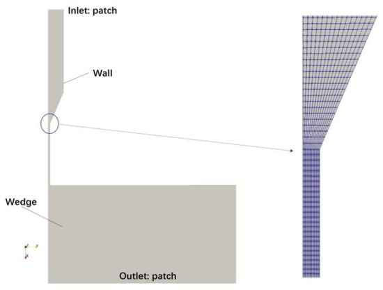
Figure 1.
Computational domain and local grid.
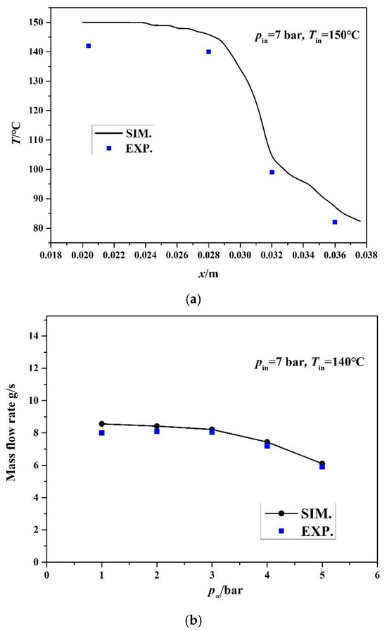
Figure 2.
Comparison between experiments and simulations. (a) Variation in pressure along the axis. (b) Mass flow rate of different ambient pressures.
In Figure 2a, a simulation was conducted to analyze the variation in pressure during the depressurization of the superheated water at the nozzle inlet at 150 °C. Although the simulated results are slightly higher than the experimental results, the overall trend is very similar. As shown in Figure 2b, the simulation captures the flow rate variation with ambient pressure at a 140 °C inlet temperature. The simulation successfully reproduces the observed phenomenon where the flow rate initially increases and reaches a steady state as the ambient pressure decreases. Despite this, there remains a disparity between the experimental and simulation results. There are several reasons for these discrepancies, including the simplicity of the domain and the empirical nature of the HRM parameters, which contribute to the inaccuracy of the simulation. Additionally, experimental measurements may have introduced uncertainties into the results.
4. Simulation Setup
Under the five topics discussed in this paper, there are primarily three sets of geometrical arrangements. The first set of structures represents a flashing tank equipped with a blast tube, where the pressure varies dramatically before and after the nozzle. There is a strong depressurization process involved, and shock waves occur within the blast tube to prevent damage to the tank bottom (Smith et al. [6]). Following the shock waves, the velocity decreases significantly. The second set portrays a flashing tank with a choke tube, where shock waves may occur within the tank. The exit diameter is then adjusted accordingly. The third set of structures involves studying the impact of the tube diameter and modifying the valve opening. The simulations utilize a 2D wedge geometry instead of a full 3D simulation to conserve computational resources. The wedge angle is set to 2 degrees (360° for three-dimensional simulations). Figure 3 depicts specific regions and structural dimensions. In Figure 3c, where ‘a’ represents the radius of the choke tube, and all other dimensions are normalized using ‘a’, the primary structures in Figure 3a through Figure 3c are similar. For instance, the tank’s height is 195.2a, the radius is 74a, the curvature at the bottom is 88a, and the exit diameter is 20a. In Figure 3b, the diameter of the choke tube is 1.52a, and under this condition, two different exit radii are simulated, namely, 1.2a and 2a. As shown in Figure 3c, the diameter of the choke tube is 2a, and a variety of valve opening configurations are simulated using the specific structures shown in the figure. There were certain simplifications made for the actual three-dimensional structures encountered in industrial applications in order to avoid the high complexity of the domain for this publication.
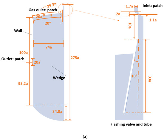
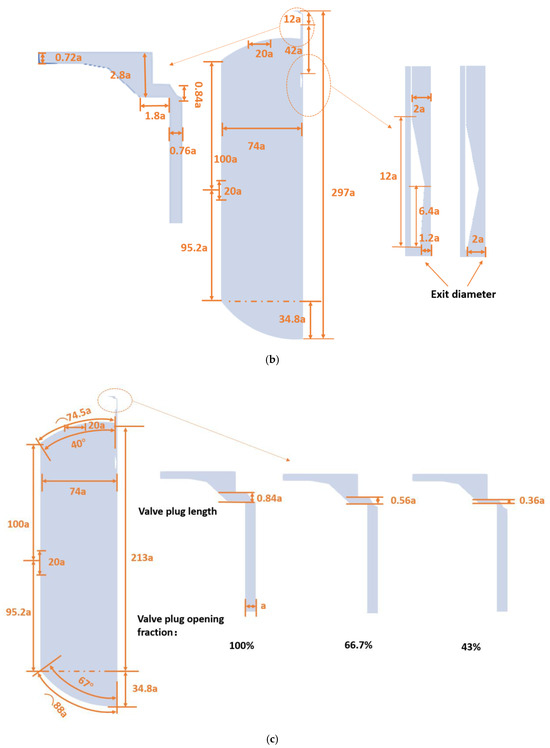
Figure 3.
Computational domain. (a) Blast tube structure. (b) Choke tube structure with a diameter of 1.52a. (c) Choke tube structure with a diameter of 2a.
The influence of grid refinement on velocity is illustrated in Figure 4 for the three different types of structures depicted in Figure 3. A total number of 25,375, 43,960, and 44,550 grid cells were found to be sufficient for producing accurate results.
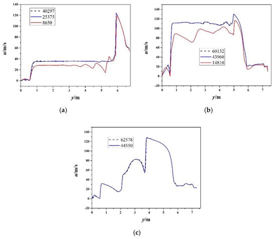
Figure 4.
Effect of the grid density on the velocity: (a) blast tube; (b) choke tube with a 1.52a diameter; (c) choke tube with a 2a diameter.
5. Application and Discussion
5.1. Blast Tube and Choke Tube
A first-stage flash vessel’s inlet slurry properties are provided in Table 1, while a last-stage flash vessel’s inlet slurry properties are provided in Table 2. Table 1 shows the initial conditions and slurry properties for Cases 1 and 2, and Table 2 shows those for Cases 3 and 4. The p0 represents the inlet pressure, p∞ denotes the initial ambient pressure, T0 signifies the inlet temperature, and αs0 represents the solid content. The material properties in the tables are sourced from the study by Smith et al. [6].

Table 1.
The properties of the inlet slurry of a first-stage flash vessel.
Table 2.
The properties of the inlet slurry of a last-stage flash vessel.
Figure 5a illustrates the velocity distribution within the blast tube under the operating conditions specified in Table 1. It has been observed that a shock wave inside the nozzle causes a significant reduction in velocity downstream of the wave. According to Figure 6a, a significant decrease in pressure inside the blast tube occurs at this point as the blast tube operates as a subsonic nozzle. Figure 5b illustrates the velocity distribution within the blast tube under the operating conditions specified in Table 2. As a result of the absence of shock waves within the blast tube, a long penetration mode jet is formed inside the vessel [29]. The results of this simulation indicate that there is a distinct instability and oscillation of the flow. There is no discernible region of velocity attenuation near the bottom of the vessel, which could potentially damage the flashing vessel. Additionally, in this scenario, the exit pressure of the nozzle is similar to the ambient pressure, only slightly higher, which results in the slurry maintaining a significant thrust at the exit while its velocity decays slowly within the tank. Therefore, if blast tubes are to be used under these conditions, it is imperative that the length of the expansion section within the blast tube be increased.
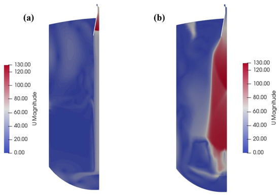
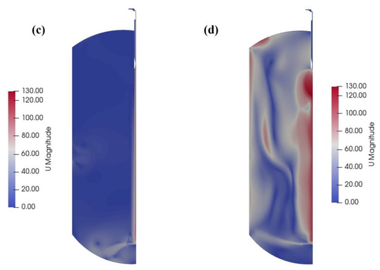
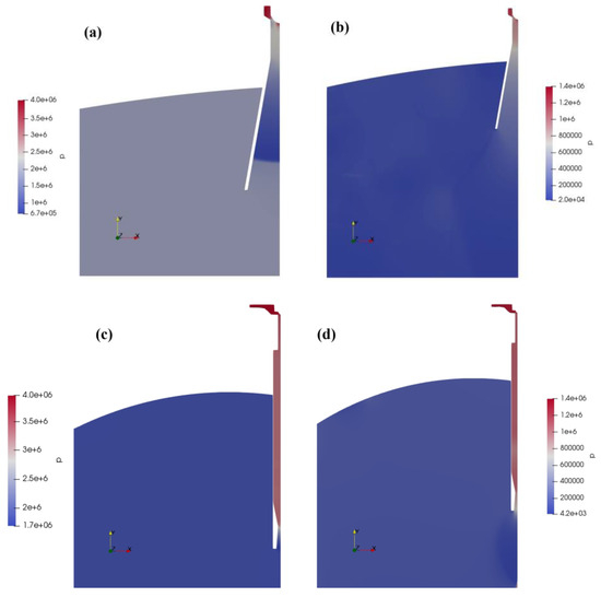
Figure 5c,d illustrates the simulation results for the slurry properties outlined in Table 1 and Table 2, respectively, using a choke tube configuration. It can be seen from Figure 5c that the jet velocity equals the axial velocity and remains consistent with the nozzle exit velocity. As depicted in Figure 6c, the static pressure at the exit is approximately equal to the ambient pressure of 18 bar. At this point, the jet is fully expanded, with the thrust at the outlet reaching its maximum and the exit velocity remaining unchanged as it impacts the bottom of the tank directly. However, the expansion range is relatively narrow, and the crash plate provides some protection for the vessel by covering the jet. However, the choke tube’s function becomes ineffective. According to Figure 5d, shock waves occur within the flashing vessel when using a choke tube, giving rise to shock diamonds [29], accompanied by highly unstable shear layers. In this case, the energy carried by the jet dissipates gradually. Therefore, despite being an under-expanded jet, the lateral range of the bottom velocity is narrow, and it falls within the crash plate, making the process relatively safe.
The blast tubes are designed to confine the shock waves within the tube. This significantly reduces the velocity at which the slurry enters the vessel. By using rigid ceramic materials, the blast tube prevents excessive velocities from damaging it. In the second design, shock waves are introduced into the tank via a choke tube, where energy is gradually dissipated by the interaction between the shock waves and surrounding air. This design requires control of the jet expansion to maintain the effectiveness of the crash plate. Both of these design approaches are closely related to the exit pressure and ambient pressure [30].
5.2. The Influence of Tube Diameter
In the case of choke tubes, the impact of the tube diameter on the slurry jetting behavior was investigated. As shown in Table 2, the initial conditions are described. Figure 7 shows the velocity field and Mach number distribution for tubes with diameters of 1.52a and 2a. The “shock diamonds” are formed inside the vessel when the tube diameter is 1.52a, and this pattern dissipates with increasing distance due to the friction at the contact discontinuity [29,31]. When the tube diameter is 2a, “barrel” shocks are formed within the vessel. This jet is characterized by the presence of a barrel-shaped expansion region at the nozzle, as shown schematically in Ref. [31], which culminates in a normal shock and Mach disc [32]. Moreover, the shape and magnitude of the shock waves can be adjusted by adjusting the nozzle exit pressure pexit and ambient pressure pambt. As proposed by Franquet et al. [33], shock waves with a pressure range of 1.1 ≤ pexit/pambt ≤ 3 are categorized as moderately under-expanded jets, indicating the presence of diamond-shaped shock waves. Conversely, shock waves with a pressure range of 2 ≤ pexit/pambt ≤ 4 appear as barrels, which are commonly referred to as highly under-expanded jets. These shock waves are generated by the pressure of the slurry at the tube exit being significantly higher than the surrounding ambient pressure, which is a characteristic of an under-expanded jet. In this case, the flow continues to expand outward once it exits the tube, leading to an increase in its velocity and Mach number within the tank. Consequently, there is no conversion of energy into thrust in this process.
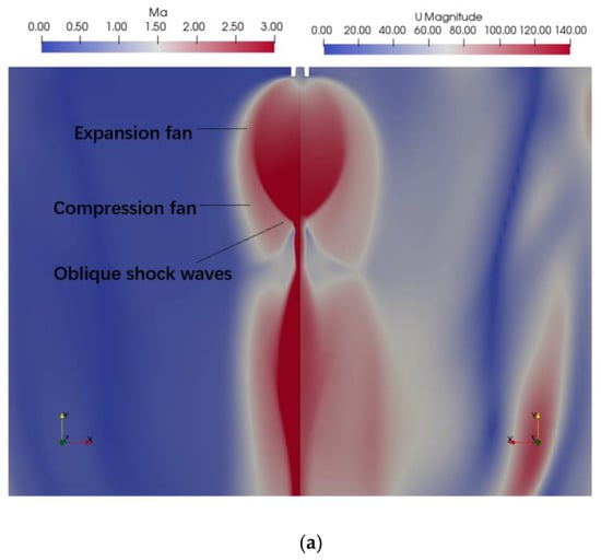
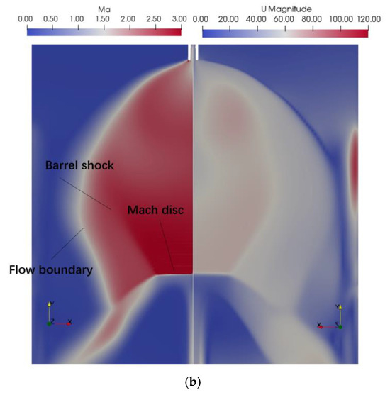
Figure 7.
Distribution of velocity (m/s) and Mach number in choke tubes with different diameters. (a) 1.52a and (b) 2a.
According to the authors, controlling the vessel height manages the longitudinal extension ranges of diamond-shaped shocks and gradually diminishes wave intensity. The safety requirements can be satisfied by increasing the vessel height and implementing a properly designed crash plate at the bottom. In the case of barrel shocks, an excessive shock wave width can pose a safety hazard by impacting the sidewalls; therefore, an increase in vessel width is necessary. To ensure the safe operation of a choke tube with a larger diameter, advanced planning is required. For instance, controlling the valve opening can enhance safety.
5.3. The Influence of Valve Opening
According to Section 5.2, a larger tube diameter facilitates more efficient handling of slurry. It is therefore possible to modulate the valve opening to control barrel shock. Based on the initial conditions presented in Table 2, three distinct valve opening configurations were selected, including 100%, 66%, and 43%. For each setting of the valve opening, Figure 8 illustrates the gradual formation of the shock wave. Based on Figure 8a, the limited space within the vessel, which corresponds to the fully open valve condition, causes the expansion fan to collide with the side wall, resulting in elevated velocity at the bottom of the vessel. As shown in Figure 8b, the shock wave progresses into a complete barrel shape when the valve opening is set at 66%. It can be seen from Figure 8c that there is a small discrepancy between the valve opening of 43% and the valve opening of 66%. In Figure 8a–c, there is also a trend indicating that the expansion fan range initially decreases and eventually reaches a stable state as the valve opening decreases.
Figure 8.
Distribution of velocity (m/s) in choke tubes with different valve openings. (a) 100%. (b) 66%. (c) 43%.
In order to provide a more detailed understanding of how the slurry’s velocity distribution affects the tank walls during operation, a more detailed analysis was conducted for the three shock wave states shown in Figure 8. As shown in Figure 9, a velocity streamline chart was used to systematically assess the maximum impact on the side walls and bottom of the vessel. When the valve was opened to 100%, the maximum ux impacting the side walls was 37.07 m/s, whereas the maximum uy reaching the bottom was 70.88 m/s. The maximum ux hitting the side walls decreased to 22.42 m/s when the valve opening was reduced to 66%, whereas the maximum uy hitting the bottom decreased to 33.93 m/s. The maximum ux impacting the side walls at a valve opening of 43% was 23.53 m/s, while the maximum uy impacting the bottom was 33.95 m/s. These findings suggest that a tube diameter of 2a, coupled with a valve opening of 66%, exhibits relatively stable performance. Based on mass conservation and the calculation for mass flow rate (), the achievable mass flow rate for the configuration with a tube diameter of 2a is 25.5 kg/s, while the configuration with a tube diameter of 1.52a enables 16.7 kg/s. Additionally, varying the valve opening from 100% to 43% resulted in only a slight reduction in the jet range.
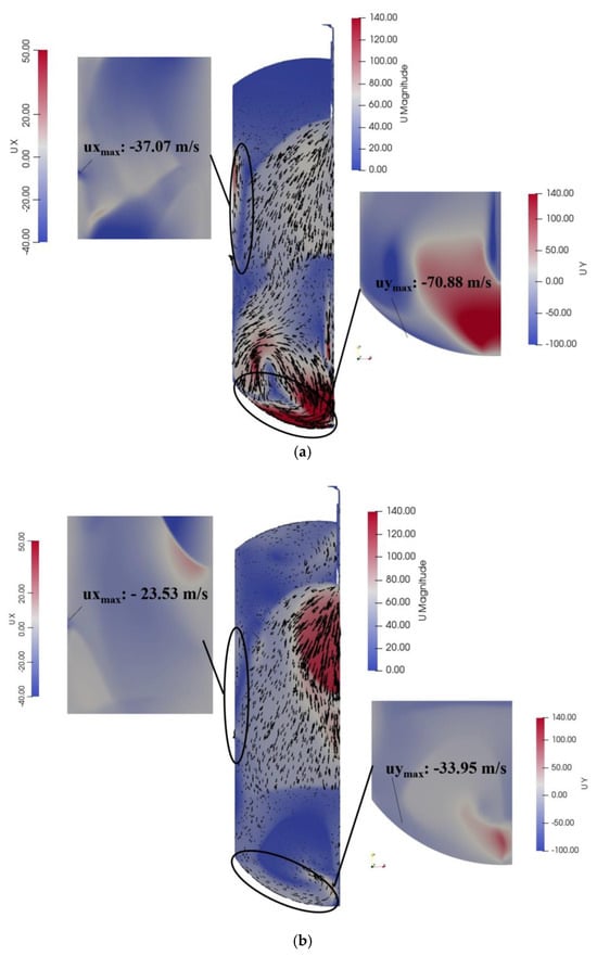
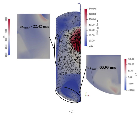
Figure 9.
Velocity streamline chart in choke tubes with different valve openings. (a) 100%. (b) 66%. (c) 43%.
5.4. The Influence of Exit Diameter
The present study investigated the effect of the exit diameter on the spray range. Under the initial conditions as outlined in Table 2, the tube diameter was fixed at 1.52a, while the exit diameter was examined at 2.4a and 4a. As shown in Figure 10, the corresponding results for the half-radial spread of spray (SW) and velocity are presented.
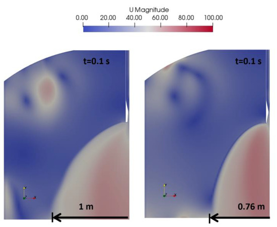
Figure 10.
Distribution of velocity (m/s) in choke tubes with different exit diameters.
With an increase in the exit diameter, the SW decreased from 1 m to 0.76 m, indicating a reduction in the lateral dispersion of the spray. A slight increase in the outlet velocity was also observed with an increasing exit diameter. It is therefore recommended to consider an appropriate enlargement of the exit diameter to minimize lateral wall collisions.
5.5. The Influence of Backpressure
According to the jet discharge mechanism and shock wave generation principle [28], it is evident that varying backpressure will result in changes in the position and expansion of shock waves, thereby affecting the spray angle, outlet velocity, and processing flow rate. In the initial conditions presented in Table 2 of this study, the pressure variations are substantial, resulting in the formation of consecutive shock waves within the tank. An improper operation under such circumstances may result in a safety accident. Thus, the purpose of this section is to investigate the flow patterns inside the tank under various backpressure conditions.
According to Figure 11, as the backpressure increases, the SW decreases significantly, so that at a backpressure of 6 bar, no shock waves are generated within the tank. This characteristic can be attributed to the decrease in the ratio between the exit pressure and the ambient pressure with increasing backpressure. Consequently, the jet flow transitions from an under-expanded jet to a fully expanded jet, as indicated in the partial pressure distribution in Figure 11. Due to this, it is common to use multiple flashing tanks connected in series for stepwise pressure release in flashing units. Furthermore, as the backpressure increases to 6 bar, the jet becomes a fully expanded jet, rendering the choke tube ineffective. Consequently, an excessively high backpressure should be avoided in the design as it can result in equipment consumption.
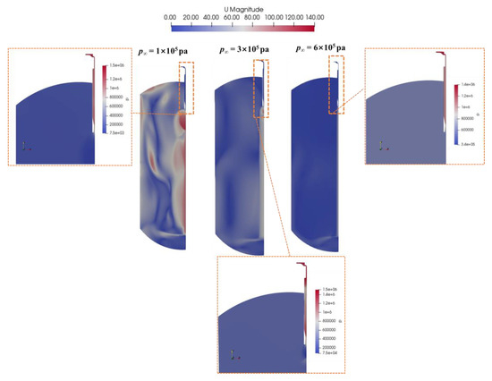
Figure 11.
Distribution of velocity (m/s) and partial pressure (Pa) in choke tubes with different backpressures.
6. Conclusions
In this study, CFD has been used to study the influence of flashing tank design and operating parameters on fluid behavior within a flashing unit. Analysis of the velocity and pressure fields under different working conditions will provide insights into optimal and safe operational practices. The simulation results demonstrate that blast tubes are designed to control the shock waves in the expansion section and reduce velocity at the nozzle exit. On the other hand, choke tubes are designed to dissipate shock waves gradually and steadily. When using larger choke tube diameters, flow rates increase, but this also shifts the shock patterns from a diamond to a barrel shape, necessitating wider tanks for safety. A barrel shock wave’s expansion fan range relates to the valve opening in the choke tube. By reducing the opening, the expansion fan gradually decreases until it stabilizes. Increasing the backpressure values can control the extent of the expansion of the jet and thus affect the shock wave position and expansion range. This may enhance the stability of the device to some extent. Nevertheless, excessively high backpressure can result in an increase in economic costs due to the addition of more flashing tanks.
Author Contributions
Conceptualization, B.K.; Methodology, Y.X.; Investigation, H.X.; Data curation, Z.P.; Writing—original draft, Y.X.; Data curation, C.X.; Data curation, X.W.; Data curation, Q.L. All authors have read and agreed to the published version of the manuscript.
Funding
This research was funded by Shantou Science and Technology Bureau grant number 211210147160630 and the APC was funded by Guangdong Department of Education Key Discipline Fund 2023.
Data Availability Statement
Due to privacy and ethical constraints, we regret that we are unable to provide access to the raw research data supporting the reported results in this study. We appreciate your understanding of these limitations and are available to address any specific questions or concerns related to our research.
Conflicts of Interest
The authors declare no conflict of interest.
References
- Gu, G.; Gao, T. Sustainable Production of Lithium Salts Extraction from Ores in China: Cleaner Production Assessment. Resour. Policy 2021, 74, 102261. [Google Scholar] [CrossRef]
- Meng, F.; McNeice, J.; Zadeh, S.S.; Ghahreman, A. Review of Lithium Production and Recovery from Minerals, Brines, and Lithium-Ion Batteries. Miner. Process. Extr. Metall. Rev. 2021, 42, 123–141. [Google Scholar] [CrossRef]
- Chagnes, A.; Pospiech, B. A Brief Review on Hydrometallurgical Technologies for Recycling Spent Lithium-Ion Batteries. J. Chem. Technol. Biotechnol. 2013, 88, 1191–1199. [Google Scholar] [CrossRef]
- Salakjani, N.K.; Singh, P.; Nikoloski, A.N. Production of Lithium—A Literature Review. Part 2. Extraction from Spodumene. Miner. Process. Extr. Metall. Rev. 2021, 42, 268–283. [Google Scholar] [CrossRef]
- Liu, J.; Liu, B.; Zhou, P.; Wu, D.; Wu, C. An Overview of Flashing Phenomena in Pressure Hydrometallurgy. Processes 2023, 11, 2322. [Google Scholar] [CrossRef]
- Smith, C.C.; Dixon, D.G.; Luque, M.R.; Robison, J.C.; Chipman, S.R. Analysis and Design of Flashtubes for Pressure Letdown in Autoclave Leaching Operations. Hydrometallurgy 2006, 81, 86–99. [Google Scholar] [CrossRef]
- Liao, Y.; Lucas, D. 3D CFD Simulation of Flashing Flows in a Converging-Diverging Nozzle. Nucl. Eng. Des. 2015, 292, 149–163. [Google Scholar] [CrossRef]
- Blackmore, A.; Shah, U.; Pearson, M.; Plikas, A.; Sim, B. Flashing of Pressurized Slurry in Metallurgical Processing: A Review of the State of the Art, Operational Experiences, and Recommendations for Future Research. In Proceedings of the Fluids Engineering Division Summer Meeting, Chicago, IL, USA, 3–7 August 2014; p. V01DT32A013. [Google Scholar] [CrossRef]
- Fluerenbrock, F. Pressure Gradient and Choking Velocity for Adiabatic Pipe Flow of a Homogeneous Steam-Water-Solids Mixture. J. Fluids Eng. Trans. ASME 2000, 122, 769–773. [Google Scholar] [CrossRef]
- Fuster, D.; Hauke, G.; Dopazo, C. Influence of the Accommodation Coefficient on Nonlinear Bubble Oscillations. J. Acoust. Soc. Am. 2010, 128, 5–10. [Google Scholar] [CrossRef]
- Zwart, P.; Gerber, A.G.; Belamri, T. A Two-Phase Flow Model for Predicting Cavitation Dynamics. In Proceedings of the Fifth International Conference on Multiphase Flow, Yokohama, Japan, 30 May–4 June 2004. [Google Scholar]
- Bilicki, Z.; Kestin, J. Physical Aspects of the Relaxation Model in Two-Phase Flow. Proc. R. Soc. London. A Math. Phys. Sci. 1990, 428, 379–397. [Google Scholar]
- Karathanassis, I.K.; Koukouvinis, P.; Gavaises, M. Comparative Evaluation of Phase-Change Mechanisms for the Prediction of Flashing Flows. Int. J. Multiph. Flow 2017, 95, 257–270. [Google Scholar] [CrossRef]
- Downar-Zapolski, P.; Bilicki, Z.; Bolle, L.; Franco, J. The Non-Equilibrium Relaxation Model for One-Dimensional Flashing Liquid Flow. Int. J. Multiph. Flow 1996, 22, 473–483. [Google Scholar] [CrossRef]
- Neroorkar, K.; Shields, B.; Grover, R.O.; Plazas Torres, A.; Schmidt, D. Application of the Homogeneous Relaxation Model to Simulating Cavitating Flow of a Diesel Fuel; SAE Technical Paper; SAE International: Warrendale, PA, USA, 2012. [Google Scholar] [CrossRef]
- Gärtner, J.W.; Kronenburg, A.; Rees, A.; Sender, J.; Oschwald, M.; Lamanna, G. Numerical and Experimental Analysis of Flashing Cryogenic Nitrogen. Int. J. Multiph. Flow 2020, 130, 103360. [Google Scholar] [CrossRef]
- Lee, J.; Madabhushi, R.; Fotache, C.; Gopalakrishnan, S.; Schmidt, D. Flashing Flow of Superheated Jet Fuel. Proc. Combust. Inst. 2009, 32, 3215–3222. [Google Scholar] [CrossRef]
- Neroorkar, K.D. Modeling of Flash Boiling Flows in Injectors with Gasoline-Ethanol Fuel Blends. Ph.D. Thesis, University of Massachusetts Amherst, Amherst, MA, USA, 2011. [Google Scholar]
- Mohan, B.; Badra, J.; Sim, J.; Im, H.G. Coupled In-Nozzle Flow and Spray Simulation of Engine Combustion Network Spray-G Injector. Int. J. Engine Res. 2021, 22, 2982–2996. [Google Scholar] [CrossRef]
- Saha, K.; Som, S.; Battistoni, M. Investigation of Homogeneous Relaxation Model Parameters and Their Implications for Gasoline Injectors. At. Sprays 2017, 27, 345–365. [Google Scholar] [CrossRef]
- Linstorm, P. Nist Chemistry Webbook, Nist Standard Reference Database Number 69. J. Phys. Chem. Ref. Data Monogr. 1998, 9, 1–1951. [Google Scholar]
- Herrig, S. New Helmholtz-Energy Equations of State for Pure Fluids and CCS-Relevant Mixtures. Ph.D. Thesis, Ruhr-Universität Bochum, Bochum, Germany, 2018. [Google Scholar]
- Xiao, Y.; Cheng, T.; Pan, Z.; Kong, B. CFD Simulations for Flashing Pressurized Slurry in Metallurgical Processing. Hydrometallurgy 2023, 222, 106154. [Google Scholar] [CrossRef]
- Andreopoulos, Y.; Agui, J.H.; Briassulis, G. Shock Wave–Turbulence Interactions. Annu. Rev. Fluid Mech. 2020, 32, 309–345. [Google Scholar]
- Ali Pasha, A.; Sinha, K. Shock-Unsteadiness Model Applied to Oblique Shock Wave/Turbulent Boundary-Layer Interaction. Int. J. Comut. Fluid Dyn. 2008, 22, 569–582. [Google Scholar] [CrossRef]
- Schmidt, D.P.; Gopalakrishnan, S.; Jasak, H. Multi-Dimensional Simulation of Thermal Non-Equilibrium Channel Flow. Int. J. Multiph. Flow 2010, 36, 284–292. [Google Scholar] [CrossRef]
- Weller, H.G.; Tabor, G.; Jasak, H.; Fureby, C. A Tensorial Approach to Computational Continuum Mechanics Using Object-Oriented Techniques. Comput. Phys. 1998, 12, 620–631. [Google Scholar] [CrossRef]
- Wirth, K.E.; Rossmeissl, M. Critical Mass-Flow in Orifice-Nozzles at the Disintegration of Superheated Liquids. In Proceedings of the ASME 2006 2nd Joint U.S.-European Fluids Engineering Summer Meeting Collocated with the 14th International Conference on Nuclear Engineering. Volume 1: Symposia, Parts A and B, Miami, FL, USA, 17–20 July 2006; Volume 98043, pp. 1381–1388. [Google Scholar] [CrossRef]
- Daso, E.O.; Pritchett, V.E.; Wang, T.S.; Ota, D.K.; Blankson, I.M.; Auslender, A.H. Dynamics of Shock Dispersion and Interactions in Supersonic Freestreams with Counterflowing Jets. AIAA J. 2009, 47, 1313–1326. [Google Scholar] [CrossRef]
- Yin, P.; Yang, S.; Li, X.; Xu, M. Numerical Simulation of In-Nozzle Flow Characteristics under Flash Boiling Conditions. Int. J. Multiph. Flow 2020, 127, 103275. [Google Scholar] [CrossRef]
- White, T.R.; Milton, B.E. Shock Wave Calibration of Under-Expanded Natural Gas Fuel Jets. Shock Waves 2008, 18, 353–364. [Google Scholar] [CrossRef]
- Ewan, B.C.R.; Moodie, K. Structure and Velocity Measurements in Underexpanded Jets. Combust. Sci. Technol. 1986, 45, 275–288. [Google Scholar] [CrossRef]
- Franquet, E.; Perrier, V.; Gibout, S.; Bruel, P. Free Underexpanded Jets in a Quiescent Medium: A Review. Prog. Aerosp. Sci. 2015, 77, 25–53. [Google Scholar] [CrossRef]
Disclaimer/Publisher’s Note: The statements, opinions and data contained in all publications are solely those of the individual author(s) and contributor(s) and not of MDPI and/or the editor(s). MDPI and/or the editor(s) disclaim responsibility for any injury to people or property resulting from any ideas, methods, instructions or products referred to in the content. |
© 2023 by the authors. Licensee MDPI, Basel, Switzerland. This article is an open access article distributed under the terms and conditions of the Creative Commons Attribution (CC BY) license (https://creativecommons.org/licenses/by/4.0/).