Article

Study on Connectivity Analysis and Injection–Production Optimization of Strong Heterogeneous Sandstone Reservoir Based on Connectivity Method

1
School of Petroleum Engineering, Yangtze University, Wuhan 430100, China
2
Western Research Institute, Yangtze University, Karamay 834000, China
3
Key Laboratory of Drilling and Production Engineering for Oil and Gas, Wuhan 430100, China
4
Luliang Oilfield Operation Area, Xinjiang Oilfield Company, PetroChina, Karamay 834000, China
5
The 10th Oil Production Plant, Changqing Oilfield Company, PetroChina, Qingcheng 745100, China
6
Army Logistics Academy, Chongqing 401311, China
*
Author to whom correspondence should be addressed.
Processes 2023, 11(10), 2816; https://doi.org/10.3390/pr11102816
Submission received: 27 August 2023 / Revised: 13 September 2023 / Accepted: 21 September 2023 / Published: 22 September 2023
(This article belongs to the Special Issue Advances in Enhancing Unconventional Oil/Gas Recovery)

Abstract

:
The D reservoir in the Bongor Basin, southern Chad, is highly heterogeneous. In the stage of waterflood development, the injected water is seriously channeled along the dominant channel, and the water drive effect becomes worse. At the same time, due to the strong edge and bottom water, the water flooding situation is aggravated, the water cut is increased, and the development efficiency is reduced. To accurately identify the inter-well connectivity relationship, we developed a reservoir inter-well connectivity model based on the principle of inter-well connectivity and dynamic production data and reservoir geological parameters. Thus, the plane water injection split coefficient and water injection efficiency of each reservoir layer were obtained. The results are in good agreement with the calculation results of inter-well connectivity through verification with field tracer interpretation. The practical application results show that the method can increase the annual output of oil by 1.3%, which has a good oil increase effect. In this study, a model of inter-well connectivity in multi-layer sandstone reservoirs was established for the first time. The production performance of the model injection–production well was optimized in real time by a historical fitting and production optimization algorithm and then applied to real reservoirs, so that it could effectively improve the oilfield development and optimize the injection–production structure.

1. Introduction

Water injection development is the main development method of major oil fields at present. After a long period of water injection, major oil fields have gradually entered the middle and high water cut periods [1]. After years of waterflooding development, the oil production rate of the D block in Chad, Africa has been continuously reduced. At the same time, due to the strong heterogeneity of the reservoir, water channeling is serious in the process of water flooding development. Moreover, due to the influence of strong edge and bottom water, water flooding occurs in multiple wells, the water content rises, and the development efficiency is reduced. Thus, how to combine the existing understanding of reservoirs, quickly formulate a targeted and effective block injection–production optimization plan, adjust the injection–production structure, and improve the current situation of reservoir development is the main problem that needs to be solved urgently. Accurately identifying the injection–production connectivity between production wells and injection wells is an important factor affecting the injection–production effect. As an important research method, the inter-well connectivity method can effectively identify the connectivity between oil and water wells.
In recent years, research on inter-well connectivity has mainly been carried out from both static and dynamic aspects. The study of static connectivity is usually to evaluate the initial state before reservoir development. At present, numerous methods have been developed to describe and evaluate the static connectivity of reservoirs, including the micro-seismic analysis method, logging interpretation method, geological modeling method, and reservoir parameter analysis method. The micro-seismic analytical method mainly analyzes the structure and properties of underground rock strata by using the velocity difference of seismic waves propagating in different rock strata. Liu et al. [2] proposed a method for evaluating fracture-well connectivity in fractured sandstone reservoirs by using micro-seismic monitoring technology and tracer analysis results, and quantitatively evaluated fracture-well connectivity. Mammad Mirzayev et al. [3] analyzed the key factors affecting the development of water flooding based on the connectivity index, and combined the results of geological and seismic analysis for correlation analysis. The logging interpretation method is one of the important means to evaluate the static inter-well connectivity of reservoirs. It mainly obtains information on rock physical parameters, permeability, and porosity, and then establishes the relevant logging model to judge the connectivity between oil and water wells. Qu et al. [4] analyzed the change in reservoir plane heterogeneity by the logging interpretation static method, and found that the reservoir plane heterogeneity in the well area of the Bohai L oilfield is strong. Zhang et al. [5] studied the pore and fracture development characteristics of the deep Sinian Dengying Formation reservoir in the Sichuan Basin by logging methods, and the application of logging methods in evaluating reservoir effectiveness. The reservoir parameter analysis method infers the fluid connectivity between different wells by analyzing the differences in oil and gas composition and physical parameters of different wells. Patidar et al. [6] analyzed the relative content of alkanes such as C1–C5 by gas chromatography and liquid chromatography. Zhang et al. [7] evaluated the reservoir properties and inter-well static connectivity of different well sections by analyzing the parameters such as liquid production, gas production, and water content of different well sections. The geological modeling method divides the reservoir into different phases by analyzing factors such as reservoir rock type, pore structure, and pore connectivity. Fang et al. [8] proposed a phase model to describe the physical properties of sedimentary rocks. Through a phase analysis, the connectivity of pores in the reservoir can be judged more accurately. Ye et al. [9] proposed a well seismic four-in-one reservoir-modeling method to improve the accuracy of the geological model in the later stage of oilfield development.
Although the static method is mostly simple when evaluating inter-well connectivity, it cannot accurately characterize the changes in the process of reservoir oil and gas migration. Through the study of dynamic connectivity, we can more accurately understand the flow path and speed of oil and gas in the reservoir at different times and different locations. When the reservoir changes, we can also grasp its evolution law over time. At present, numerous methods have been established to describe and evaluate the dynamic connectivity between wells. These include the tracer analysis method, numerical simulation method, and dynamic data inversion method. Tracer analysis is a method to study the transmission and mixing process of fluid in underground reservoirs. It is one of the most commonly used methods for evaluating inter-well dynamic connectivity. Cao et al. [10] quantitatively evaluated the dynamic connectivity between injection and production wells by analyzing the parameters of tracer time, concentration, continuous seeing time, and peak concentration in the benefit wells. Chen et al. [11] studied the inter-well connectivity of the injection–production well group in the Suizhong 36-1 oilfield by using the inter-well trace substance tracer technology, which provided quantitative technical parameters for the effective development of the oilfield in the later stage. Yu et al. [12] used the multi-component definition function of CMG 2017 numerical simulation software to match the history of single-well polymer production mass concentration, and realized the identification of the polymer production direction and the analysis of the output. Li et al. [13] quantitatively characterized the high-permeability channel and reservoir heterogeneity in the Changqing Oilfield by comprehensively analyzing the results of trace substance tracer monitoring and reservoir numerical simulation. Albertoni et al. [14] used the multiple linear regression model combined with the diffusion filter to clarify the main factors affecting the inter-well connectivity and quantitatively characterize the inter-well connectivity. Yousef et al. [15] proposed a capacitance–resistance model based on material balance, and Sayarpour et al. [16] proposed three improved capacitance–resistance models based on the research of the capacitance–resistance model. Based on the multi-well productivity index method, Kaviani et al. [17] evaluated the inter-well dynamic connectivity by considering the dynamic production factors such as location, skin factor, injection rate, and bottom hole flowing pressure. Based on the dynamic production data of injection–production wells, Liu et al. [18] used the combination of the Kalman filter and an artificial neural network to quantitatively characterize the dynamic connectivity between reservoirs. However, the calculation speed and accuracy of these models are slow, and they cannot consider many complex cases at the same time. Thus, Zhao et al. [19,20] proposed a connectivity model that does not depend on complex fine modeling. The reservoir injection–production system is simplified by the inter-well conductivity and connected volume. Modeling and simulation calculations are carried out by using dynamic reservoir production data and geological parameters. On this basis, the reservoir production optimization control model is established. By optimizing the injection–production structure, the injection–production optimization scheme design is completed to guide the field production application.

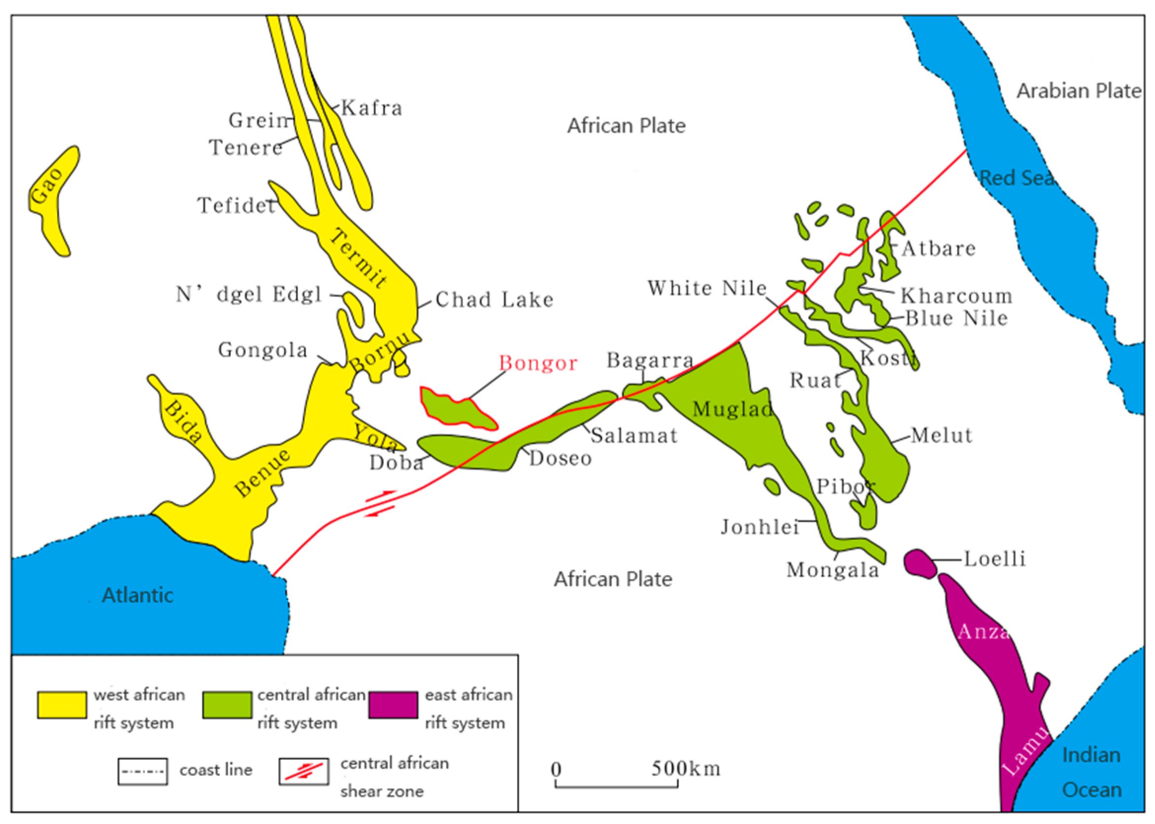
2. Geological Setting and Field Example

The Bongor Basin is located at the intersection of the Central African and West African rift systems, southwest of the Republic of Chad, and the northern margin of the Central African shear zone [21,22,23] (Figure 1). It is a meso-Cenozoic intracontinental inversion rift basin developed under the influence of the Central African shear zone. The sedimentary characteristics of the Bongor Basin reservoir mainly include five categories: gray siltstone, gray claystone, gray mudstone, gray-brown sandstone, and gray-green sandstone. These reservoirs have good porosity and permeability and are important oil and gas reserves in the Bongor Basin. The D block reservoir is located in the Bongor basin, which is an edge–bottom water reservoir controlled by structural lithology. The buried depth in the middle of the reservoir is 1270 m, and the reservoir is thick in the middle and thin at both ends. From top to bottom, the reservoir is more developed.

3. Reservoir Inter-Well Connectivity Model

The conductivity and connected volume in the inter-well connectivity model proposed by Zhao Hui represent the flow capacity and material basis of the reservoir unit, respectively. The simulation calculation takes less time and the history matching accuracy is higher. However, at present, the application scenarios of this method are mostly single-layer sandstone reservoirs and have not been effectively extended to multi-layer sandstone reservoirs.
Therefore, based on the theory of inter-well connectivity [24], this paper will apply the method to multi-layer sandstone reservoirs. Through the characteristic production and development parameters of D reservoir in Chad, a multi-layer inter-well connectivity model is constructed to finely characterize the injection–production relationship between multi-layer injection wells and production wells in the study area. Using field tracer data to analyze and adjust the inter-well conductivity and connectivity volume values, the inter-well connectivity field is obtained in real-time. Finally, according to the average water injection efficiency of the water injection wells in the study block, each water injection well is divided into high-efficiency wells and low-efficiency wells. Through the optimization algorithm, the optimal control of the injection volume of the water injection well is realized, and the purpose of controlling water-increasing oil and identifying the dominant channel of the reservoir is achieved.

3.1. Model Moisture Content Solution

Considering the oil–water two-phase flow under adiabatic conditions, ignoring the influence of gravity, the viscosity of the fluid remains constant. Based on this, the material balance equation is established:
j = 1 n c , i T i , j ( p j ( t ) p i ( t ) ) + q i ( t ) = d p i ( t ) d t c t , i ( t ) V p , i ( t )
In Formula (1), n c , i represents the number of wells connected to well i ; the unit q i ( t ) is m3/d. It represents the inflow and outflow liquid volume of the source and sink phase of the i th well under reservoir conditions. If well i is a production well, then the liquid volume is positive. If it is a water injection well, then the liquid volume is negative. p i is the average pressure of the connected unit V P , i . c t , i is the comprehensive compression coefficient of well i . The IMPES (implicit pressure explicit saturation) scheme is used to rewrite the formula, and the difference scheme is obtained as follows:
p i n p i n 1 = Δ t n c t , i n 1 V p , i n 1 ( ( j = 1 n c , i T i , j n 1 ) p i n + j = 1 n c , i T i , j n 1 p j n + q i n 1 )
among them,
T i , j n 1 = 11.57 A i , j λ i , j n 1 L i , j = T i , j 0 λ i , j n 1 λ i , j 0
V p , i n 1 = V p , i 0 ( 1 + C t , i ( p i n 1 p i 0 ) )
C t , i n 1 = C r + S w , i n 1 C w + S o , i n 1 C o
In Formulas (3)–(5), A i , j and L i , j are the seepage cross-sectional area between well i and well j and the length of the connected unit, respectively, and the units are m2 and m. T i , j 0 and T i , j n 1 refer to the conductivity value between well i and well j at the initial time and time n − 1; m3·d−1·MPa−1. V p , i 0 and V p , i n 1 refer to the control volume of well i at the initial time and the n − 1 time point; m3. λ i , j 0 and λ i , j n refer to the mobility value between well i and well j at the initial time and time n − 1, respectively; 10−3 μm2·(mPa·s)−1. C t , C w , and C o refer to the compression coefficient of reservoir rock, reservoir crude oil, and reservoir water; MPa−1. S w , i and S o , i refer to the water saturation and oil saturation at well i . The formula in [25] can be obtained by the implicit difference discrete calculation of the Formula (1). The average pressure value of the single-well control area of each well at any time is obtained, and the flow rate in the connected unit is obtained by combining the conductivity between wells.
q i , j n = T i , j n ( p j n p i n )
In Formula (6): q i , j n is the flow rate from well j to well i ; m3/s.
Considering the influence of edge and bottom water in the reservoir, it is deduced according to the theory of front edge propulsion [26,27,28]. By setting an upstream node position x u of x , the saturation of the corresponding node position is S w u , and it is concluded that:
f w S w = f w S w u + 1 Q D n
In Formula (7): f w S w is the derivative of water content at x u ; Q D n represents the dimensionless cumulative injection amount from x u to x at time n; f w S w represents the water content derivative of the reservoir unit at position x .
According to the above calculation results, the water cut derivative corresponding to well j tracking to downstream well i at time n can be obtained:
f w S w n i j = min f w S w n j + 1 Q D n i j , f w S w k i Q D k i j Q D n j i
In Formula (8), f w S w n j and f w S w k i represent the derivative of water content at well j and i at time n and k , respectively; Q D n i j and Q D n j i denote the dimensionless cumulative flow from well j to well i and the dimensionless cumulative flow from well i to well j at time n, respectively. Q D k i j is the dimensionless cumulative flow from well i to well j at time k .
The interpolation calculation of Formula (8) is carried out to obtain the water content of well i from the direction of well j , and then the respective water content in the upstream direction is obtained. Finally, the water content of well i at time n can be obtained:
f w S w n i = j = 1 m q i j f w S w n i j j = 1 m q i j
In Formula (9): f w S w n i represents the comprehensive water cut of well i .

3.2. Connectivity Parameter Inversion

By continuously updating, adjusting, and optimizing the connected parameter values, namely the connected volume and the connected conductivity, the calculated block cumulative oil production, block water content, single-well oil production, single-well water content, and other production dynamics are historically matched. The connected characteristic parameter matrix c is solved by using the random disturbance and projection gradient algorithm [29] so that the objective function O c can obtain the minimum value.
O c = 1 2 c c r T K B 1 c c r + 1 2 m o b s h c T K D 1 m o b s h c ( c 0 )
In Formula (10): c denotes the connected parameter matrix; c r represents the prior feature parameter model estimation; K B 1 represents the inverse covariance matrix of the model parameters; m o b s denotes the measured data; K D 1 is the covariance matrix of the prior model characteristic parameters; h b is the initial value of the results calculated by the reservoir numerical simulator. At the same time, the constraint conditions are iteratively solved:
c l + 1 = c l η Τ l c l
In Formula (11): c l + 1 is the iteration variable of step l + 1; η represents the search step size; T represents the N u -dimensional projection matrix; l c l is the random perturbation gradient of O c .
The stochastic disturbance gradient of the objective function can be calculated by the following formula:
l c l = O c l + ε l Δ l O c l ε l × Δ l
In Formula (12): ε l denotes the gradient perturbation step; Δ l denotes a N u -dimensional random perturbation vector.

3.3. Calculation of Water Injection Splitting Efficiency

After the inversion of the connectivity parameters, the dynamic parameters of the oil and water wells can be obtained by calculation [30], and the dynamic parameters change with the change of the actual working system. According to the connected model after history matching, the stratified cumulative splitting coefficient and instantaneous splitting coefficient of the water well at the corresponding time, the stratified oil production and liquid production of the oil well [31], and other data are calculated.
Assuming that well i is an injection, the water distribution coefficient of the surrounding production well j is calculated to be α n i j , which is expressed as:
α n i j = q i j j = 1 m q i j
According to the above calculation results, the average water injection and oil displacement efficiency of the block at the last moment of reservoir development is calculated:
φ w = i = 1 m q i 1 f w i j = 1 m q j
In Formula (14): φ w represents the average water injection splitting efficiency; f w i represents the water content of well i .
The oil displacement efficiency of the water injection well indicates the amount of crude oil displaced from the oil well by the unit of water injected into the water injection well. In the case of the same amount of water being injected into the water injection well, less crude oil is displaced, indicating that the oil displacement efficiency of the water injection well to the oil well is lower, indicating that there may be channeling channels around the corresponding well, and ineffective water flooding is serious; on the contrary, if the oil displacement efficiency is higher, then the amount of crude oil displaced is more, and the production situation is better. Therefore, the stratified water injection efficiency is introduced to represent the water injection efficiency of the water injection well in each layer:
φ w i k = t = 0 n j = 1 m q i , n B i j k , n ( 1 f w j k , n ) t 0 n q i , n B i k , n
In Formula (15): φ w i k represents the water injection efficiency of well i in the kth layer; B i j k , n denotes the splitting component of liquid production of well i in k layers at time n; B i k , n denotes the splitting coefficient of water injection from well i to well j in layer k at time n.
The average water injection efficiency of the water injection well is compared with the water injection efficiency of each layer of the single well. If the water injection efficiency of the single well is less than the average water injection efficiency of the block, then the water injection well is reduced; otherwise, the water injection is increased. At the same time, based on the updated water injection well scheme, the water injection system of the water injection well to each production well is adjusted, and the injection–production structure is adjusted to reduce the water flooding and water channeling. The specific design process is as follows.
(1) The average water injection efficiency of the block at the last moment of reservoir development is calculated and used as a criterion for judging high-efficiency wells and low-efficiency wells. The specific calculation formula is Formula (14).
(2) Efficiency evaluation and analysis of water injection wells: If the injection well φ w i k > φ w , then it is judged that the water injection efficiency is high and the injection needs to be increased. On the contrary, if φ w i k < φ w , then the water injection efficiency is low, and the water injection needs to be reduced. After optimization, the water injection volume of each layer of the water injection well is as follows:
q i k n e w = q i k 1 + W i k ;
among them.
W i k = W min φ φ w i k φ φ min γ , φ w i k φ W max φ w i k φ φ max φ γ , φ w i k < φ
The upper limit W min is set to 0.4, the lower limit is set to −0.4, and γ is set to 1.5, which is used to constrain the perturbation range W i k . Through continuous iterative calculation, the dynamic analysis parameters of water injection in injection wells are optimized and updated, the injection–production structure is adjusted, and the production dynamic prediction and update are realized [32].
(3) The optimal water injection volume of the water injection wells in each layer is determined. According to the calculated water injection change of the water injection wells and the water injection splitting coefficient of water injection wells to production wells, the optimal adjustment of the production wells is realized. The calculation formula is as follows:
q i n e w , n = q i , n + k = 1 l i = 1 m q j k , n w j k , n A i j k , n

4. Application Example

The reservoir of the D block in the Chad oilfield was put into development in 2017. At present, 46 wells have been opened, with an average porosity of 17.1%, an initial water saturation of 24%, an average permeability of 288.5 md, a comprehensive water cut of 41.8%, and a recovery degree of 6.86%. After long-term water injection development, the reservoir has experienced water flooding and water channeling, and the ineffective circulation of injected water is serious. The water content of the production wells increases rapidly, and the water content of more than half of the wells is high. The oil production rate of a single well decreases rapidly, the water flooding effect decreases, and the overall recovery rate decreases. In the current block, four production wells are shut down, nine production wells are flooded, and six production wells are insufficient in liquid supply. Therefore, accurately identifying the injection–production connectivity between injection wells and production wells, judging the dominant seepage channels of reservoirs, clarifying the distribution of remaining oil, and optimizing the injection–production structure are effective measures to reduce precipitation and increase oil production, and are also the main problems that urgently need to be solved [31,33,34].

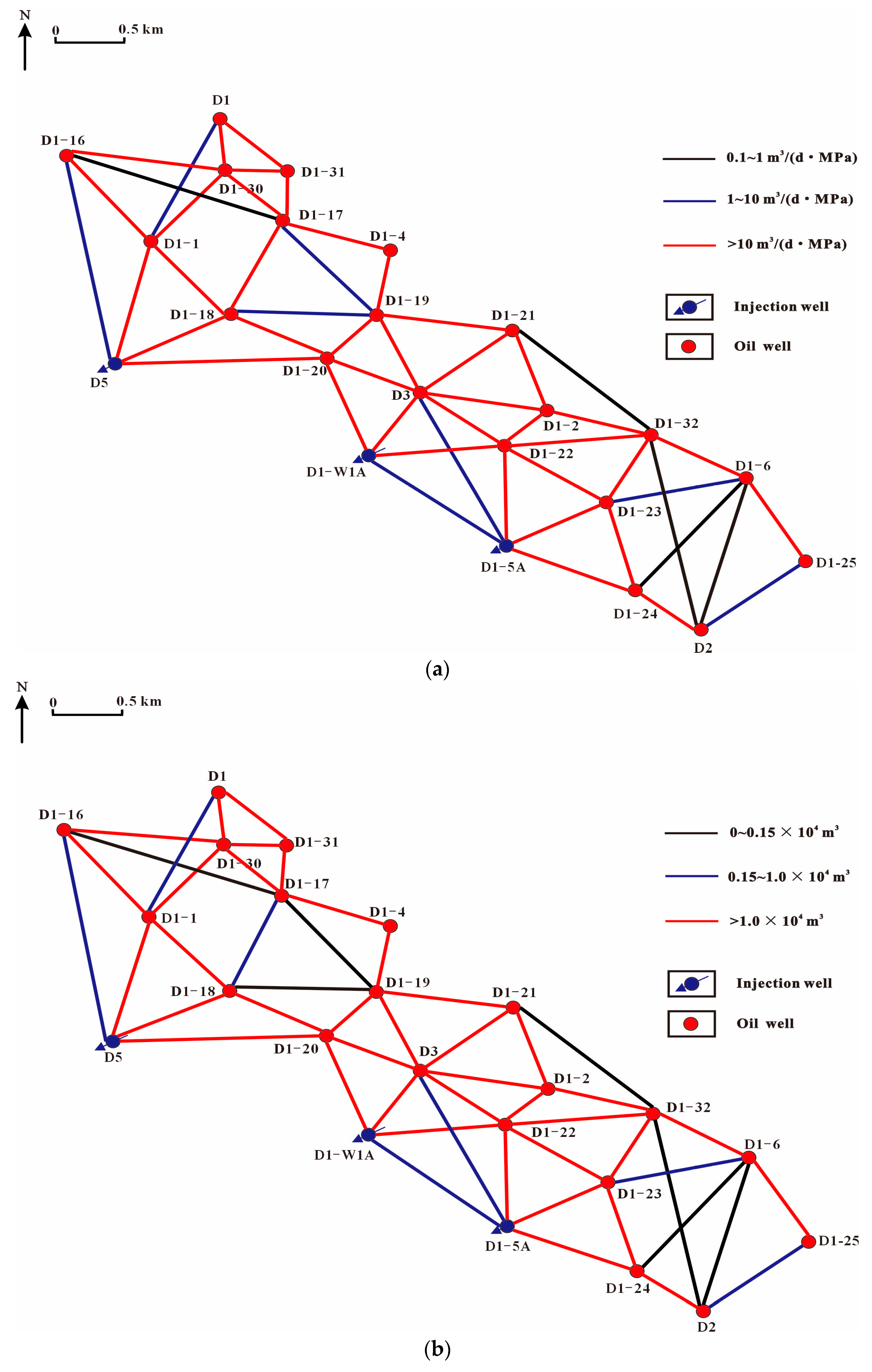
4.1. Model Validation

Based on the geological characteristic parameters of the reservoir and the actual production dynamic data, the historical production dynamic data of the block are used as the inversion index. By appropriately modifying the inter-well-connected volume and conductivity, the automatic history matching of the reservoir is realized, and accurate inversion results are obtained as shown in Figure 2.
To verify the accuracy of the inter-well connectivity model, the D1-5A well group is selected as an example, as shown in Figure 3.
The results of the splitting coefficient calculated by this model are compared with the actual field tracer water injection monitoring, as shown in Table 1 and Figure 4. The tracer response of the injection well D1-5A was mainly monitored in wells D1-23, D1-24, D1-22, and D3. The water flooding velocity in each direction can be inferred by the distance between the injection well and each production well and the effective time of tracer monitoring. At the same time, combined with the water injection splitting coefficient, it can be concluded that the fastest tracer monitoring response is that the water flooding speed of the D1-24 well is 84.2 m/d, and the water injection splitting coefficient is 31%, which is the highest among the four production wells. The second is well D1-23; the water flooding speed is 42.7 m/d, and the water injection splitting coefficient is 26%. The water injection splitting coefficient of well D1-22 and well D3 is consistent with the actual monitoring data of the tracer field. Among them, the tracer monitors the wells with faster water flooding speed, and the corresponding water injection splitting coefficient is larger, which fully verifies the accuracy of the model.

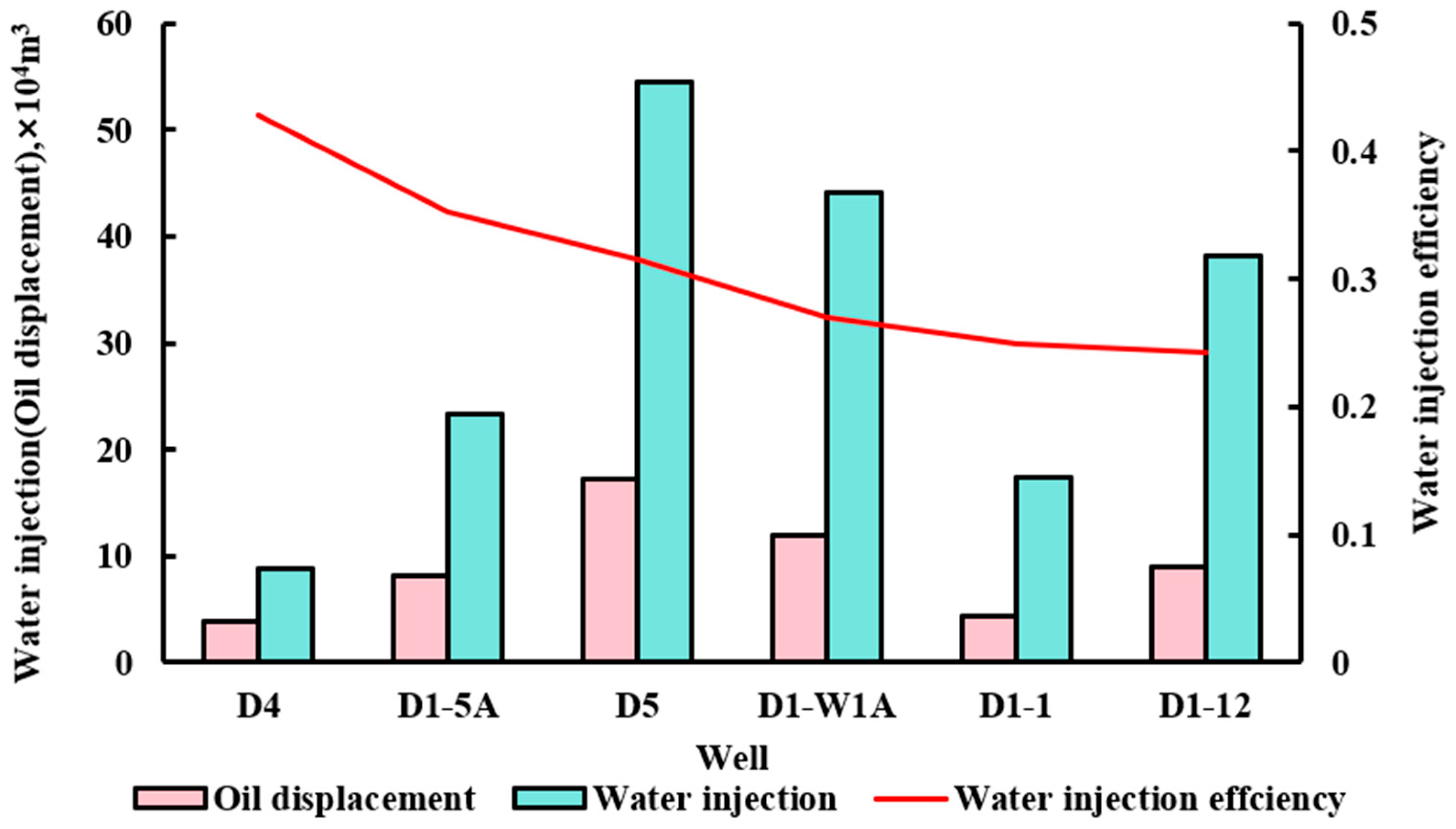
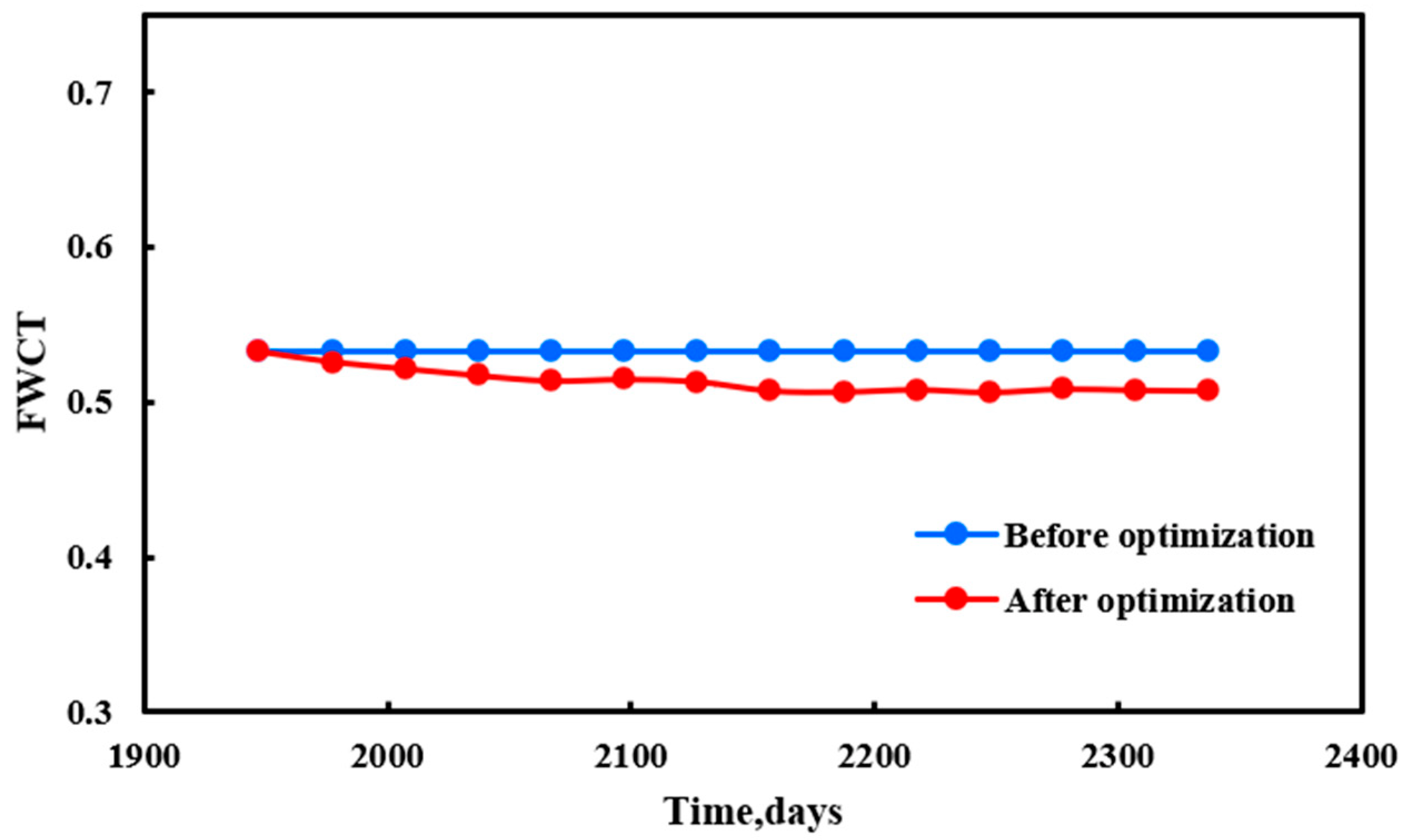
4.2. Production Optimization

The inter-well connectivity model can predict the production performance after obtaining a good historical fitting effect. By analyzing and calculating the cumulative liquid production, cumulative oil production, and cumulative water injection splitting coefficient of each oil well, the average water injection efficiency of the corresponding block is obtained. The water injection efficiency of each production well is statistically analyzed. When the water injection efficiency is lower than the average water injection efficiency of the current block, the water injection is reduced; otherwise, the water injection is increased. It is calculated that the average water injection efficiency of the current block is 31%. Therefore, when the water injection efficiency of the water injection well is lower than 31%, it is an inefficient well, and when it is higher than 31%, it is an efficient well. There are a total of six water injection wells in the study area, of which three are efficient and three are inefficient. As shown in Figure 5, the water injection efficiency is low for the entire block.
Based on the parameters of water injection efficiency of water injection wells, oil exchange rate of production wells, water cut of production wells, and injection–production efficiency of D reservoir in Chad oilfield, reasonable suggestions and measures are put forward for the adjustment of injection–production structure by using the connectivity relationship between wells and the characteristics of block development. According to the comparison of water injection efficiency, low-efficiency wells, and high-efficiency wells are judged, water injection volume is adjusted for high-efficiency and low-efficiency wells, water injection is reduced for low-efficiency wells, and water injection is increased for high-efficiency wells. At the same time, the water injection volume of water injection wells is optimized and adjusted in real time by combining the optimization algorithm. The actual water injection adjustment scheme of water injection wells is shown in Table 2.
According to the adjustment of production optimization, the cumulative oil production in the study area increased from 368 . 64 × 10 4 m3 to 370.27 × 10 4 m3, and the oil production increased by 1.63 × 10 4 m3. The moisture content decreased from 53.3% to 50.7%, a decrease of 2.6%, as shown in Figure 6 and Figure 7.

5. Conclusions

(1) Based on the theory of inter-well connectivity, a multi-layer sandstone reservoir model is established, and the reservoir dynamic parameter inversion and injection–production structure optimization were realized by using the optimization method.
(2) Based on the characteristic production and development parameters of the D reservoir in Chad, a multi-layer inter-well connectivity model was established. The inter-well conductivity and connectivity volume values were adjusted by field tracer data analysis, and the inter-well connectivity relationship field was obtained in real time. Through historical fitting calculation combined with tracer monitoring results, the fitting accuracy exceeded 94%, which fully verified the accuracy of the model.
(3) By using the cumulative liquid production of production wells and the cumulative splitting coefficient of water injection wells, the water injection efficiency was obtained. According to the water injection efficiency, the water injection wells were divided into inefficient wells and efficient wells. Combined with the optimization algorithm, the injection volume of water injection wells was optimized and controlled, and the injection–production optimization adjustment strategy was formulated. The strategy was applied to the Daniela reservoir in the Chad oilfield. After one year of production, the cumulative oil production in the study area increased by 1.3% per year, and the water cut decreased by 2.6%. The goal of increasing oil and controlling water was realized, which provides a reference for the formulation of the oilfield development plan.

Author Contributions

Conceptualization, Y.Z. and L.P.; methodology, Y.Z., S.D. and J.H.; validation, S.P., L.P. and Y.Z.; formal analysis, L.P. and S.D.; investigation, S.P., L.P. and Y.Z.; data curation, L.P. and J.H.; writing—original draft preparation, L.P.; writing—review and editing, Y.Z. and S.D.; visualization, S.P., L.P. and J.H.; funding acquisition, Y.Z. and L.P. and S.D. All authors have read and agreed to the published version of the manuscript.

Funding

This work was financially supported by the Natural Science Foundation of Xinjiang Uygur Autonomous Region (No. 2022D01A330) and the National Natural Science Foundation of China (No. 52274030) and the “Tianchi Talent” Introduction Plan of Xinjiang Uygur Autonomous Region (2022).

Data Availability Statement

The data that support the findings of this study are available from the corresponding author upon reasonable request.

Conflicts of Interest

The authors declare that the research was conducted in the absence of any commercial or financial relationships that could be construed as a potential conflict of interest.

References

  1. Wang, P.; Jiang, R.; Wang, G.; Ning, G. Numerical Simulation of Factors Affecting Water-flooding in High Water-cut Stage. Nat. Gas Oil 2012, 30, 36–38. [Google Scholar]
  2. Liu, W.; Liu, T.; Ji, Y.; Zhang, L.; Chu, F.; Zhang, L. Determination of inter-well connectivity of fractured fractures in glutenite reservoirs by micro-seismic monitoring results: A case study of Mahu Oilfield in the Junggar Basin. Oil Geophys. Prospect. 2022, 57, 395–404+246. [Google Scholar]
  3. Mirzayev, M.; Riazi, N.; Cronkwright, D.; Jensen, J.L.; Pedersen, P.K. Determining well-to-well connectivity using a modified capacitance model, seismic, and geology for a Bakken Waterflood. J. Pet. Sci. Eng. 2017, 152, 611–627. [Google Scholar] [CrossRef]
  4. Qu, C.; Liu, B.; Song, H.; Xie, T.; Zhang, Z. Inter well connectivity of reservoir after polymer flooding based on dynamic and static data coupling judgment method—By taking Bohai L oilfield as an example. Pet. Geol. Eng. 2021, 35, 76–79. [Google Scholar]
  5. Zhang, H.Y.; Zhou, X.; Wang, A.Q. Log Evaluation Method for Fractured-Vuggy Reservoir in the Dengying Formation of the Anyue Block, Sichuan Basin. Well Logging Technol. 2018, 42, 91–97. [Google Scholar]
  6. Patidar, A.K.; Joshi, D.; Dristant, U.; Choudhury, T. A review of tracer testing techniques in porous media specially attributed to the oil and gas industry. J. Pet. Explor. Prod. Technol. 2022, 12, 3339–3356. [Google Scholar] [CrossRef]
  7. Zhang, Y. Study on the Adjustment Strategy of the Horizontal Well Development in Bohai BZ Oilfield. Master’s Thesis, China University of Petroleum, Beijing, China, 2022. [Google Scholar] [CrossRef]
  8. Fang, X.; Yan, H.; Zhang, H.; Sun, X.; Peng, W. Dificulties and Technical Application of Complex Reservoir Modeling in West of South China Sea Oil and Gas Field. Offshore Oil 2016, 36, 50–55+98. [Google Scholar]
  9. Ye, X.; Huo, C.; Wang, P.; Xu, J.; Yang, J. A reservoir modeling method by comprehensive utilization of various data. Pet. Reserv. Eval. Dev. 2017, 7, 1–5. [Google Scholar] [CrossRef]
  10. Cao, X.; Wang, L.; Yu, Z. Application of Tracer Monitoring Technology in Reservoir Homogeneity and Reservoir Connectivity. Unconv. Oil Gas 2019, 6, 71–76. [Google Scholar]
  11. Chen, W.; Huang, B.; Gao, Y. The application of inter-well trace substance tracer technology in Suizhong 36-1 oilfield. Tianjin Sci. Technol. 2019, 36, 58–61. [Google Scholar]
  12. Yu, Q.; Liu, B.; Liu, C.; Zhang, X.; Zhang, X. Evaluation of inter-well dynamic connectivity based on polymer numerical simulation. Fault-Block Oil Gas Field 2017, 24, 827–830. [Google Scholar]
  13. Li, N.; Yang, L.; Zheng, X.; Zhang, J.; Liu, Y.; Ma, J. Evaluation on Injection-Production Connectivity of Low-Permeability Reservoirs Based on Tracer Monitoring and Numerical Simulation. Xinjiang Pet. Geol. 2021, 42, 735–740. [Google Scholar]
  14. Albertoni, A.; Lake, L.W. Inferring inter-well connectivity only from well-rate fluctuations in waterfloods. SPE Reserv. Eval. Eng. 2003, 6, 6–16. [Google Scholar] [CrossRef]
  15. Yousef, A.A.; Gentil, P.; Jensen, J.L.; Lake, L.W. A Capacitance Model to Infer Inter-well Connectivity from Production and Injection Rate Fluctuations. In Proceedings of the Presented at the SPE Annual Technical Conference and Exhibition, Dallas, TX, USA, 9–12 October 2005. [Google Scholar] [CrossRef]
  16. Sayarpour, M.; Kabir, C.S.; Sepehrnoori, K.; Lake, L.W. Probabilistic history matching with the capacitance-resistance model in waterfloods: A precursor to numerical modeling. In SPE Improved Oil Recovery Symposium; OnePetro: Richardson, TX, USA, 2010. [Google Scholar]
  17. Kaviani, D.; Valkó, P.P.; Jensen, J.L. Application of the multi-well productivity index-based method to evaluate inter-well connectivity. In SPE Improved Oil Recovery Symposium; OnePetro: Richardson, TX, USA, 2010. [Google Scholar]
  18. Liu, W.; Liu, W.; Gu, J.; Ji, C.; Sui, G. Research on inter-well connectivity of oil reservoirs based on Kalman filter and artificial neural network. Pet. Geol. Recovery Effic. 2020, 27, 118–124. [Google Scholar] [CrossRef]
  19. Zhao, H.; Kang, Z.; Zhang, X.; Sun, H.; Cao, L.; Reynolds, A.C. A physics-based data-driven numerical model for reservoir history matching and prediction with a field application. SPE J. 2016, 21, 2175–2194. [Google Scholar] [CrossRef]
  20. Zhao, H.; Xu, L.; Guo, Z.; Liu, W.; Zhang, Q.; Ning, X.; Li, G.; Shi, L. A new and fast waterflooding optimization workflow based on INSIM-derived injection efficiency with a field application. J. Pet. Sci. Eng. 2019, 179, 1186–1200. [Google Scholar] [CrossRef]
  21. Teng, X.; Li, Y.; Yang, P.; Yang, K.; Li, N.; Xie, E. Differential structural deformation and its control factors in the eastern segment of Kuqa depression. Pet. Geol. Recovery Effic. 2017, 24, 15–21. [Google Scholar]
  22. Dou, L.; Xiao, K.; Hu, Y.; Cheng, D.; Du, Y. Petroleum geology and a model of hydrocarbon accumulations in the Bongor Basin, the Republic of Chad. Acta Pet. Sin. 2011, 32, 379–386. [Google Scholar]
  23. Song, H.; Dou, L.; Xiao, K.; Hu, Y.; Ren, L. An exploratory research on geological conditions of hydrocarbon pooling and distribution patterns of reservoirs in the Bongor Basin. Oil Gas Geol. 2009, 30, 762–767. [Google Scholar]
  24. Zhao, H.; Zhang, X.; Wang, C.; He, H.; Xu, L.; Zhang, G.; Wang, S. Optimization of Fine water injection for reservoir stratification based on connectivity method. J. Yangtze Univ. 2018, 15, 42–51+6–7. [Google Scholar] [CrossRef]
  25. Zhao, H.; Kang, Z.; Zhang, Y.; Sun, H.; Li, Y. An inter-well connectivity numerical method for geological parameter characterization and oil-water two-phase dynamic prediction. Acta Pet. Sin. 2014, 35, 922. [Google Scholar]
  26. Guo, Z.; Reynolds, A.C.; Zhao, H. A physics-based data-driven model for history-matching, prediction and characterization of waterflooding performance. In SPE Reservoir Simulation Conference; OnePetro: Richardson, TX, USA, 2017. [Google Scholar]
  27. Zhao, H.; Xie, P.; Cao, L.; Li, Y.; Zhao, Y. Reservoir production optimization method based on inter-well connectivity. Acta Pet. Sin. 2017, 38, 555. [Google Scholar]
  28. Zhao, H.; Li, Y.; Cui, S.; Shang, G.; Reynolds, A.C.; Guo, Z.; Li, H.A. History matching and production optimization of water flooding based on a data-driven inter-well numerical simulation model. J. Nat. Gas Sci. Eng. 2016, 31, 48–66. [Google Scholar] [CrossRef]
  29. Zhao, H.; Cao, L.; Li, Y.; Yao, J. Production optimization of oil reservoirs based on an improved simultaneous perturbation stochastic approximation algorithm. Acta Pet. Sin. 2011, 32, 1031. [Google Scholar]
  30. Song, K.; Wu, Y.; Ji, B. A U-function method for estimating distribution of residual oil saturation in water drive reservoir. Acta Pet. Sin. 2006, 27, 91. [Google Scholar]
  31. Shen, W.; Zhao, H.; Liu, W.; Xu, L.; Liao, M. Identification method of dominant channeling in fractured vuggy carbonate reservoir based on connectivity model. Fault-Block Oil Gas Field 2018, 25, 459–463. [Google Scholar]
  32. Zhang, K.; Li, Y.; Yao, J.; Liu, J.; Yan, X. Theoretical research on production optimization of oil reservoirs. Acta Pet. Sin. 2010, 31, 78. [Google Scholar]
  33. Guo, Z.; Reynolds, A.C. INSIM-FT in three-dimensions with gravity. J. Comput. Phys. 2019, 380, 143–169. [Google Scholar] [CrossRef]
  34. Zhou, Y.; Lei, S.; Du, X.; Ju, S.; Li, W. Injection-production optimization of carbonate reservoir based on an inter-well connectivity model. Energy Explor. Exploit. 2021, 39, 1666–1684. [Google Scholar] [CrossRef]
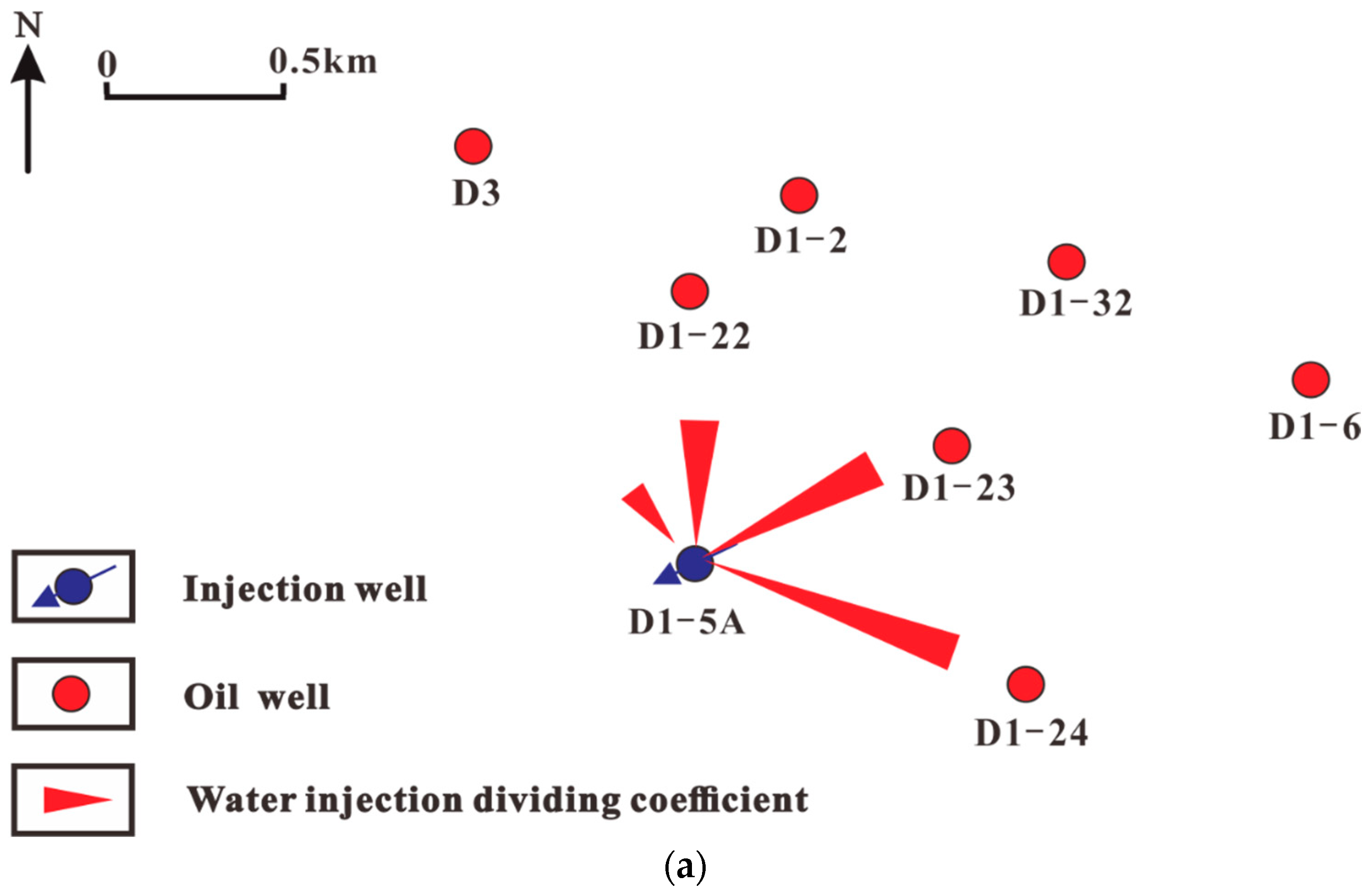
Figure 1. Regional tectonic location of Bongor basin.
Processes 11 02816 g001
Figure 2. (a) Transmissibility; (b) Connective volume.
Processes 11 02816 g002
Figure 3. Schematic diagram of well group and well location.
Processes 11 02816 g003
Figure 4. (a) Water injection dividing coefficient; (b) Tracer water flooding monitoring direction.
Processes 11 02816 g004aProcesses 11 02816 g004b
Figure 5. Water injection efficiency.
Processes 11 02816 g005
Figure 6. Before and after optimization in the study area of FOPT.
Processes 11 02816 g006
Figure 7. Before and after optimization in the study area of FWCT.
Processes 11 02816 g007
Table 1. Water injection splitting coefficient and tracer monitoring water flooding speed of D1-5A well group.
WellWell Spacing
/m
Water Drive Velocity/(M·d−1)Water Injection Dividing Coefficient
/%
D1-2485684.231
D1-2378962.726
D1-2284248.618
D3105926.313
Table 2. Adjustment strategy of injection–production structure in the study area.
WellOptimization MeasuresDaily Water Injection Rate/m3Water Injection Change Amount/(m3·d−1)
D4increase19922
D5increase9712
D1-1decrease4219
D1-12decrease12040
D1-5Aincrease14152
D1-W1Adecrease9131
Disclaimer/Publisher’s Note: The statements, opinions and data contained in all publications are solely those of the individual author(s) and contributor(s) and not of MDPI and/or the editor(s). MDPI and/or the editor(s) disclaim responsibility for any injury to people or property resulting from any ideas, methods, instructions or products referred to in the content.

