Abstract
This paper constructs a nonlinearly parametrized hypersonic cruise vehicle model on the basis of the existing on-orbit flight data using a curve-fitting technique. The hypersonic cruise vehicle system is separated into two interconnected subsystem: an attitude subsystem with rotational dynamics and a velocity subsystem with engine dynamics. The continuous adaptive controllers are designed for two subsystems using a novel function bounding technique and appropriate coordinate transformations, respectively, which ensure the global boundedness of all signals and achieve the non-zero equilibrium point regulation of nonlinearly parametrized hypersonic vehicle systems. One of the implications of this result is that growing nonlinearities in the uncertain model of the hypersonic vehicle system may be allowed for global stabilization. A simulation result verifies the effectiveness of the proposed adaptive control scheme.
1. Introduction
It has been known that hypersonic vehicle dynamic models are extremely complicated multivariate systems with serious nonlinearity, strong coupling, fast time-variability, and uncertainty, compared with the traditional air vehicle. These characteristics make the vehicle modeling and control research extremely scientific and challenging for the controlled hypersonic vehicles [1,2,3,4].
Hypersonic technique plays an important role in the future of military, political and economic development, since it has both the advantages of aviation technology and the incomparable advantages of spacecraft, which is used to cruise in the atmosphere and cross the atmosphere to re-orbit operation. As one typical application of the hypersonic technique, the research of hypersonic vehicles in modeling and control has attracted increasing attention over the last few decades [5,6,7,8,9,10]. In reference [5], for uncertain longitudinal dynamics of a hypersonic aircraft model, a nonlinear controller was designed using a robust sum-of-squares/robust linear matrix inequality method. In the literature [6], an adaptive sliding controller for the multi-input multi-output (MIMO) systems was proposed based on a variable structure control technique, which achieved the desired performance for the longitudinal dynamics of a generic hypersonic vehicle. When the actuator saturations, external disturbances or system faults appear in a hypersonic vehicle model, there are a lot of new control problems for control-oriented model of air-breathing hypersonic vehicles [7,8,9,10].
Fortunately, some difficult control issues have been researched to help to describe and understand these complexities and difficulties during the past years. These studies have mainly focused on velocity control and attitude control [11,12,13,14,15,16]. These references mainly considered the attitude and velocity tracking control problem for a longitudinal model of hypersonic vehicles. For an attitude dynamic model, based on the longitudinal model the references [11,15,16] discussed, the attitude control problem and the tracking control problem were mainly elaborated. In addition, many strategies have also been presented to design an appropriate controller for the longitudinal model with the flexible models. For example, for the longitudinal model using approximate linearization or the input–output feedback linearization based formulation, some traditional control design methods have also been used to construct the controller, including adaptive control, gain scheduling control and variable structure control, and so on [17,18,19]. It may be conceptually simple for the controller construction to meet certain objectives when the system dynamics are straightforward. With the persistent higher requirement for control objective and the better accuracy of control schemes, many existing methods are not effective enough to provide satisfactory performance when the longitudinal dynamics have severe uncertainties and undergo strong state coupling.
While these control methods succeed in solving many control problems, there is a common feature: the parameters in aerodynamic models are assumed to exist linearly in equations, that is, the controlled systems are linearly parametrized. However, aerodynamic models of real hypersonic vehicles have complicated structures and uncertain parameters, which cannot be linearly parametrized. The objective of this paper is to construct a nonlinearly parametrized aerodynamic model and develop an adaptive control scheme to address the following basic question:
If the longitudinal dynamic model of the hypersonic vehicles includes uncertain parameters and unknown functions with nonlinear parametrization, is it possible and how to design an adaptive state-feedback controller for the hypersonic vehicle system to achieve desired performance?
In order to seek a solution scheme to answer the aforementioned question, we introduce suitable transformations to convert the hypersonic vehicle control system to be investigated into a system with a strict-feedback form. Then, we propose a recursive procedure in designing an adaptive state-feedback controller based on a function bounding technique [20] and a backstepping method [21]. The designed controller guarantees global stability of the resulting closed-loop system. The main features and contributions of this paper are from three aspects:
- (i)
- Nonlinearly parametrized models are built by a curve-fitting technique according to aerodynamic data, which improve the accuracy of models and extends the scope of a nonlinear controlled object.
- (ii)
- An effective coordinate transformation and a new parameter separation technique are introduced to make the unknown parameters separate from the nonlinear dynamics.
- (iii)
- The adaptive backstepping control method improves the adaptability and robustness of the control algorithm, only requiring the structure of the upper-bound function bounding knowledge.
This paper is organized as follows. In Section 2, the hypersonic vehicle model is presented and the control objective is stated. In Section 3, the adaptive controllers are developed which ensure the closed-loop system global stability and achieve the hypersonic vehicle system adaptive regulation, where some preliminaries including several technical lemmas are also given. In Section 4, the simulation result verifies the effectiveness of the proposed adaptive control scheme. Finally, some conclusions are summarized in Section 5.
2. Modeling of Hypersonic Vehicle Model
The rigid-body dynamics of hypersonic vehicle studied in this paper is from [6], and we consider hypersonic cruising regimes and leave out ascent and reentry maneuvers. The longitudinal dynamic model of the hypersonic vehicle can be described by a set of differential equations as
The lift force T, drag force D, thrust force L and the pitching moment are modeled as follows [4]:
The nomenclatures are given in Table 1, where states are , control inputs are , and unknown parameters are and . Aerodynamic coefficients are smooth functions, which have the following expressions and and . Aerodynamic coefficients , and will be determined later. In what follows, suppose that all the state variables are available for feedback control design.

Table 1.
States, inputs and physical constants.
The real-life hypersonic vehicles have complex dynamics with high nonlinearity, strong coupling and fast time-varying. In addition, the complex flight environment results in the uncertain dynamics of a hypersonic vehicle system model. Those factors may result in the system dynamics unable to be linearly parametrized, that is, unknown system parameters only are represented in nonlinear functions. To obtain accurate expressions of the aerodynamic coefficients for the hypersonic vehicle, it needs to describe nonlinear function relationships between aerodynamic forces or aerodynamic moment and velocity V, angle of attack , pitch rate q, elevator angular deflection and engine throttle setting , based on the flight data of literature [22,23]. It needs be pointed out that the aerodynamic coefficients in the existing results are almost based on linearly parametrized expressions. Therefore, in this work, we give the nonlinearly parametrized analytic expressions of aerodynamic functions at velocity ft/s and height ft and two fitting indexes: sum of squares error (SSE) and coefficient of determination (R-square) by a data fitting curve technique. Our results are shown the drag coefficient during the cruise phase can be modeled as
whose SSE is 0.000199 and R-square is 0.9999. Similarly, the lift coefficient is
whose SSE is and R-square is 0.996. The contribution to moment due to angle of attack is
whose SSE is and R-square is 0.999.
Remark 1.
The SSE means a sum of the square of error between fitting data and original data. If an SSE is closer to 0, the selected function is more accurate and the data prediction is more successful. The R-square characterizes the accuracy of data fitting. If the R-square is closer to 1, the explanatory power of the coefficients is stronger and the fitting function is better. According to aforementioned data, we also fit linearly parametrized models of coefficients , and as follows: , and , and give the corresponding SSE and R-square, whose values of SSEs are , and and values of R-squares are 0.9970, 0.8454 and 0.9962, respectively. Therefore, nonlinear aerodynamic coefficients possess better modeling accuracy than linear aerodynamic coefficients.
To design state-feedback controllers for the nonlinear longitudinal model of the hypersonic vehicle, several clarifications about aerodynamic coefficients are addressed as follows:
- (i)
- Because the nonlinearly parametrized form of is sinusoidal, the coefficient can be approximate to a linear relation of in a small range value of .
- (ii)
- Considering the uncertainties of aerodynamic coefficients and developing the accuracy of curve fitting, we define the aerodynamic coefficients in (10)–(12) as the unknown aerodynamic coefficients, which can be expressed as
To design adaptive state-feedback controllers, the following assumptions and lemmas are used to obtain the hypersonic vehicle system with a strict-feedback form.
Assumption 1.
In (2), the term can be neglected since it is generally much smaller than lift L.
Assumption 2.
The speed change of the hypersonic vehicle is slow, and the variation range is small.
Remark 2.
From the literature [24,25], the value of is about two orders of magnitude smaller than the value of L in (2) during the cruise phase condition based on data by NASA report [1] and has low impact on the flight-path angle, which makes Assumption 1 reasonable.
Useful lemmas are applied in the controller design and stability analysis. Proofs of Lemmas 1 and 2 can be found in [21,26].
Lemma 1.
If and , then for any , there exists such that
Lemma 2.
For any real-valued continuous function where , there are smooth scalar value functions and such that
In this paper, our control objective is to concentrate on global adaptive control of the nonlinearly parametrized hypersonic vehicle system of the form (1)–(5) under Assumption 1 and Assumption 2. The designed continuous adaptive controllers make the closed-loop system stable in the sense of Lyapunov and achieve adaptive regulation.
3. Control Design and Stability Analysis
In this section, it is observed from Equations (1)–(9) that the rate change of attitude is mainly governed by the elevator deflection and the velocity is mainly controlled by the throttle setting . Therefore, we separate the longitudinal dynamics into two subsystems: an attitude subsystem with rotational dynamics and a velocity subsystem with engine dynamics. Then, we adopt the backstepping method and design adaptive controllers for two subsystems, separately.
3.1. The Attitude Subsystem Design
The purpose of this part is to explain and solve the adaptive regulation problem for the uncertain attitude subsystem with rotational dynamics (2)–(5) within a partial nonlinearly parametrized coefficient of aerodynamic force (15). A continuous adaptive state feedback controller can be explicitly constructed with the help of a backstepping control method and a parameter separation technique.
When the flight path angle varies between and , the Equation (3) shows that a nonlinear mapping between the height h and the flight path angle is an one-to-one relationship, that is, when the flight path angle regulates a steady state value during the cruise phase, the height h also achieves the corresponding value. Therefore, we consider the adaptive regulation problem of the --q subsystem (2), (4) and (5) instead of the attitude subsystem (2)–(5) in the procedure of control design.
For the attitude subsystem, we summarize the following theorem.
Theorem 1.
For the uncertain attitude subsystem (2)–(5) with partial nonlinear parametrization of the type (6)–(15), the following continuous adaptive state-feedback controller,
where with the pitch angle , and , is a continuous function, and is the on-line estimate of unknown parameter Ψ determined later, achieves the adaptive regulation problem with global stability of the closed-loop system.
Proof.
To apply the backstepping control method to the attitude subsystem (--q subsystem) subsystem (2), (4) and (5), we first formulate the attitude subsystem (--q subsystem) into a strict-feedback form. □
According to Assumption 1 and (13), the Equation (2) can be transformed into
where and is a continuous function.
From (4), the kinematic model of the pitch angle is transformed into
Similarly, in view of (9) and (15), the dynamic model (5) of the pitch rate can be rewritten as
where , and is a continuous function of nonlinear parameterization.
From the above definitions, we obtain the longitudinal model of a hypersonic vehicle as the strict feedback form
We know that and are just functions of the velocity V. It follows from Assumption 2 that
According to admissible ranges for system states in [27], there exist positive constants such that and satisfy the following inequalities
where represents the uncertainty.
To achieve the desired objective, we introduce the coordinate transformation
With (24), the system (21)–(23) can be transformed into the following form
where is a continuous function of with nonlinear parameterization and is a nonzero unknown bounded function.
The left proof is based on an inductive argument, which simultaneously constructs a Lyapunov function and designs a continuous adaptive state feedback controller for system (29)–(31). It is divided into two parts.
Part I: the procedure of adaptive controllers
First, inequality (25) ensures
where and are unknown bounded constants.
Since is a continuous function, it deduces from Lemma 2 that
where is a smooth function without unknown uncertainties, is an unknown upper bound of , and is an unknown constant.
Define
which is an unknown bounded constant in admissible ranges [27]. Using the backstepping method, we explicitly construct an alternative Lyapunov function and a one-dimensional adaptive controller for the nonlinearly parameterized system with respect to the new unknown parameter . This designed adaptive controller applied to the uncertain altitude subsystem (2)–(5) can solve the adaptive regulation problem.
Initial Step: Define with and where is the estimate error. Choose the Lyapunov function
which is apparently positive and proper. The derivation of along the trajectories of (29) is given by
where is a virtual control signal. Choosing the virtual control signal , the Equation (36) can be expressed as
where is a state error and is a design parameter.
Second Step: Choose the Lyapunov function
Then, with (37) and Lemma 1, the time derivative of along the solutions of (30) is
where is a design parameter and is a constant.
Selecting a virtual control signal and defining a state error , we have
Third Step: We construct the positive and proper Lyapunov function
From (32), (40) and the fact that for with , we know that the time derivative of along the solutions of (31) is
Next, to design a suitable actual controller , it needs to estimate the last three terms on the right-hand side of (42) appropriately.
Due to the equality and the definitions of , one easily deduces
From Lemma 1, with the aid of (34), (43) and the definition of , we have
where is a known constant.
It follows from Lemma 1, the definition of , (43) and that
where are known constants.
With Lemma 1, we have
Substituting (44)–(46) into (42), we have
From (47), we choose an adaptive control law
and a controller
such that
where are design parameters.
Part II: stability analysis of the closed-loop system
By the existence and the continuity of solutions, the closed-loop system states composed of are defined with . From (35), (38), (41), we know where , as the function of , is positive definite and radially unbounded. From [28], there is a function such that
where . Similarly, there exists a function such that
Together with (51), we have
where is the state of the closed-loop system.
For any , noting that , one always finds a satisfying , such that . Because of the fact that , we have
where is the initial state. According to (53), if , we have
From (55), it deduces . Due to , we obtain
With the coordinate transformation (43) and the boundedness of , it is easy to obtain the boundedness of for .
From (54), the boundedness of and continuity of , we know that exists and is finite. Together with (50), we have
On the other hand, noting (29)–(31), (43), (49), (56) and the boundedness of , we know that is bounded. Thus, is uniformly continuous in t, so is , for . Then, using Barbalat’s Lemma in [28], we obtain , which in turn shows that . It follows from (43) that for .
From (26)–(28), we have
From Assumption 2, (21) and (58), we obtain
Therefore, we have
where is the equilibrium point during the cruise phase.
Up to now, we have achieved the adaptive regulation of the closed-loop systems with the designed controller (49) and the adaptive law (48). ∇
3.2. The Velocity Subsystem Design
In this section, we will design a continuous state-feedback controller for the velocity subsystem to regulate the vehicle velocity with the engine throttle .
For the velocity subsystem (1), we conclude the following theorem.
Theorem 2.
For the uncertain velocity subsystem (1), a following designed adaptive state-feedback controller,
where , with being a desired velocity, is a continuous function, and is an on-line estimate of unknown parameter Θ, which is determined later, solves the adaptive regulation problem with the global stability of the closed-loop system.
Proof.
The Equation (1) is rewritten as
where
where is a bounded uncertainty for a given constant . □
Note that is a function of system states V and . According to admissible ranges for system states in [27], there exist positive constants such that satisfies the following inequality
where represents the uncertainty.
Because is a smooth function, it deduces from Lemma 1 that
where is a continuous function without uncertainties, is an unknown upper bound of , and being an unknown constant.
On the basis of (67) and (68), we define
Now, we are ready to design a controller for the velocity subsystem (64) with respect to the new unknown parameter using the candidate Lyapunov function.
Consider the candidate Lyapunov function
which is positive definite and proper, where being a parameter error and is the estimate of .
Using (67)–(69) and the fact that , the derivation of W along the trajectories of (64) is given by
where is a known parameter.
According to (71), choosing the adaptive law
and the controller
renders
The stability analysis of the velocity subsystem with the adaptive controller (72) and (73) is similar to that of Theorem 1, and is omitted here. ∇
Remark 3.
For the adaptive control design, large gains , may lead to large control magnitude of defined in (49) and defined in (73), so the design parameters are suitably selected to avoid the rapid change of control inputs. For the robust adaptive control design, the gains , are suitably selected based on some trade-off of convergence rate and steady state error.
4. Simulation Results
In this section, we use simulation results to verify the effectiveness of our adaptive control schemes for the attitude subsystem (21)–(23) and the velocity subsystem (64).
4.1. Simulation Systems
According to the literature [29,30], model parameters of the hypersonic vehicle are given as , , , , and . All the parameters of the refined hypersonic vehicle system are listed as follows:
The trim condition of the nonlinearly parametrized hypersonic vehicle system (21)–(23) and (64) during a cruise phase is given as , , , , , .
4.2. Simulation Results
In this subsection, for the attitude subsystem (21)–(23) and the velocity subsystem (64), the controllers and are designed as
and the parameter update laws and are chosen as
where and are the determined continuous functions in Section 3.
If the initial condition of the closed-loop system is chosen as and , one can obtain Figure 1, Figure 2, Figure 3, Figure 4, Figure 5 and Figure 6. Four states are shown in Figure 1 and Figure 2 and two control inputs are shown in Figure 3 and Figure 4, where the blue lines mean the responses of states and inputs of the hypersonic vehicle and the red lines mean the control accuracy in the stable phase, which indicate that the designed controllers regulate the states of the hypersonic vehicle to the equilibrium point . Two parameter estimates are shown in Figure 5 and Figure 6, which indicate parameter estimates are the desired bounded functions.
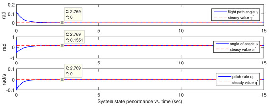
Figure 1.
The state responses of the altitude subsystem.
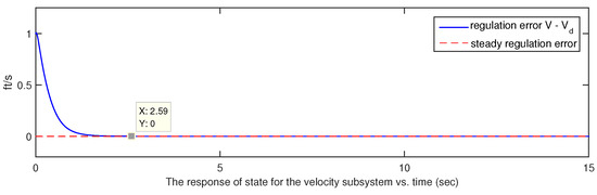
Figure 2.
The state error response of the velocity subsystem.
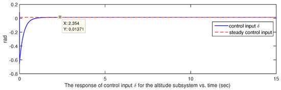
Figure 3.
The control input response of the altitude subsystem.
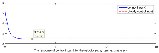
Figure 4.
The control input response of the velocity subsystem.
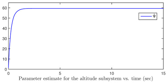
Figure 5.
The parameter estimate response of the altitude subsystem.
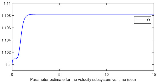
Figure 6.
The parameter estimate response of the velocity subsystem.
5. Conclusions
In this paper, we build nonlinearly parametrized rigid-body vehicle dynamics of a hypersonic vehicle and propose an adaptive control scheme combining a parameter separation technique and a backstepping method, which achieves a global stability of a nonlinearly parametrized hypersonic vehicle. Other adaptive control problems currently under investigation include a disturbance rejection and noise cancellation problem based on the proposed adaptive control schemes and the state feedback output tracking problem for a general multivariable system with nonlinear parametrization.
Author Contributions
Conceptualization, S.Y.; methodology, S.Y. and X.L.; software, X.L.; validation, S.Y. and X.L.; formal analysis, S.Y. and X.L.; writing—original draft preparation, S.Y.; writing—review and editing, S.Y.; supervision, S.Y.; project administration, S.Y.; funding acquisition, S.Y. All authors have read and agreed to the published version of the manuscript.
Funding
This research was funded by Natural Science Foundation of Shandong Province of China, grant number ZR2022QF021.
Data Availability Statement
Not applicable.
Conflicts of Interest
The authors declare no conflict of interest.
References
- Freeman, D.C.; Reubush, D.E.; McClinton, C.R.; Rausch, V.L.; Crawford, J.L. The NASA Hyper-X program. In Proceedings of the 48th International Astronautical Congress, Paris, France, 6–10 October 1997. [Google Scholar]
- Hueter, U.; McClinton, C.R. NASA’s advanced space transportation hypersonic program. In Proceedings of the 11th AIAA/AAAF International Conference, Orleans, France, 29 September–4 October 2002; pp. 2002–5175. [Google Scholar]
- Davidson, J.; Lallman, F.J.; McMinn, J.D.; Martin, J.; Pahle, J.; Stephenson, M.; Selmon, J.; Bose, D. Flight control laws for NASA’s Hyper-X research vehicle. In Guidance, Navigation, and Control Conference and Exhibit; AIAA: Reston, VA, USA, 1999; pp. 99–4124. [Google Scholar]
- Fidan, B.; Mirmirani, M.; Ioannou, P. Flight dynamics and control of air-breathing hypersonic vehicles: Review and new directions. In AIAA International Space Planes and Hypersonic Systems and Technologies; AIAA: Reston, VA, USA, 2023; pp. 2003–7081. [Google Scholar]
- Ataei, A.; Wang, Q. Nonlinear control of an uncertain hypersonic aircraft model using robust sum-of-squares method. IET Control Theory Appl. 2012, 6, 203–215. [Google Scholar] [CrossRef]
- Xu, H.; Mirmirani, M.; Ioannou, P. Adaptive sliding mode control design for a hypersonic flight vehicle. J. Guid. Control Dyn. 2004, 27, 82–838. [Google Scholar] [CrossRef]
- Xu, B.; Huang, X.; Wang, D.; Sun, F. Dynamic surface control of constrained hypersonic flight models with parameter estimation and actuator compensation. Asian J. Control 2014, 16, 162–174. [Google Scholar] [CrossRef]
- Wilcox, Z.D.; Mackunis, W.; Bhat, S.; Lind, R.; Dixon, W.E. Robust nonlinear control of a hypersonic aircraft in the presence of aerothermoelastic effects. In Proceedings of the IEEE American Control Conference, St. Louis, MO, USA, 10–12 June 2009; pp. 2533–2538. [Google Scholar]
- Ren, W.; Jiang, B.; Yang, H. Singular perturbation-based fault-tolerant control of the air-breathing hypersonic vehicle. IEEE/ASME Trans. Mechatron. 2019, 24, 2562–2571. [Google Scholar] [CrossRef]
- Jiang, B.; Gao, Z.; Shi, P.; Xu, Y. Adaptive fault-tolerant tracking control of near-space vehicle using takagi–sugeno fuzzy models. IEEE Trans. Fuzzy Syst. 2010, 18, 1000–1007. [Google Scholar] [CrossRef]
- Gao, Z.; Jiang, B.; Shi, P.; Xu, Y. Fault-tolerant control for a near space vehicle with a stuck actuator fault based on a Takagi-Sugeno fuzzy model. Proc. IMechE Part I J. Syst. Control Eng. 2010, 224, 587–598. [Google Scholar] [CrossRef]
- Gibson, T.E.; Crespo, L.; Annaswamy, A.M. Adaptive control of hypersonic vehicles in the presence of modeling uncertainties. In Proceedings of the American Control Conference, St. Louis, MO, USA, 10–12 June 2009; pp. 3178–3183. [Google Scholar]
- Wang, Q.; Stengel, R.F. Robust nonlinear control of a hypersonic vehicle. J. Guid. Control Dyn. 2000, 23, 577–585. [Google Scholar] [CrossRef]
- Li, H.F.; Sun, W.C.; Li, Z.Y. Index approach law based sliding control for a hypersonic aircraft. In Proceedings of the International Symposium on Systems and Control in Aerospace and Astronautics, Shenzhen, China, 10–12 December 2008; pp. 1–5. [Google Scholar]
- Da, R.R.; Chu, Q.P.; Mulder, J.A. Reentry flight controller design using nonlinear dynamical inversion. J. Space Rocket 2003, 40, 64–71. [Google Scholar]
- Fiorentini, L.; Serrani, A. Adaptive restricted trajectory tracking for a non-minimum phase hypersonic vehicle model. Automatica 2012, 48, 1248–1261. [Google Scholar] [CrossRef]
- Cui, R.; Xie, X.J. Adaptive state-feedback stabilization of state-constrained stochastic high-order nonlinear systems. Sci. China Inf. Sci. 2021, 64, 10. [Google Scholar] [CrossRef]
- Li, G.; Xie, X.J. Adaptive state-feedback stabilization of stochastic high-order nonlinear systems with time-varying powers and stochastic inverse dynamics. IEEE Trans. Autom. Control 2022, 66, 5360–5367. [Google Scholar] [CrossRef]
- Cui, R.; Xie, X.J. Finite-time stabilization of output-constrained stochastic high-order nonlinear systems with high-order and low-order nonlinearities. Automatica 2022, 136, 110085. [Google Scholar] [CrossRef]
- Yang, S.H.; Tao, G.; Jiang, B.; Zhen, Z.Z. Practical output tracking control for nonlinearly parameterized longitudinal dynamics of air-breathing hypersonic vehicles. J. Frankl. Inst. 2020, 357, 12380–12413. [Google Scholar] [CrossRef]
- Lin, W.; Qian, C. Adaptive control of nonlinearly parameterized systems: The smooth feedback case. IEEE Trans. Autom. Control 2002, 47, 1249–1266. [Google Scholar] [CrossRef]
- Aerodynamic Design Data Book; Volume 1M Orbiter Vehicle STS-1; NASA Report; NASA: Washington, DC, USA, 1980.
- Shaughnessy, J.; Pinckney, S.; Mcminn, J.; Cruz, C.; Kelley, M. Hypersonic Vehicle Simulation Model: Winged-Cone Configuration; TM-102610; NASA: Washington, DC, USA, 1990.
- Gao, D.; Sun, Z.; Luo, X.; Du, T. Fuzzy adaptive control for hypersonic vehicle via backstepping method. Control Theory Appl. 2008, 25, 805–810. [Google Scholar]
- Xu, B.; Gao, D.; Wang, S. Adaptive neural control based on HGO for hypersonic flight vehicles. Sci. China Inf. Sci. 2011, 54, 511–520. [Google Scholar] [CrossRef]
- Cui, R.; Xie, X.J. Output feedback stabilization of stochastic planar nonlinear systems with output constraint. Automatica 2022, 143, 110471. [Google Scholar] [CrossRef]
- Fiorentini, L.; Serrani, A.; Bolender, M.A.; Doman, D.B. Nonlinear control of non-minimum phase hypersonic vehicle models. In Proceedings of the American Control Conference, St. Louis, MO, USA, 10–12 June 2009; pp. 3160–3165. [Google Scholar]
- Khalil, H. Nonlinear Systems; Prentice Hall: Hoboken, NJ, USA, 2002. [Google Scholar]
- Bolender, M.A.; Doman, D.B. A nonlinear longitudinal dynamical model of an air-breathing hypersonic vehicle. J. Spacecr. Rocket. 2007, 44, 374–387. [Google Scholar] [CrossRef]
- Yang, S.; Tao, G.; Jiang, B. Robust adaptive control of nonlinearly parametrized multivariable systems with unmatched disturbances. Int. J. Robust Nonlinear Control 2020, 30, 3582–3606. [Google Scholar] [CrossRef]
Disclaimer/Publisher’s Note: The statements, opinions and data contained in all publications are solely those of the individual author(s) and contributor(s) and not of MDPI and/or the editor(s). MDPI and/or the editor(s) disclaim responsibility for any injury to people or property resulting from any ideas, methods, instructions or products referred to in the content. |
© 2023 by the authors. Licensee MDPI, Basel, Switzerland. This article is an open access article distributed under the terms and conditions of the Creative Commons Attribution (CC BY) license (https://creativecommons.org/licenses/by/4.0/).