A Spark Streaming-Based Early Warning Model for Gas Concentration Prediction

Abstract

The prediction and early warning efficiency of mine gas concentrations are important for intelligent monitoring of daily gas concentrations in coal mines. It is used as an important means for ensuring the safe and stable operation of coal mines. This study proposes an early warning model for gas concentration prediction involving the Spark Streaming framework (SSF). The model incorporates a particle swarm optimisation algorithm (PSO) and a gated recurrent unit (GRU) model in the SSF, and further experimental analysis is carried out on the basis of optimising the model parameters. The operational efficiency of the model is validated using a control variable approach, and the prediction and warning errors is verified using MAE, RMSE and R². The results show that the model is able to predict and warn of the gas concentration with high efficiency and high accuracy. It also features fast data processing and fault tolerance, which provides a new idea to continue improving the gas concentration prediction and warning efficiency and some theoretical and technical support for intelligent gas monitoring in coal mines.

1. Introduction

Coal occupies a very important position in China’s energy structure, and safety is a necessary prerequisite for coal mining to ensure the economic efficiency of coal mines and the health of underground workers [1,2,3,4,5]. With the development of intelligent coal mines, accurate and efficient data mining has become an inevitable prerequisite for intelligent analysis and decision making, including the analysis and mining of gas concentration data. In recent years, as coal mining operations continue to expand much deeper, the underground operating environment has become increasingly complex, and gas hazards have become increasingly prominent [6,7,8,9]. At this stage, gas data monitoring technology has gradually matured, realising real-time online monitoring and real-time transmission and enabling online analysis and prediction based on various prediction models. A great deal of work has also been done in the field of gas prediction and early warning by domestic and international researchers through the use of algorithms, such as long short-term memory (LSTM), the autoregressive integrated moving average (ARIMA) model and support vector machines (SVMs) for gas concentration prediction [10,11,12,13,14]. An LSTM recurrent neural network prediction method is proposed for a gas concentration prediction analysis with prediction errors of 0.0005–0.04, demonstrating the applicability of the model for gas concentration prediction [15]. A combination of the autoregressive moving average (ARMA) model, the chaos time series (CHAOS) model, the ED model (single-sensor) and the ED model (multisensor) is proposed, which can predict gas concentrations at five different time steps with few errors, further improving the prediction accuracy [16]. A gated recursive unit (GRU)-based mine gas concentration prediction model is proposed, which can make full use of the time series characteristics of mine gas concentration data, and the prediction results have less errors and high practical value [17]. The random forest, extreme random regression tree and gradient boosted decision tree (selected GBDT) regression algorithms are used as base learning devices, and the output of each base learner is used as input using a superposition algorithm to train a new model for predicting gas concentrations. The results show that the superposition model had high prediction accuracy [18]. A self-recurrent wavelet neural network (SRWNN) based on interval prediction rather than point prediction is proposed as a prediction model, which is applicable to the gas concentration prediction system of large-scale intelligent edge devices and is better for gas concentration prediction analysis [19].

Since gas concentration data have strong time series characteristics [20,21], the algorithms in the above studies are able to predict gas concentration well, but most of the above studies focus on the accuracy of data prediction, and the prediction efficiency is mostly dependent on the operation efficiency of the model itself, which actually has certain limitations for improving the prediction efficiency. In this paper, we propose a gas concentration prediction model incorporating the particle swarm optimisation algorithm (PSO) and a gated recurrent unit (GRU) model under the Spark Streaming framework (SSF), which can further improve the model’s operational efficiency due to the advantages of fast data processing and fault tolerance of the SSF. The overlay model has the advantages of high convergence speed and high accuracy, which enables this superimposed model to complete the data analysis and mining with high efficiency and accuracy to achieve the real sense of real-time online analysis. This provides a new way of thinking for intelligent gas prediction and early warning, as well as some theoretical and technical support, which is of great importance to the intelligent construction of coal mines.

2. Materials and Methods

2.1. Spark Streaming

Spark Streaming is a distributed stream computing data processing framework based on the D Stream model, which allows batch processing of data in a short period of time, with the advantages of fast processing speed and fault tolerance [22,23,24]. D streams are part of the SSF and are composed of sequences of successive resilient distributed datasets (RDDs). The SSF essentially divides the collected data into individual D Streams and converts each D Stream into an RDD to be stored in memory and, eventually, to an external device.

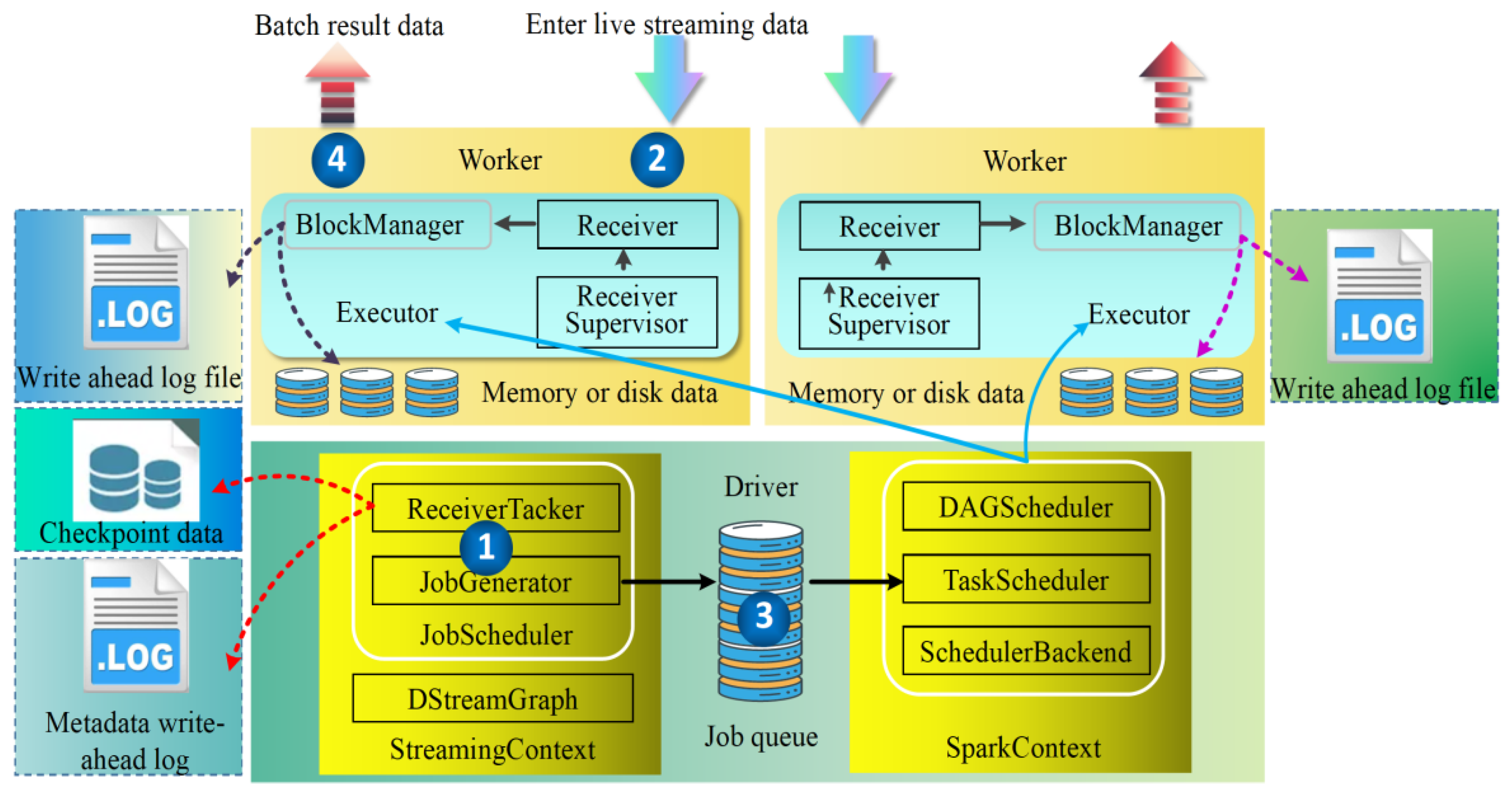
Spark Streaming for stream data processing can be roughly divided into four steps: starting the stream processing engine, receiving and storing stream data, processing stream data and outputting processing results. Its operation architecture is shown in Figure 1, initializing the streaming context object, instantiating the D Stream graph and job scheduler during the start-up of this object. The D Stream graph is used to store information such as D Streams and the dependencies between D Streams. Job scheduler includes receiver tracker and job generator. The receiver tracker is the manager of the driver-side stream data receiver, and the job generator is the batch job generator. During the start of the receiver tracker, the receiver supervisor in the corresponding executor is notified of the start of the stream data receiver according to the stream data receiver distribution policy, and then, the receiver supervisor starts the stream data receiver. The receiver is started, and it continuously receives real-time streaming data and makes a judgement based on the size of the data coming through. If the amount of data is small, multiple pieces of data are saved into one and then stored in blocks; if the amount of data is large, it is directly stored in blocks. Block storage is divided into two types depending on whether prewritten logging is set up: one type is to use the non-prewritten logging block manager-based block handler method to write directly to the worker’s memory or disk, and the other type is the write ahead log-based block handler method, which writes data to the worker’s memory or disk at the same time as prewriting the log. After the data are stored, the receiver supervisor reports the meta-information about the data storage to the receiver tracker, which then forwards this information to the receiver block tracker. The receiver block tracker is responsible for managing the meta-information about the received data blocks. A timer is maintained in streaming context’s job generator, which performs the job generation operation when the batch time arrives. As the data from the live stream continue to flow in, the Spark framework keeps processing the data and outputting the results accordingly.

2.2. Real-Time Predictive Early Warning SSPG Model Construction

The SSPG model is a PSO-GRU model combined with the SSF for the real-time prediction of gas concentrations. The PSO model is an evolutionary computational technique derived from the study of the predatory behaviour of bird populations, which has a faster convergence rate and better meets the requirements of the algorithm for real-time prediction. The mathematical idea is that, in an n-dimensional space S ∈ Rⁿ, each population consists of m particles, where the position of each particle i is x_i = (x_i1, x_i2, L, x_in), the velocity is v_i = (v_i1, v_i2, L, v_in) and the optimal position of each particle is p_i = (p_i1, p_i2, L, p_in). The optimal position of the whole particle population is p = (p_g1, p_g2, L, p_gn). Each particle velocity and position update equation are shown in Equations (1) and (2) [25,26,27].

$$v_i\left(t+1\right)=\omega v_i\left(t\right)+c_1{r}_1\left(t\right)\left[p_i\left(t\right)-x_i\left(t\right)\right]+c_2{r}_2\left(t\right)\left[p_g\left(t\right)-x_i\left(t\right)\right]$$

(1)

$$x_i\left(t+1\right)=x_i\left(t\right)+v_i\left(t+1\right)$$

(2)

where I = 1, 2, L, m, c₁ and c₂ are learning factors, r₁ and r₂ are random numbers within [0–1], t is the time and ω is the inertia weight; the larger ω is, the stronger the global search performance.

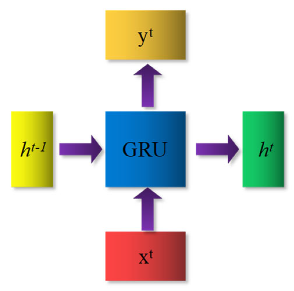
The GRU model is a commonly used gated recurrent neural network [28]. The GUR has two gates, a reset gate and an update gate. The reset gate determines how to combine the new input with the previous memory, and the update gate determines how much of the previous memory comes into play. There is a current input x^t and a hidden state h^t−1 passed down from the previous node. When combining x^t and h^t−1, the GRU obtains the output y^t of the current hidden point and the hidden state h^t passed down to the next node (Figure 2). 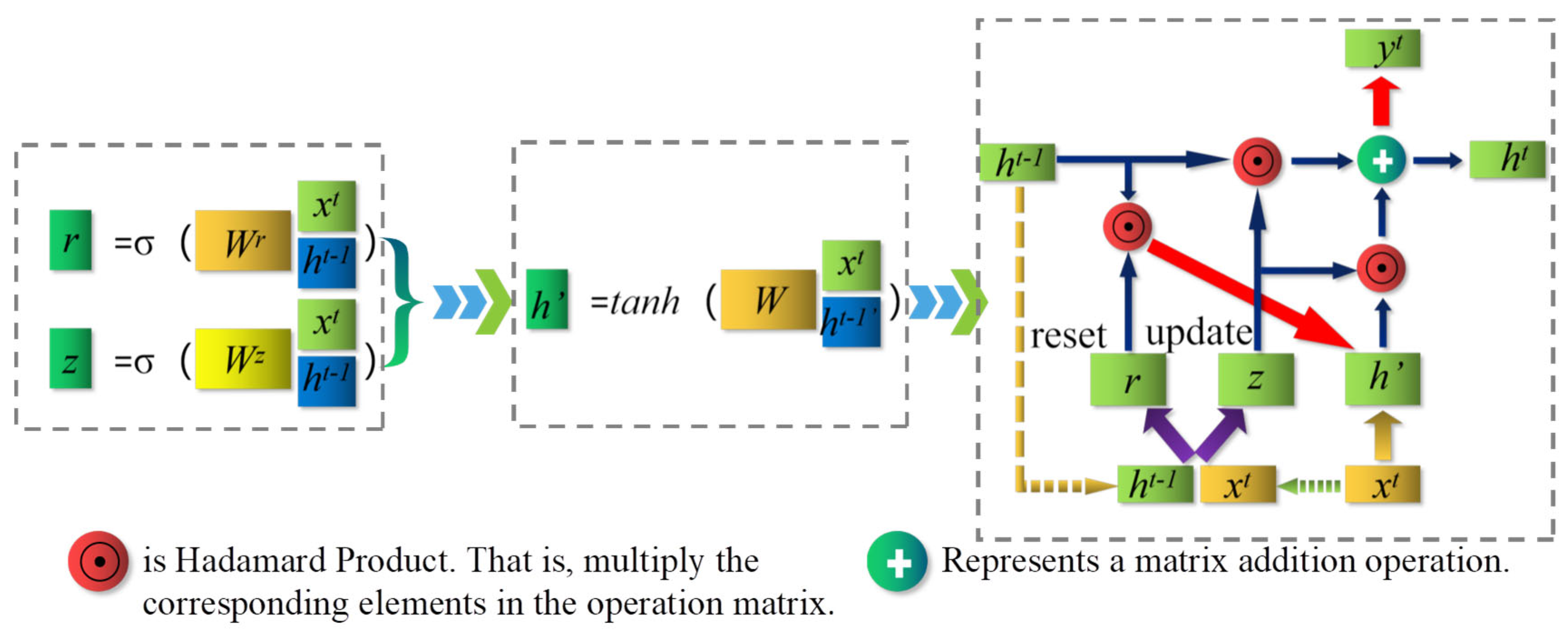The internal structure of the GRU is shown in Figure 3. r is the reset gate (see Equation (3)), z is the update gate (See Equation (4)), h^t is the hidden layer (see Equation (5)) and σ is the sigmoid function through which the data can be transformed to a value in the range of [0~1] to act as a gate signal. After obtaining the gating signal, we use reset gating to obtain the data h^t−1’ = h^t−1⊙r, then splice h^t−1’ with the input x^t and, in pass, as a tanh activation function to deflate the data to a range of [−1~1] to obtain h’ in Figure 3. h’ contains mainly the currently entered x^t data. The GRU has certain advantages in dealing with long time series data, such as the gas concentration [29]. The model can be divided into three parts: the input layer, hidden layer and output layer. The input layer is mainly used for pre-processing the original data and dividing the dataset, the hidden layer is used for optimising the parameters of the model with the minimum loss value as the evaluation index and the output layer is used for predicting the gas concentration according to the specific optimisation of the hidden layer [30].

$$r=\sigma (W^r{x}^t+U^r{h}^{t-1})$$

(3)

$$z=\sigma (W^z{x}^t+U^z{h}^{t-1})$$

(4)

$$h^t=(1-z^t)h^{t-1}+z^t$$

(5)

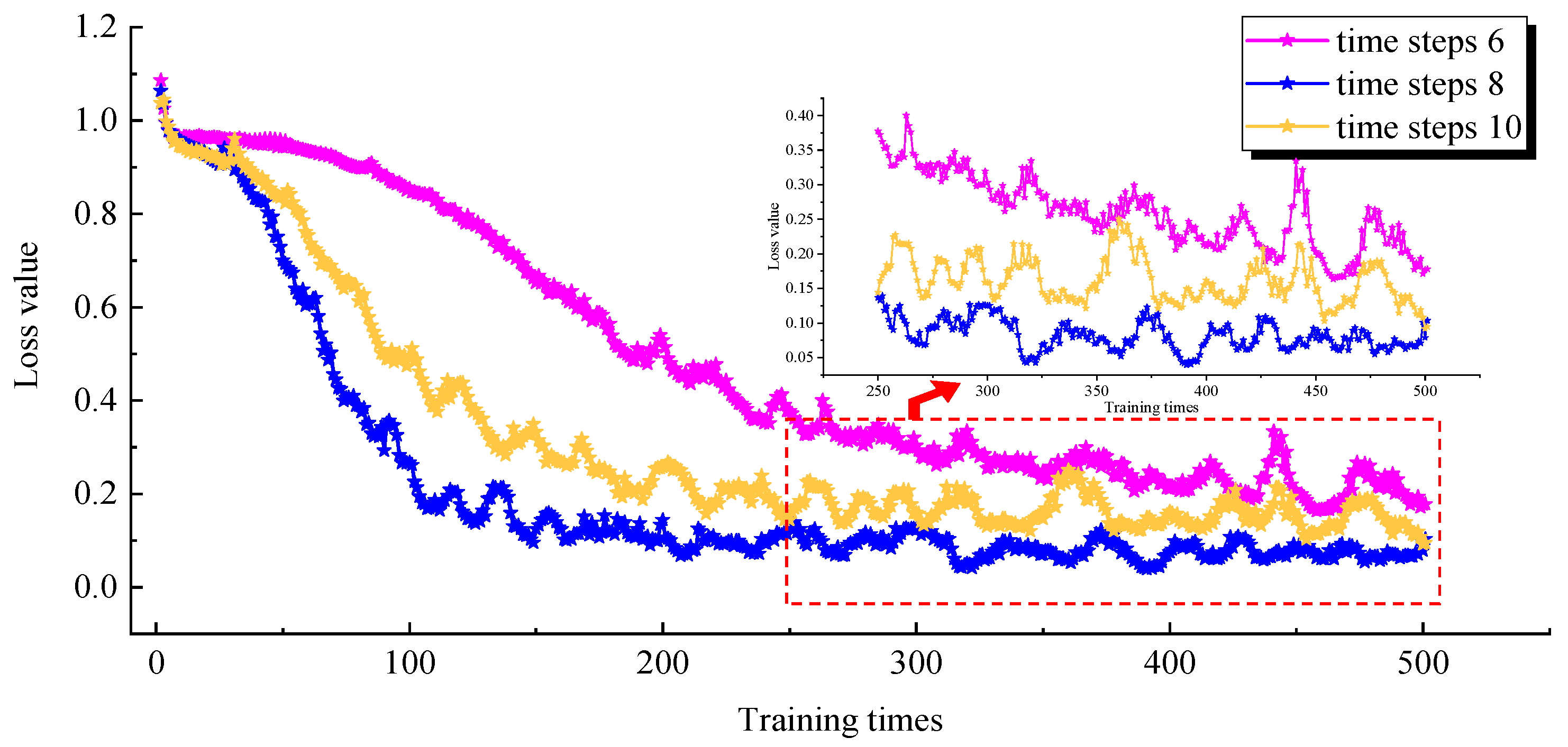
Analytical processing of the data and parameter optimisation of predictive models on the SSF. The GRU neural network requires many parameters to be set when training the data. When predicting gas concentration, the number of neurons, hidden layers, batch sizes and time steps have a large impact on the model and have an influence on the fit and prediction accuracy of the neural network. In this study, these hyperparameters are optimised using the PSO algorithm to optimise the structure of the neural network based on the input data and reduce the training time of the neural network. The features of the number of neurons, hidden layers, batch sizes and time steps are used as features of the particle search for optimisation and are iterated in the PSO algorithm until the optimal solution is output. The steps to achieve the optimisation parameters are as follows:

Step 1: Given some hyperparameters of the GRU neural network, such as network nodes, the number of neurons, hidden layers, batch size and time step of the GRU neural network are initialised and input into the PSO model.

Step 2: Initialise the population size of the particle population, the maximum and minimum values of the particle velocity, the learning rate, the maximum number of iterations and the initial position of the particles.

Step 3: Optimisation training by the PSO model is used to find the best position; obtain and record the optimal solution and update the best position of the particle.

Step 4: After the PSO algorithm training, stop iteration and output the best parameter value when the parameter meets the set condition; otherwise, return to step 3 and continue training.

Step 5: The hyperparameters optimised by the PSO algorithm are fed into the GRU network model as the initial hyperparameters of the GRU neural network to be trained, and then, the predicted values are output. Finally, the fitted curve of the predicted and test data can be derived.

3. Experimental Section

3.1. Experimental Environment and Data Sources

To verify the usefulness of the SSF in this paper, a Spark Streaming experimental cluster was built to verify the example using coal mine methane data. One host was chosen for the experiments, and three virtual machines were deployed on this host with the host master as the master node to control the operation of the whole cluster and the remaining three virtual machines as slave nodes of the master, which were responsible for receiving information. The host configuration is shown in

Table 1. Host configuration.

Projects	Configuration
CPU	Intel (R) Core (TM) i5-8400 (2.80 GHz)
RAM	8 GB
Hard Disk	1 T
Internet speed	100 Mb/s

.

The Python language is used to build models for data pre-processing, model optimisation, model prediction and error analysis, and each part of the process is packaged and imported into the SSF, allowing it to perform data batch processing. The gas concentration at the working face is used as an example for gas prediction and early warning analysis, and a further prediction and early warning analysis is carried out on the model using the gas concentration at the upper corner, inlet gas and return gas concentration data. Two thousand sets of gas concentration data were collected from the working face, and the framework for the data collection and analysis is shown in Figure 4. The first 1800 datasets are used as the training set for model training, and the last 200 sets are used as the test set for prediction and warning analysis according to the time series.

3.2. Optimisation of Predictive Model Parameters

In PSO-GRU, the training set and the test were divided at a ratio of 9:1. The optimisation function is Adam, the activation function is tanh, the learning rate is 0.01 and the training epoch is 500 times. The PSO-GRU model was trained with the minimum loss value as the tuning criterion. The comparison of the number of neurons in the hidden layer, the number of hidden layers, the batch size and the time step are analysed separately to find the best.

(1)

Optimisation of the number of neurons in the hidden layer

The number of neurons in the hidden layer leads to underfitting if there are too few, and too many neurons also leads to poor training results. Thus, in this paper, we set the number of neurons in the range of 32~128. Through extensive experiments, it was found that the training effect is relatively good when the number of neurons is 32, 64 and 128. To further determine the number of neurons, the loss values were compared for 32, 64 and 128 neurons. The process of optimising the number of neurons and the training error is shown in Figure 5 and

Table 2. Comparison of loss values for different numbers of hidden layer neurons.

Number of Neurons in the Hidden Layer	32	64	128
MAE	0.0136	0.0113	0.0164
RMSE	0.0181	0.0139	0.0207
R2	0.904	0.942	0.873

.

As seen in Figure 5 above, the rate of decline of the loss values differs for the three different numbers of hidden layer neurons. The number of neurons is considerably slower for 32 and 128, and the error fluctuates substantially after 400 training sessions. If the number of neurons is 64, the loss value decreases the fastest and converges to 0.1 after 150 training cycles, and the loss value decreases smoothly throughout the training process without major fluctuations. Table 2 shows that the MAE and RMSE for 64 neurons are 0.0113 and 0.0139, respectively, which are smaller than the MAE and RMSE for the other two parameters, proving that the error of the model is smaller and R² is 0.942, which is a good fit. The best model training effect was obtained when the number of neurons was 64 after the comparison of the three results.

(2)

Hidden layer optimisation

For general datasets, 1~2 hidden layers are sufficient, but for complex datasets involving time series and computer vision, additional layers are needed. The dataset studied in this paper has strong time series characteristics, so the range of hidden layers is set to 1~3 for the comparative analysis, comparing the training effects of different hidden layers and comparing the change process of loss values under 1, 2 and 3 hidden layers. The process of optimising the number of hidden layers and the training errors is shown in Figure 6 and

Table 3. Comparison of the loss values for different numbers of hidden layers.

Number of Hidden Layers	1	2	3
MAE	0.0148	0.0113	0.0157
RMSE	0.0189	0.0139	0.0199
R2	0.895	0.942	0.882

.

As seen in Figure 6, when the hidden layer is 1 layer, although there is no large fluctuation in the loss value during the training process, the model loss value converges more slowly. When the hidden layer is 3 layers, the loss value of the model decreases faster, and the loss value decreases to 0.15 at approximately the 250th training session, but the loss value of the model fluctuates more during the training process. When the number of hidden layers is 2, the model converges quickly, the loss value drops to 0.1 at the 150th training session and the loss value of the model decreases smoothly without large fluctuations throughout the training process. Table 3 shows that the MAE, RMSE and R² are the most effective among the three parameters when the number of hidden layers is 2. Therefore, the number of hidden layers is 2.

(3)

Batch size optimisation

The batch size is the number of samples selected for one training, and its size affects the optimisation degree and speed of the model. A size that is too small leads to inefficiency and failure to converge, and a size that is too large leads to CPU overload. It was found that, in the preliminary experimental process when the batch size is greater than 256, the convergence effect is better; therefore, to compare the training effect of different batch sizes, in this paper, the range of batch sizes is set to 256~1024 for the comparative analysis. The batch size optimisation process and training errors are shown in Figure 7 and

Table 4. Comparison of the loss values for different batch sizes.

Batch Size	256	512	1024
MAE	0.0169	0.0113	0.0143
RMSE	0.0224	0.0139	0.0189
R2	0.865	0.942	0.894

.

As seen in Figure 7 above, the trends of the loss value curves for the three different batch sizes are obviously different. When the batch size is 256, the loss value decreases slowly, the loss value fluctuates severely throughout the training process and, finally, the loss value converges to 0.2. When the batch size is 1024, the loss value decreases quickly, fluctuates more smoothly and, finally, converges to 0.2 at the 350th time. When the batch size is 512, the loss value decreases quickly, the training process is more stable and the training effect is the best. The MAE and RMSE of the model were the smallest, and R² was the largest for batch size 512 in Table 4, which was the best overall performance.

(4)

Time step optimisation

The time step is the difference between the two time points before and after. The size of the time step generally depends on the system properties and the purpose of the model. To compare the prediction effects of different time steps, the range of time steps is set to 6~10 for the comparative analysis. The time step optimisation process and training errors are shown in Figure 8 and

Table 5. Comparison of errors using different step sizes.

Time Step	6	8	10
MAE	0.0165	0.0113	0.0153
RMSE	0.0226	0.0139	0.0204
R2	0.856	0.942	0.874

.

As seen in Figure 8, when the time step is 6, the loss value decreases slowly and fluctuates considerably as the loss value tends to stabilise. When the step size is 10, the training becomes faster, but the loss values fluctuate severely throughout the training process. The best training result was achieved when the step size was 8, with the loss value falling fast and fluctuating smoothly and finally converging to 0.2 at the 350th time. Additionally, combined with the fact that the MAE and RMSE of the model were the smallest and R² was the largest at the time step size of 8 in Table 5, it was determined that the time step size was 8.

According to the above study, the optimal parameters of PSO-GRU are obtained. The number of neurons in the hidden layer is 64, the hidden layer is 2, the batch size is 512 and the time step is 8. According to the specific optimised parameters determined above, the training and prediction of the gas concentration data of the working face are carried out, and Figure 9 is obtained. The prediction results based on the PSO-GRU model have a better fit with the real values, the iteration speed during the training process is faster and the prediction accuracy is considerably improved, which shows that the model has strong applicability in the process of gas concentration prediction.

3.3. Early Warning Analysis for Gas Concentration Prediction

Prior to the early warning of gas concentration at the working face, the gas threshold is determined based on the gas concentration collected by the gas sensor and the gas prediction value x_i derived from the prediction model, and then, the warning interval is determined based on the measured data. The mean μ_x and variance σ_x are calculated from the measured gas concentration data and the duration of the increase in gas concentration t_h. The confidence interval and the duration of the increase in gas concentration are used as the warning judgement, and the following classification of the warning level is made.

(1)

Warning level I

When the predicted value of gas concentration is below the warning threshold and the predicted value falls within the 85% confidence interval, x_i < w_s and x_i ∈ [μ − 1.44σ, μ + 1.44σ], the situation is considered normal and no warning is given. When the predicted value of gas concentration falls within the upper limit of the 85–95% confidence interval and the gas concentration continues to increase within 15 min, x_i ∈ [μ + 1.44σ, μ + 1.96σ], t_h > 15 min is set as warning level I, the trend of gas concentration change needs to be followed in time and the cause of the gas concentration increase needs to be identified.

(2)

Warning Level II

When the gas prediction is lower than the warning threshold but falls within the upper limit of the warning threshold and 95% confidence interval, μ + 1.96σ < x_i < w_s, and the gas concentration prediction continues to increase within 30 min, t_h > 30 min. It is designated warning level II, and the cause needs to be identified in time, and appropriate measures need to be taken to proceed.

According to the principle of gas concentration warning, an analysis of anomalous values and determination of warning thresholds, the design of gas concentration warning can be carried out. First, a gas concentration prediction model is established based on the characteristics of the gas data, and gas concentration prediction values are obtained for the working face. Finally, the gas concentration of the working face warning thresholds is determined based on the basic indicators and threshold division of the working face gas concentration warning, and then, the gas warning levels are divided.

The mean is μ_x = 0.6467 and variance σ_x = 0.0572 for the gas concentration-related indicators at the working face. The results of the gas prediction using the PSO-GRU model are shown in Figure 9. According to the gas threshold determination method proposed above, it is known that the 95% confidence interval range is [0.5342, 0.7593], and the 85% confidence interval range is [0.5639, 0.7284]. Therefore, the gas warning level I range is [0.7284, 0.7593], and the gas concentration data continuously increase within 15 min. The gas warning level II is [0.7593, 1], and the gas concentration data continue to increase within 30 min. To better visualise the effect of the warning, the warning levels are quantified by using 0 for normal, 1 for warning level I and 2 for warning level II, and the gas concentration warning results are shown in Figure 10.

As seen in the gas prediction graph, the PSO-GRU model has a good prediction, with a model fit of 0.974, which can be used for early warning of gas concentrations. As shown in Figure 10, the gas concentration remains normal without major fluctuations until the 35th sample point. From the 35th sample n point to the 60th sample point, the predicted gas concentration continues to be high, with warning level I and warning level II occurring. From the 60th to the 170th sample point, the gas concentration decreases and then rises again at the last 20 sample points to warning level II. Based on the comparison between the measured and predicted values, the warning situation is generally consistent with the actual situation.

4. Result and Discussion

To verify the usefulness and efficiency of the SSF, the upper corner gas data, return airflow gas data and inlet airflow gas data were imported into the SSF for verification. Error comparisons were carried out using three evaluation metrics (MAE, RMSE and R²) for the upper corner, return airflow and inlet airflow gas data. The early warning model was analysed using prediction accuracy. Early warning levels were calculated for the gas concentrations in the upper corner, inlet airflow and return airflow according to the determination method of the gas warning rules in Section 3.3, and the warning ranges were obtained as shown in

Table 6. Warning range for gas concentrations.

Gas Concentration Zones	Early Warning Level I	Early Warning Level II
Upper corner	[0.752, 0.776]	[0.776, 1]
Inlet airflow	[0.396, 0.435]	[0.435, 1]
return airflow	[0.712, 0.736]	[0.736, 1]

. The upper corner, inlet airflow and return airflow gas concentration prediction and warning diagrams are shown in Figure 11, Figure 12, Figure 13, Figure 14, Figure 15 and Figure 16.

According to the prediction and warning figures, it can be seen that the warning effect is basically in line with the actual situation. To further verify the prediction effect of the prediction model, the MAE, RMSE and R² were calculated for the gas concentration at the working face, the gas concentration at the upper corner, the gas concentration in the return airflow and the gas concentration in the inlet airfield, respectively. The errors for the four different gas distribution areas are shown in

Table 7. MAE, RMSE and R² of the gas concentration prediction results for different areas.

Gas Distribution Areas	MAE	RMSE	R2
Gas concentration at the working face	0.0121	0.0159	0.974
Upper corner gas concentration	0.0134	0.0168	0.965
Return airflow gas concentration	0.0130	0.0162	0.968
Gas concentration in the inlet air stream	0.0141	0.0171	0.962

, and it can be seen from the prediction errors that the model’s overall prediction error is low. The prediction accuracy of the gas concentration at the working face, upper corner and return airflow are shown in

Table 8. Prediction accuracy in different areas.

Gas Distribution Areas	Predicted Sample Size	Number of Accurate Predictions	Accuracy Rate/%
Gas concentration at the working face	200	180	90
Upper corner gas concentration	200	183	91.5
Return airflow gas concentration	200	189	94.5
Gas concentration in the inlet air stream	200	191	95.5

and Figure 17. The model achieved prediction accuracies of 90%, 91.5%, 94.5% and 95.5% with high overall prediction rates. The working face is a complex environment, with many factors affecting the gas concentration; therefore, the prediction accuracy of the working face is relatively low. In contrast, the inlet tunnel has relatively few factors affecting the gas concentration; therefore, the prediction accuracy is the highest.

It can be seen from the prediction accuracy in different areas that the overall prediction accuracy of the model is high, all of which can exceed 90%.

Table 9. Accuracy of the gas concentration warnings at two warning levels.

Early Warning Level	Early Warning Sample Size	Number of Accurate Warning	Accuracy Rate/%	False Alarm Rate/%
Warning level I	59	56	94.9	4.1
Warning level II	36	35	97.2	2.8
Total	95	91	95.7	4.3

shows that the warning accuracy for the two warning levels is 94.9% and 97.2%, respectively, which is a high warning accuracy rate. To further validate the advantages of the high running efficiency of the model proposed in this paper, a control variable approach was used to compare the running time of the model using the SSF (see Figure 18) and the model without the SSF (see Figure 19). Additionally, it can be seen that the overall running time of the model is shortened after the SSF is used. When using the same method to compare the run times with and without the virtual machine, it was found that the average warning time was longer when the model was run locally without the virtual machine, with a slow increase in warning speed when one virtual machine was turned on and faster when three virtual machines were turned on. It can be seen that the alert time based on the SSF is fast, which greatly improves the efficiency of the alert and effectively validates the SSF’s ability to process large volumes of data quickly and efficiently. Combining SSF with gas concentration monitoring enables accurate predictions and graded warnings of gas concentrations and support for mine management in decision making in the event of a sudden increase in gas concentration. This provides a guarantee for the safe production of coal mines.

5. Conclusions

With the development of intelligent coal mines, the highly efficient real-time online analysis of a gas concentration has become an important technical tool for intelligent gas monitoring, providing an important guarantee for the safe and stable daily operations of coal mines. In this study, we propose an overlay model for gas concentration prediction and early warning that combines the PSO model and the GRU model under the SSF, which can achieve high efficiency and high accuracy of gas concentration predictions and early warning analyses.

(1)

The SSF, particle swarm optimisation algorithm and gated recurrent neural network are introduced and fused. Moreover, we also propose a new gas prediction and warning model, the SSPG model.

(2)

With the optimisation of the model parameters and further prediction and early warning analysis of gas concentration, the experimental results show that the model can better predict and warn the gas concentration early when the prediction error is small, and the early warning accuracy can reach more than 90%.

(3)

The application performance of the model is verified. A comparative analysis of the operational efficiency of the model was carried out using the control variables method. The results show that the model is able to complete the prediction and early warning of gas concentration with high efficiency and accuracy, fast data processing speed and high fault tolerance. This study is of great importance to the development of intelligent gas monitoring in coal mines. Next, we will investigate the correlation between the gas field and the wind flow field. The airflow regulation scheme can be quickly proposed in the event of a sudden increase in gas concentration, decision support for daily gas concentration management in coal mines.

References

1. Zhao, H.B.; Li, J.Y.; Liu, Y.H.; Wang, Y.K.; Wang, T.; Cheng, H. Experimental and measured research on three-dimensional deformation law of gas drainage borehole in coal seam. Int. J. Min. Sci. Technol. 2020, 30, 397–403. [Google Scholar] [CrossRef]
2. Li, Z.H.; Wang, E.Y.; Ou, J.C.; Liu, Z.T. Hazard evaluation of coal and gas outbursts in a coal-mine roadway based on logistic regression model. Int. J. Rock Mech. Min. Sci. 2015, 80, 185–195. [Google Scholar] [CrossRef]
3. Huang, Y.X.; Fan, J.D.; Yan, Z.G.; Li, S.G.; Wang, Y.P. A Gas Concentration Prediction Method Driven by a Spark Streaming Framework. Energies 2022, 15, 5335. [Google Scholar] [CrossRef]
4. Cheng, L.; Li, L.; Li, S.; Ran, S.L.; Zhang, Z.; Zhang, Y. Prediction of gas concentration evolution with evolutionary attention-based temporal graph convolutional network. Expert Syst. Appl. 2022, 200, 116944. [Google Scholar] [CrossRef]
5. Li, Q.G.; Lin, B.Q.; Zhai, C. A new technique for preventing and controlling coal and gas outburst hazard with pulse hydraulic fracturing: A case study in Yuwu coal mine, China. Nat. Hazards 2015, 75, 2931–2946. [Google Scholar] [CrossRef]
6. Huang, Y.X.; Fan, J.D.; Yan, Z.G.; Li, S.G.; Wang, Y.P. Research on Early Warning for Gas Risks at a Working Face Based on Association Rule Mining. Energies 2021, 14, 6889. [Google Scholar] [CrossRef]
7. Fu, G.; Zhao, Z.Q.; Hao, C.B.; Wu, Q. The Accident Path of Coal Mine Gas Explosion Based on 24Model: A Case Study of the Ruizhiyuan Gas Explosion Accident. Processes 2019, 7, 73. [Google Scholar] [CrossRef] [Green Version]
8. Wang, C.; Wei, L.K.; Hu, H.Y.; Wang, J.R.; Jiang, M.F. Early Warning Method for Coal and Gas Outburst Prediction Based on Indexes of Deep Learning Model and Statistical Model. Front. Earth Sci. 2022, 10, 811978. [Google Scholar] [CrossRef]
9. Zhao, Y.; Niu, X.A. Experimental Study on Work of Adsorption Gas Expansion after Coal and Gas Outburst Excitation. Front. Earth Sci. 2022, 10, 120. [Google Scholar] [CrossRef]
10. Tutak, M.; Brodny, J. Predicting Methane Concentration in Longwall Regions Using Artificial Neural Networks. Int. J. Environ. Res. Public Health 2019, 16, 1406. [Google Scholar] [CrossRef]
11. Zeng, J.; Li, Q.S. Research on Prediction Accuracy of Coal Mine Gas Emission Based on Grey Prediction Model. Processes 2021, 9, 1147. [Google Scholar] [CrossRef]
12. Xu, Y.H.; Meng, R.T.; Zhao, X. Research on a Gas Concentration Prediction Algorithm Based on Stacking. Sensors 2021, 21, 1597. [Google Scholar] [CrossRef] [PubMed]
13. Liu, C.; Li, S.G.; Yang, S.G. Gas emission quantity prediction and drainage technology of steeply inclined and extremely thick coal seams. Int. J. Min. Sci. Technol. 2018, 28, 415–422. [Google Scholar]
14. Cong, Y.; Zhao, X.M.; Tang, K.; Wang, G.; Hu, Y.F.; Jiao, Y.K. FA-LSTM: A Novel Toxic Gas Concentration Prediction Model in Pollutant Environment. IEEE Access 2022, 10, 1591–1602. [Google Scholar] [CrossRef]
15. Zhang, T.; Song, S.; Li, S.; Ma, L.; Pan, S.; Han, L. Research on Gas Concentration Prediction Models Based on LSTM Multidimensional Time Series. Energies 2019, 12, 161. [Google Scholar] [CrossRef] [Green Version]
16. Lyu, P.; Chen, N.; Mao, S.; Li, M. LSTM based encoder-decoder for short-term predictions of gas concentration using multi-sensor fusion. Process Saf. Environ. Prot. 2020, 137, 93–105. [Google Scholar] [CrossRef]
17. Jia, P.T.; Liu, H.D.; Wang, S.J.; Wang, P. Research on a Mine Gas Concentration Forecasting Model Based on a GRU Network. IEEE Access 2020, 8, 38023–38031. [Google Scholar] [CrossRef]
18. Xu, N.K.; Wang, X.Q.; Meng, X.R.; Chang, H.Q. Gas Concentration Prediction Based on IWOA-LSTM-CEEMDAN Residual Correction Model. Sensors 2022, 22, 4412. [Google Scholar] [CrossRef]
19. Zhang, Y.W.; Guo, H.S.; Lu, Z.H.; Zhan, L.; Hung, P.C.K. Distributed gas concentration prediction with intelligent edge devices in coal mine. Eng. Appl. Artif. Intell. 2020, 92, 103643. [Google Scholar] [CrossRef]
20. Dey, P.; Saurabh, K.; Kumar, C.; Pandit, D.; Chaulya, S.K.; Ray, S.K.; Prasad, G.M.; Mandal, S.K. t-SNE and variational auto-encoder with a bi-LSTM neural network-based model for prediction of gas concentration in a sealed-off area of underground coal mines. Soft Comput. 2021, 25, 14183–14207. [Google Scholar] [CrossRef]
21. Diaz, J.; Agioutantis, Z.; Hristopulos, D.T.; Schafrik, S.; Luxbacher, K. Time Series Modeling of Methane Gas in Underground Mines. Ming Metall. Explor. 2022, 39, 1961–1982. [Google Scholar] [CrossRef]
22. Matteussi, K.J.; Dos Anjos, J.C.S.; Leithardt, V.R.Q.; Geyer, C.F.R. Performance Evaluation Analysis of Spark Streaming Backpressure for Data-Intensive Pipelines. Sensors 2022, 22, 4756. [Google Scholar] [CrossRef] [PubMed]
23. Cheng, D.Z.; Zhou, X.B.; Wang, Y.; Jiang, C.J. Adaptive Scheduling Parallel Jobs with Dynamic Batching in Spark Streaming. IEEE Trans. Parallel Distrib. Syst. 2018, 29, 2672–2685. [Google Scholar] [CrossRef]
24. Liu, L.T.; Wen, J.B.; Zheng, Z.X.; Su, H.S. An improved approach for mining association rules in parallel using Spark Streaming. Int. J. Circuit Theory Appl. 2021, 49, 1028–1039. [Google Scholar] [CrossRef]
25. Ren, M.L.; Huang, X.D.; Zhu, X.X.; Shao, L.J. Optimized PSO algorithm based on the simplicial algorithm of fixed point theory. Appl. Intell. 2020, 50, 2009–2024. [Google Scholar] [CrossRef]
26. Nobile, M.S.; Cazzaniga, P.; Besozzi, D.; Colombo, R.; Mauri, G.; Pasi, G. Fuzzy Self-Tuning PSO: A settings-free algorithm for global optimization. Swarm Evol. Comput. 2018, 39, 70–85. [Google Scholar] [CrossRef]
27. Jain, M.; Saihjpal, V.; Singh, N.; Singh, S.B. An Overview of Variants and Advancements of PSO Algorithm. Appl. Sci. 2022, 12, 8392. [Google Scholar] [CrossRef]
28. Wu, L.Z.; Kong, C.; Hao, X.H.; Chen, W. A Short-Term Load Forecasting Method Based on GRU-CNN Hybrid Neural Network Model. Math. Probl. Eng. 2020, 2020, 1428104. [Google Scholar] [CrossRef] [Green Version]
29. Zhang, Y.G.; Tang, J.; Cheng, Y.M.; Huang, L.; Guo, F.; Yin, X.J.; Li, N. Prediction of landslide displacement with dynamic features using intelligent approaches. Int. J. Min. Sci. Technol. 2022, 32, 539–549. [Google Scholar] [CrossRef]
30. Mahjoub, S.; Chrifi-Alaoui, L.; Marhic, B.; Delahoche, L. Predicting Energy Consumption Using LSTM, Multi-Layer GRU and Drop-GRU Neural Networks. Sensors 2022, 22, 4062. [Google Scholar] [CrossRef]
Figure 1. Spark Streaming operational architecture diagram.
Processes 11 00220 g001
Figure 2. Input and output structure of the GRU.
Processes 11 00220 g002
Figure 3. Internal structure of the GRU model.
Processes 11 00220 g003
Figure 4. Data acquisition process and analysis.
Processes 11 00220 g004
Figure 5. Optimisation of the number of neurons.
Processes 11 00220 g005
Figure 6. Optimisation of the number of hidden layers.
Processes 11 00220 g006
Figure 7. Batch size optimisation.
Processes 11 00220 g007
Figure 8. Time step optimisation.
Processes 11 00220 g008
Figure 9. PSO-GRU model prediction diagram.
Processes 11 00220 g009
Figure 10. Scatter diagram for predicting gas concentration at the working face.
Processes 11 00220 g010
Figure 11. Predicted gas concentration in the upper corner.
Processes 11 00220 g011
Figure 12. Predicted gas concentration in the return airflow.
Processes 11 00220 g012
Figure 13. Predicted gas concentration in the inlet airflow.
Processes 11 00220 g013
Figure 14. Gas concentration warning in the upper corner.
Processes 11 00220 g014
Figure 15. Gas concentration warning in the return airflow.
Processes 11 00220 g015
Figure 16. Gas concentration warning in the inlet airflow.
Processes 11 00220 g016
Figure 17. Number of accurate predictions and accuracy rate.
Processes 11 00220 g017
Figure 18. Early warning time for the gas concentration in different regions using the SSF.
Processes 11 00220 g018
Figure 19. Early warning times for the gas concentration in different regions without the SSF.
Processes 11 00220 g019