Graphical Tools for Increasing the Effectiveness of Gage Repeatability and Reproducibility Analysis

Abstract

The article deals with the quality of measured data, which is necessary for effective quality management and successful implementation of the concept Industry 4.0 and the related concept Quality 4.0. The quality of the measured data is determined by the properties of the used measurement system, which are evaluated by measurement system analysis (MSA). Attention is paid to increasing the effectiveness of the repeatability and reproducibility analysis often used in practice. The importance of graphical tools of analysis, which are often neglected in practice, is emphasized in this regard, and new or modified graphical tools are proposed. The proposed graphical tools allow more detailed analysis of the data collected for the study and reveal the causes of the measurement system variability. The information obtained by applying these graphical tools is a valuable basis for proposals of appropriate actions to improve the measurement system. The use of the proposed graphical tools is presented in a real study of the repeatability and reproducibility of the measurement system.

1. Introduction

In connection with the application of the concept Industry 4.0 and the related concept Quality 4.0, the requirements for the quality of measured data are significantly increasing. The measured data are a fundamental basis for important decisions, e.g., within the framework of product quality inspection, production process control, monitoring the status of production equipment, diagnostics of products used, evaluation of corrective action effectiveness, implementation of quality improvement activities, etc. The proposed and already used measurement systems require sufficient attention, as an unsatisfactory measurement system can provide misleading information that can lead to poor decisions. Verification of the acceptability of the measurement system is therefore an important part of quality planning and quality improvement and in the automotive industry, it is strictly required [1].

The acceptability of a measurement system is evaluated on the basis of various properties. In the case where the measurement system properties are not suitable, the measured values of the observed quality characteristics do not correspond to reality, and the well-intended interventions into the production process result in wrong decisions that can cause financial losses. Due to this reason, the recognition of the measurement system properties is the basic condition for correct decision making.

The measurement system properties can be evaluated by means of measurement system analyses. Automotive industry suppliers most often use and apply the MSA methodology—Measurement System Analysis [2]. This methodology was created by a trio of American car manufacturers: Chrysler Group LLC, Ford Motor Company and General Motors Corporation.

The article focuses on improving the methodological approach to the analysis of the repeatability and reproducibility of the measurement system, where insufficient attention is paid to the graphical tools of the analysis. Modified as well as completely new graphical tools of analysis are suggested, which will better reveal the effect of the various factors involved in the variability of the measurement system.

2. Properties of the Measurement System

The main properties of a measurement system that determine the quality the measured data include the following [2]:

• sensitivity;
• drift (stability);
• consistency;
• accuracy;
• bias;
• linearity;
• uniformity;
• precision;
• repeatability;
• reproducibility
• uncertainty.

These properties can be divided into location characteristics and variability characteristics. The characteristics of location include drift (stability), accuracy, bias and linearity, and the characteristics of variability concern sensitivity, consistency, precision, repeatability, reproducibility and uniformity. Uncertainty, which characterizes an estimated range of values in which the true value is believed to be contained [2] takes into consideration both variability and location.

The sensitivity is defined as the smallest input signal that results in a detectable (discernible) output signal for a measurement device. An instrument should be at least as sensitive as its unit of discrimination [2].

The drift or the stability is defined as the change in bias over time, and the consistency is defined as a degree of change of repeatability over time. Assessment of these properties is realized using control charts constructed for chosen measures of location and variability. A stable and consistent measurement process is in statistical control. An evaluation of the drift (stability) and consistency of a measurement system should be performed first. Only when it is confirmed that the properties of the measurement system do not change over time (the measurement system is stable and consistent) does it make sense to carry out further analyses of the measurement system.

The accuracy characterizes the closeness of agreement between an observed value and the accepted reference value, and the bias is defined as the difference between the average of repeated measurements and the reference value [2]. The bias represents a level of systematic error of the measurement system. It can be positive or negative; the optimal value of bias is zero.

A change in the bias over the normal operating range is defined as linearity. It is evaluated by regressing the deviations of the measured values from the reference values of the measured samples on the reference value. Linearity is considered acceptable if the regression parameter estimates are not statistically significant [2]. The measurement system variability is a combination of the measurement system repeatability and reproducibility. The measurement system repeatability is closely related to the term of measurement precision, which is expressed as “closeness” of repeated measurements to each other and describes the expected variation of repeated measurements [2]. The repeatability itself represents a measurement precision under repeatability conditions. The repeatability conditions are when independent measurement results are obtained by the one operator by the same method, with the same measuring device, at the same measurement site and within the shortest time period.

The reproducibility of a measurement system represents the variability of the mean values of repeated measurements of the same characteristic taken under different conditions. This is most often the case when the measurements are taken by different operators, but it can also be a situation where one operator takes measurements with different gauges or in different environments.

The uniformity is defined as a change in repeatability over the normal operating range. The uniformity analysis complements the linearity analysis of a measurement system; it evaluates whether the repeatability of the measurement system depends on the magnitude of the measured value. In practice, uniformity analysis is often neglected.

In the automotive industry, the MSA methodology [2] and the VDA 5 methodology [3] are most often used to evaluate the properties of the measurement system. Another possibility is to evaluate the capability of the measurement systems using the C_g and C_gk indices, which evaluate the repeatability and bias of the measurement system [4,5].

In practice, much attention is paid to properties related to the variability of the measurement system. This is because these properties are, along with bias, the basis for estimating the measurement uncertainty. In the field of quality management, for example, this has a direct impact on product conformity assessment. Conformity of a product can be clearly confirmed only if the entire measurement uncertainty interval lies within a tolerance. If only part of the uncertainty interval lies within the tolerance, the result of the conformity test is inconclusive [6]. The role of measurement uncertainty in conformity assessment is described in further detail in the document of the Joint Committee for Guides in Metrology JCGM 106:2012 [7].

Information about the properties of a measurement system is also important when evaluating the capability of the production process. Not only the variability of the production process but also the variability of the measurement system contributes to the variability of the monitored quality characteristics of the manufactured products. If the contribution of the variability of the measurement system is significant, it can also lead to the conclusion that a capable production process can be evaluated as incapable [8].

3. Gauge Repeatability and Reproducibility Analysis

The evaluation of repeatability and reproducibility of the measurement system (Gage R&R analysis) is implemented because it is mostly impossible to ensure constant conditions (repeatability conditions) during the measurement process in practice. The actual measurement conditions usually vary, whereas the operator taking the measurements is the element that is most frequently changed. The study on repeatability and reproducibility of the measurement system can be done using several different procedures. The MSA methodology [2] describes three methods of analysis:

• Range Method;
• Average and Range Method;
• ANOVA (Analysis of Variance).

The Range Method is also called the “short method” and enables a quick approximation of the measurement variability. It provides the whole picture of the measurement system because it does not decompose the variability into the repeatability and reproducibility. This distinction is made possible by the other two mentioned methods; the ANOVA method is also able to indicate variability caused by interactions between operators and samples.

3.1. Average and Range Method

This method is often used in practice. This is mainly related to the fact that the individual steps of the analysis use simple calculations, and the entire evaluation can be performed without the use of a computer or with the use of a relatively simple spreadsheet-based application.

During the preparative phase, it is necessary to define all basic parameters of the analysis, i.e., the number of operators, number of measured samples and the number of repeated measurements per each sample. There should be at least ten measured samples [2], and this minimum number is most often used in examples and in practice. In a note to this requirement, the MSA manual [2] recommends that the number of samples be greater than 15 to ensure sufficient confidence in the results.

Each sample should be measured by each operator two times at least, and the number of operators should be based on the real usage of the measurement system. The choice of the measured samples is very important. The samples should cover the whole production range of the monitored characteristic for the purpose of the standard analysis procedure.

The measurement phase involves an assurance of measurement independence. Independence can be achieved by taking measurements in random order. The operators do not know which sample they are measuring or the results of previous measurements. Due to these reasons, the monitoring of measurement and data recording is performed by the employee in charge. Before the actual evaluation, it is necessary to verify the independence of the data and the normality of the data with appropriate tests.

The analysis evaluation is divided into several coherent steps as described in the MSA manual [2]. By following the prescribed procedures, which include both numeric and graphical evaluation, the repeatability (equipment variation (EV)) and reproducibility (appraiser variation (AV)) are evaluated. On the basis of their values, it is possible to calculate repeatability and reproducibility of the measurement system (GRR) according to the following Relation [2]:

$$\mathrm{GRR}=\sqrt{{\left(\mathrm{EV}\right)}^2+ {\left(\mathrm{AV}\right)}^2}$$

(1)

As criteria of the measurement system acceptability, the percentage share of the GRR in total variation and number of distinct categories (ndc) are used. They are calculated using Formulas (2) and (3) [2].

$$\%\mathrm{GRR}=\frac{\mathrm{GRR}}{\mathrm{TV}}\cdot 100$$

(2)

$$\mathrm{ndc}=1.41\cdot \frac{\mathrm{PV}}{\mathrm{GRR}}$$

(3)

$$\mathrm{TV}=\sqrt{{\left(\mathrm{GRR}\right)}^2+{\left(\mathrm{PV}\right)}^2}$$

(4)

where TV denotes total variation, and PV is part variation.

The conclusion regarding the acceptability of the measurement system should be made after evaluating both the indicators. Three situations may occur, as described in

Table 1. Gage R&R analysis acceptance criteria [2].

Criteria Values	Acceptability of Measurement System
%GRR ≤ 10% and ndc ≥ 5	The measurement system is acceptable.
10% < %GRR ≤ 30% and ndc ≥ 5	The measurement system may be acceptable for some applications, and should be approved by the customer. The decision should by based upon, for example, importance of application measurement, cost of measurement device, or cost of rework or repair.
%GRR > 30% or ndc < 5	The measurement system is unacceptable, and it must be improved.

[2].

It should be noted that the measurement system acceptability criteria (%GRR, ndc) are interdependent [9]. An increase in the value of %GRR will be reflected in the decrease of ndc.

3.2. ANOVA

In the case of using the ANOVA method, the total variability can be divided into repeatability–equipment variation (EV), reproducibility–appraiser variation (AV), part variation (PV) and the variability caused by the interactions between operators and parts (INT). The evaluation of the Gage R&R analysis using this method allows a more objective evaluation of the variability of the measurement system, as it also provides additional information on how much of the total variability is caused by the interactions among the individual operators and parts [2]. If these interactions are statistically significant, their value is expressed separately, and the repeatability and reproducibility are calculated as follows:

$$\mathrm{GRR}=\sqrt{{\left(\mathrm{EV}\right)}^2+{\left(\mathrm{AV}\right)}^2+ {\left(\mathrm{INT}\right)}^2}$$

(5)

Before Gage R&R analysis using the ANOVA method, it is necessary to test the independence of the data, the normality of the data and the homogeneity of variance.

4. Proposal of Graphical Tools for Effective Gage R&R Analysis

The repeatability and reproducibility of a measurement system should not be evaluated only by numerical methods. Appropriate graphical tools should also be an important part of the analysis. Their use provides valuable information not evident from the numerical results and greatly facilitates identification of causes of non-conforming properties of the measurement system.

Publications describing the methodology of Gage R&R analysis usually do not pay significant attention to graphical tools of analysis. Mostly, they use range control charts and average control charts, where the values are plotted in random order according to the sample numbers. In [10], only a range control chart is presented in the methodology of analysis, and in [11], a range control chart and average control chart are presented. Somewhat extended options for using graphical tools are presented in [12], where, in addition to range and average control charts, a main effect chart for operators and mean range chart for operators are used. In the main effect chart for operators, the averages of all measurements of individual operators are plotted, and modified control limits are added, which make it possible to evaluate whether averages between operators do not show significant differences. The mean range chart for operators is based on a similar principle; it evaluates whether there are significant differences between the average variation ranges of repeated measurements for individual operators.

Based on the literature review of published articles dealing with repeatability and reproducibility analysis, it can be concluded that these articles do not adequately address the possibilities of developing graphical tools of analysis. An example of a work that deals more closely with the use of graphical tools in the analysis of repeatability and reproducibility is [13], where the author focuses on their use in identifying systematic and random interactions between operators and samples.

In the published case studies, the standard graphical outputs of the used software are presented, but in many cases the graphical tools of analysis are not presented at all. If graphical tools of analysis are used, they are usually the standard graphical outputs of the Minitab software, which uses most of the diagrams described in the MSA manual [2] (range or standard deviation control chart, average control chart, diagram of individual values, box and whisker plot and interaction plot). These graphical outputs provide valuable additional information to the numerical results of the analysis, but they do not allow for a more detailed analysis of all possible causes of the variability of the measurement system. The disadvantage is also that in the graphical outputs, the data are displayed according to the sample numbers, i.e., in a random order, which limits their informativeness.

An example of a work using the graphical outputs of Minitab software is [14], in which the authors evaluated and compared the variability of measurements between a manual instrument of measurement and a laser instrument during aircraft production processes. Another example of the use of these standard graphical outputs is [15], where Gage R&R analysis was used to compare two methods of measurement performed on a coordinate measurement machine. Numerical and graphical outputs confirmed that measurement in automatic (programmable) mode produces better results than measurement in manual mode. In addition, in [16], where the authors used Gage R&R analysis to estimate the uncertainties of measuring the gap and flush in a car assembly line by hand-held non-contact laser scanners, these standard graphical tools were used.

In some published case studies, graphical tools of analysis are not presented at all. While these tools may have still have been used in these studies, the authors did not consider them to be an important part of the Gage R&R analysis results. An example of such a case study is [17], where the authors used various methods of estimating the variance components in a measurement system and conducted a comparison of the method of ranges with that of ANOVA. They developed Excel templates to perform calculations, but no graphical outputs were presented. The graphical outputs of the Gage R&R analysis are also not presented in [18], where the authors proposed a method for the measured values that can be characterized by a simple linear profile, which was then applied to the spring length and elasticity measurement.

In the next chapters, appropriate graphical tools, which should be an integral part of the effective analysis of the repeatability and reproducibility of a measurement system, are proposed. Some were created as a suitable modification of the graphical tools mentioned in the MSA manual [2], while some are newly proposed.

4.1. The Essence of the Proposed Graphical Tools

Product samples are randomly numbered when collecting data for the Gage R&R analysis, and this random order is also used when applying graphical tools of analysis. Some authors of this article previously recommended [19] that samples should no longer be arranged randomly when evaluating data in graphs and that they should be arranged by size. This arrangement has no effect on the numerical results of the analysis, but it significantly improves the clarity and explanatory power of the graphs. This is evident, for example, from the comparison of Figure 1 and Figure 2, where box and whisker plots are used to assess the symmetry of the distribution of all the measurements of the individual product samples and to identify any outliers.

In this article, the authors propose that for those graphical tools where it makes sense, the value of the measured characteristic of a given sample, represented by the average of all its measurements, is directly plotted in graphs. An alternative could be to use reference values for individual product samples if they are available. The added value of this solution is mainly an increase in objectivity in evaluating the dependence of some of the properties of the measurement system on the magnitude of the measured characteristic and clearer information on how the measured product samples cover the production range.

The authors recommend that all graphical tools be applied at the beginning of the Gage R&R analysis before the numerical evaluation. The reason is that, with the help of these graphical tools, it is possible to identify some weaknesses in the measurement system and reveal their causes. Once these causes have been eliminated, the affected measurements can be repeated.

4.2. Suitable Graphical Tools of Gage R&R Analysis

The proposed graphical tools were applied to the real data shown in

Table 2. Measured data of nut height (in mm) [20].

Operator	Trials	Sample Number
		1	2	3	4	5	6	7	8	9	10
A	1	10.96	10.90	10.67	10.35	10.71	10.82	10.55	10.65	10.46	10.55
	2	10.97	10.89	10.68	10.40	10.68	10.81	10.56	10.63	10.47	10.57
B	1	10.99	10.89	10.68	10.42	10.73	10.80	10.54	10.64	10.45	10.57
	2	10.96	10.93	10.74	10.39	10.72	10.84	10.60	10.69	10.43	10.54
C	1	10.94	10.85	10.71	10.36	10.73	10.75	10.48	10.65	10.42	10.55
	2	10.91	10.84	10.64	10.33	10.65	10.76	10.49	10.66	10.45	10.53

. The table presents real measurements of the nut height taken by three operators by means of a digital caliper [20]. The samples, which represent production process variability, were measured in random order. For the subsequent graphical analysis of the measured data, the total averages of all measurements of the individual product samples were first calculated, and the samples were arranged according to these averages (see

Table 3. Measured data of nut height (in mm) for the arranged samples.

Operator	Trials	Sample Order
		1	2	3	4	5	6	7	8	9	10
A	1	10.35	10.46	10.55	10.55	10.65	10.67	10.71	10.82	10.90	10.96
	2	10.40	10.47	10.56	10.57	10.63	10.68	10.68	10.81	10.89	10.97
B	1	10.42	10.45	10.54	10.57	10.64	10.68	10.73	10.80	10.89	10.99
	2	10.39	10.43	10.60	10.54	10.69	10.74	10.72	10.84	10.93	10.96
C	1	10.36	10.42	10.48	10.55	10.65	10.71	10.73	10.75	10.85	10.94
	2	10.33	10.45	10.49	10.53	10.66	10.64	10.65	10.76	10.84	10.91
Average height		10.375	10.447	10.537	10.552	10.653	10.687	10.703	10.797	10.883	10.955

). Subsequently, the proposed graphical tools of the Gage R&R analysis are presented.

4.2.1. Box and Whisker Plot

The box and whisker plot is a useful graphical tool for data analysis and enables one to identify outliers and characterize the symmetry of the distribution of the data.

The use of the box and whisker plot is also recommended by the MSA methodology [2], but the box and whisker plots therein are used for analyzing all measurements taken by individual operators for all product samples. For this reason, the analysis of the box plots indicates homogeneity and symmetry of all used product sample values rather than the homogeneity and symmetry of the individual product sample measurements.

Regarding the fact that the box and whisker plot should be applied to data for which the homogeneity is assumed, it should be applied separately for the repeated measurements taken by each operator. With this application, the problem of too few data (often only two measurements) can occur. Valuable results can also be obtained by applying the box and whisker plot to all measurements of individual samples.

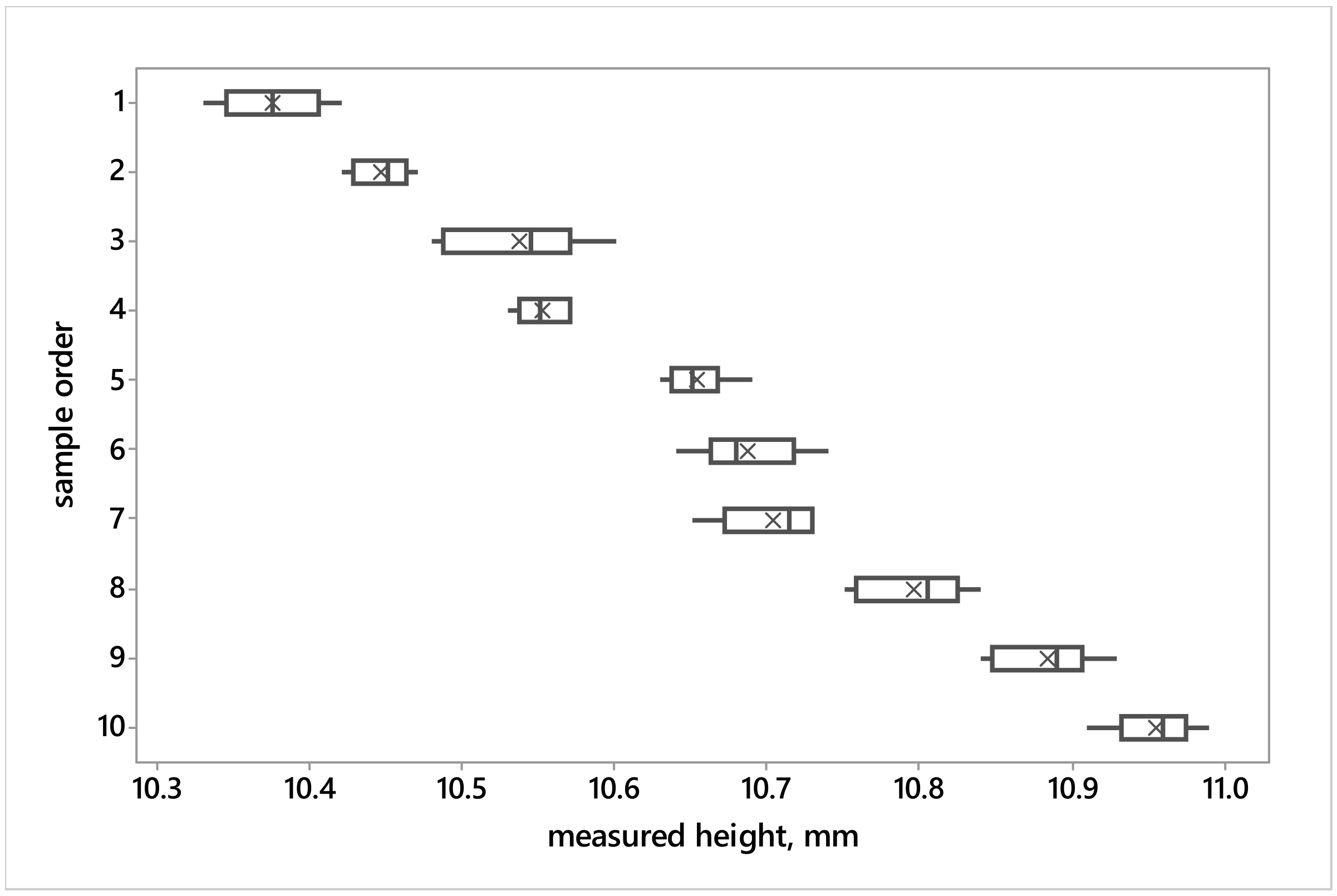
Figure 1 shows the box and whisker plots for each individual sample for the case when the samples are arranged in the original, random order. After sorting the samples according to the magnitude of average values (see Figure 2), the graph is much clearer, and it is also possible to roughly assess how the variability of the repeated measurements changes with the magnitude of the measured value (in this case, it is a variability caused by both the repeatability and reproducibility).

The application of box and whisker plots to real data shows that the measurements of individual samples do not contain any outliers. The analysis of Figure 2, with ordered samples, leads to the approximate conclusion that the variability of the measured values probably does not depend on the magnitude of the measured value.

4.2.2. The Scatter Plot of Individual Measurements and a Modified GRR Diagram

Another newly designed graphical tool is a scatter plot showing the individual measurements of an operator in relation to the overall average calculated from all the measurements of a given product sample (Figure 3a). The graph designed in this way allows one to assess the variability of individual measurements of a given operator and to compare them with the overall average. Thanks to the plotted line of the product sample averages, it is possible to assess whether any of the operators achieved larger deviations from these averages.

By analyzing Figure 3a, it can be concluded that the smallest variability of the repeated measurements is achieved by operator A. This operator’s measurements are also close to the sample average values. In contrast, operator B usually measures values above average, while operator C usually measures values lower than average.

The differences in the measurements of the individual operators can be displayed even more clearly using a modified “GRR diagram”. The GRR diagram is not included in the MSA manual, but it is used by some software products containing Gage R&R analysis. The version proposed by the authors of this paper (see Figure 3b) differs in that the samples are not arranged in random order; the individual product sample averages are plotted on the x-axis. Every point in the diagram shows the difference between the measurements of a specific product sample and the overall average of the sample. The horizontal full red lines correspond to differences between the averages of all product samples measured by individual operators and the total average of all measurements.

The analysis of Figure 3b, for example, confirms that the lowest measurement variability was achieved by operator A and that these measured values are the nearest to the average of all the measurements. It is also clear that operator B measures values that are above the overall average, and operator C measures values that are below the overall average. Regarding the fact that in this diagram overall average values of product samples are on the x-axis, the diagram also provides some information about the measurement system uniformity. In the given case, it can be estimated that the uniformity is acceptable because the variability of the repeated measurements apparently does not depend on the magnitude of the measured value.

A clear comparison of all individual measurements and the variability of the repeated measurements can be made in the next proposed modification of the GRR diagram (see Figure 4). In this diagram, for the individual product samples arranged by size, the deviations of the individual measurements taken by each operator from the sample averages are plotted. The analysis of the diagram suggests, for instance, rather different measurements taken by operator C in the case of the third, eighth and ninth samples compared to the other two operators, which can signal an effect of some particular cause on the measurement process. It would be desirable to identify and permanently eliminate this cause and repeat the measurements of the given samples.

If the behavior of one of the operators appears to be a possible cause of the unexpected measurement results, this can be assessed by a new analysis of the repeatability and reproducibility, this time excluding the data measured by the given operator [21]. Comparing the results obtained for the measurement system involving all operators versus the one involving only some operators can help reveal the weak points of the measurement system.

4.2.3. Range Control Chart

Before evaluating the repeatability and reproducibility of the measurement system, it is necessary to verify one of the assumptions: the statistical stability of the measurement process related to the variability of the repeated measurements. This verification is done by means of the range control chart (in fact, it is not the “true” control chart because the x-axis does not correspond to the time axis; in the original concept, the product sample numbers are on the x-axis).

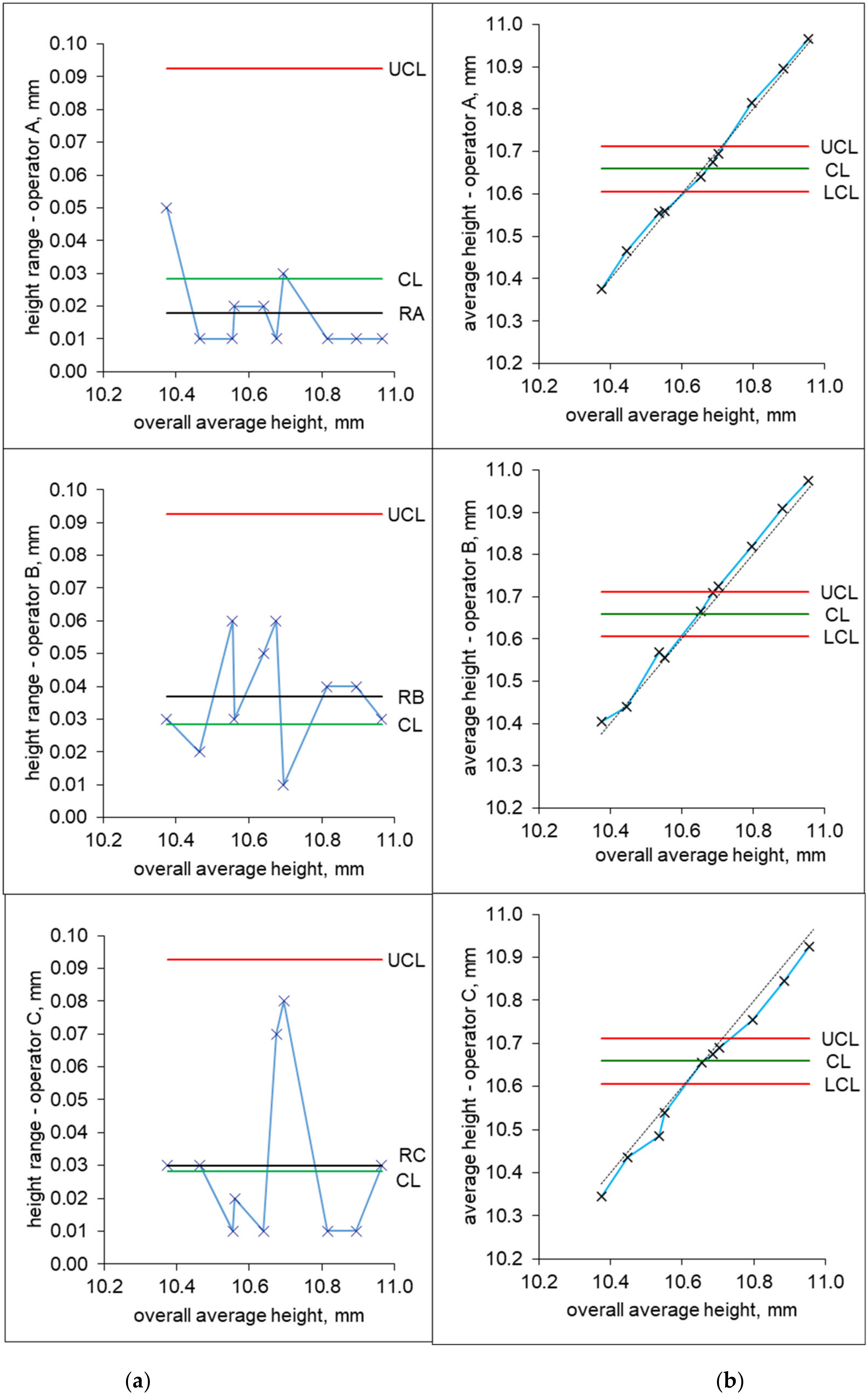
The authors’ proposal is to replace the sample numbers with the individual sample averages. This change, which does not affect the evaluation of the diagram, allows at least a qualitative assessment of the uniformity of the measurement system (independence of the repeatability of the measurement system on the magnitude of the measured value). The proposed diagram also shows the level of the average range of the repeated measurements for individual operators RA, RB and RC and allows their comparison (see Figure 5a).

The level of the control chart central line corresponds to the average range for all operators. The central line (CL), lower control limit (LCL) and upper control limit (UCL) are calculated according to the following formulas:

$$\mathrm{CL}=\overline{\mathrm{R}}=\frac{{\sum }_{\mathrm{i}=1}^{\mathrm{h}}{\overline{\mathrm{R}}}_{\mathrm{i}..}}{\mathrm{h}};\hspace{1em}\mathrm{LCL}={\mathrm{D}}_3\cdot \overline{\mathrm{R}};\hspace{1em}\mathrm{UCL}={\mathrm{D}}_4\cdot \overline{\mathrm{R}}$$

(6)

where ${\overline{\mathrm{R}}}_{\mathrm{i}..}$ denotes the operator-specific average range, h is the number of operators and D₃, D₄ are the coefficients dependent on the number of trials [22].

The subgroup size, for which it is necessary to find the coefficients D₃ and D₄, corresponds to the number of repeated measurements of each product sample [22]. The statistical stability is achieved when all plotted values are found within the control limits.

From Figure 5a, it is obvious that the analyzed measurement system is, regarding the variability of the repeated measurements, in control. A comparison of the average ranges calculated for the individual operators (RA, RB, RC) leads to the conclusion that the lowest variability of the repeated measurements is achieved by operator A. In contrast, operator B has an average range that is approximately two times higher. This finding should provide an impetus for a more detailed analysis of the causes of these differences and for finding appropriate improvement actions. Additionally, significant changes in the variability of the repeated measurements of operator C (see Figure 5a) should be analyzed in more detail.

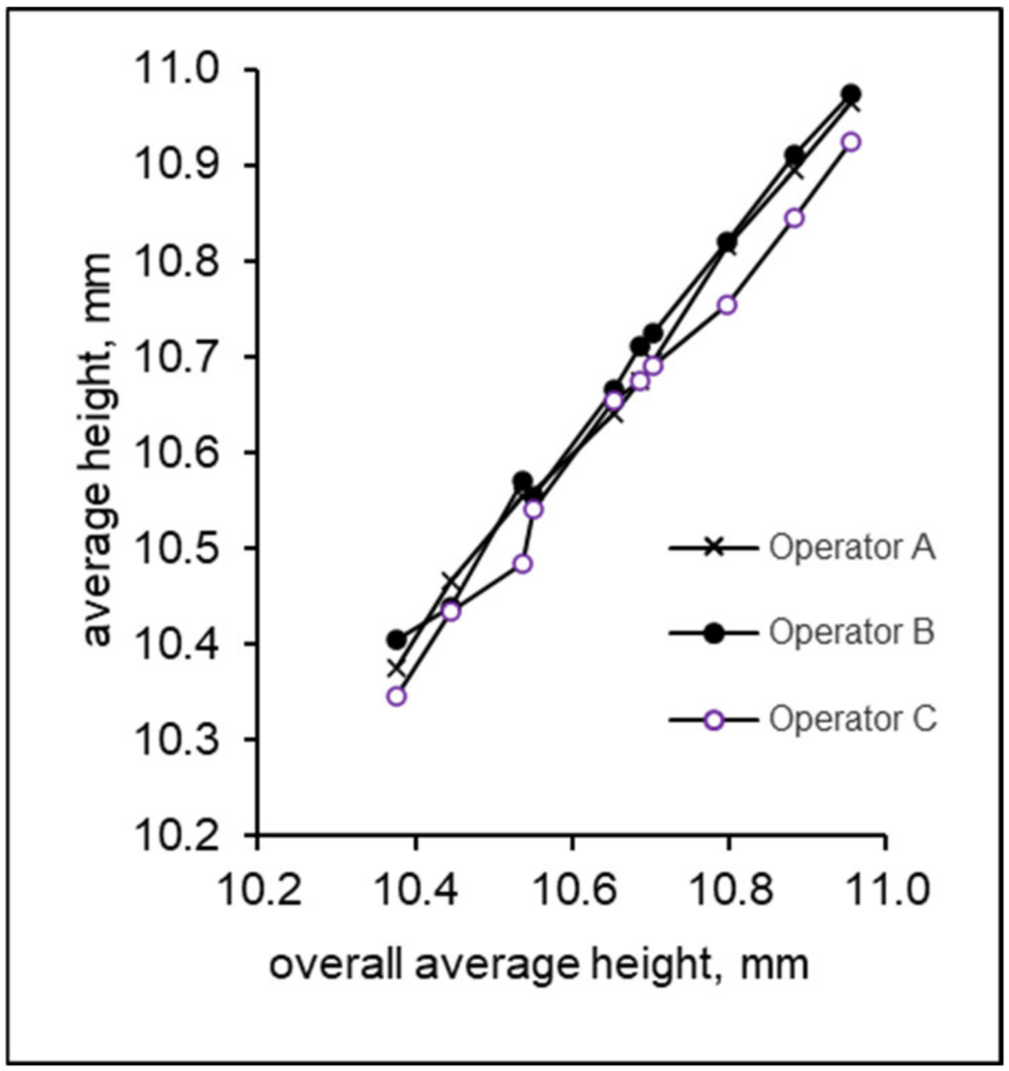
It can also be concluded that the variability of the repeated measurements does not depend on the magnitude of the measured value (conforming uniformity). Since the ranges of the repeated measurements fluctuate a great deal for some operators, an analysis of the dependence of the average range on the product sample average was performed (see Figure 6). This diagram confirms that the average variability of the repeated measurements does not seem to depend on the magnitude of the measured value.

4.2.4. Average Control Chart

The suitability of the measurement system for the evaluation of variability among the measured product samples is assessed by means of the average control chart. In this diagram, the averages calculated from the measurements of the individual product samples carried out by each individual operator are drawn. For better transparency, these averages shall be drawn separately for each operator. The central line (CL), lower control limit (LCL) and upper control limit (UCL) are calculated according to the following formulas:

$$\mathrm{CL}=\overline{\mathrm{x}}=\frac{{\sum }_{\mathrm{i}=1}^{\mathrm{h}}{\overline{\mathrm{x}}}_{\mathrm{i}..}}{\mathrm{h}};\hspace{1em}\mathrm{LCL}=\overline{\mathrm{x}}-{\mathrm{A}}_2\cdot \overline{\mathrm{R}};\hspace{1em}\mathrm{UCL}=\overline{\mathrm{x}}+{\mathrm{A}}_2\cdot \overline{\mathrm{R}}$$

(7)

where ${\overline{\mathrm{x}}}_{\mathrm{i}..}$ denotes the operator-specific average measurement, h is the number of operators and A₂ is the coefficient, depending on the number of trials [22].

Regarding the fact that the relevant control limits are defined by the variability given within the subgroups (they represent the variability of the measurement system), it cannot be expected that the values will be found within the control limits. The measurement system is considered as conforming to the evaluation of the variability among the measured samples if at least a half of the drawn averages are out of the control limits [2] (this rule cannot be used in the case when the product samples do not cover the production process variability). In this case, where product samples cover production process variability, Figure 5b shows that the analyzed measurement system is appropriate for the evaluation of variability among the measured samples, because 73% of the points lie outside the control limits.

This diagram is suitable even if the samples do not represent the production range, because it allows one to compare the average values of the measurements taken by the individual operators for the individual samples.

4.2.5. Interaction Plots

A certain modification of the average control chart is the stacked average chart, also called the operator–sample interaction plot. This diagram (see Figure 7) can be used for a clearer comparison of the operators’ average measurements taken for each product sample and for a basic assessment of a possible occurrence of operator–sample interactions. These interactions are a source of variability of the measurement system, and therefore it is desirable to identify them and eliminate their causes.

In the proposed modification of this diagram, the product sample average measurements are plotted on the x-axis instead of the product sample number. Non-parallel or crossed connections of individual points signal possible interactions.

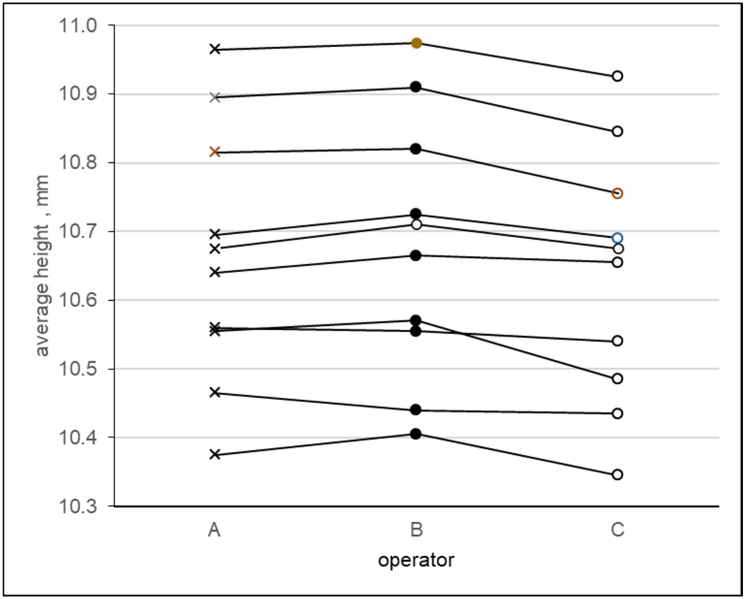
A weakness of this diagram is an occasional overlapping of the points in the case when different operators reach the same average measurement for some product samples. Because the measurement variability caused by different operators is usually always smaller than the variability of the measured product samples, the authors recommend graphical analysis of interactions using a diagram with different arrangement (see Figure 8). This diagram is much clearer, and its analysis can identify different slopes of point connections in the case of the second and fourth product samples, which can signal possible interactions between the operators and these samples.

To obtain even clearer graphical information about possible interactions between the operators and samples, a diagram of deviations of the averages achieved by the individual operators for the individual samples from the total average of all measurements of a given sample was proposed (see Figure 9).

The proposed diagram makes it possible to better evaluate the differences between the averages of repeated measurements of the individual operators calculated for the individual samples and to identify different slopes of the point connections. In this case, the course of the individual connections indicates possible interactions between the operators and samples in the case of the second, fourth and fifth samples.

All these graphical analyses of interactions provide only approximate information about possible interactions; however, they can be an impetus for an analysis and elimination of their causes. Numerically, the variability caused by interactions can be evaluated using ANOVA. In this case, ANOVA application leads to the conclusion that the component of variability caused by the interactions between the operators and samples is statistically insignificant at the significance level of α = 0.05.

5. Discussion

From the given examples of the use of the proposed graphical tools of Gage R&R analysis, it is evident that by applying them, more detailed information about the behavior of the analyzed measurement system can be obtained, and the causes of the variability of the measured values can be identified in more detail. This information is a valuable basis for the design and implementation of appropriate measures to improve the measurement system.

Evaluation of the repeatability and reproducibility of the given measurement system using ANOVA led to the following results: %EV = 12.95%; %AV = 11.14%; %GRR = 17.08%; %PV = 98.53%; ndc = 8. If we were to limit ourselves only to these numerical results, we can only state that the measurement system can be classified as “acceptable for some applications, it should be approved by the customer” and that repeatability–equipment variation contributes somewhat more to the overall variability of measurement system.

Only a detailed analysis of the measured data with the help of proposed graphical tools of Gage R&R analysis makes it possible to reveal the specific causes of the variability of the measurement system and implement appropriate measures to improve it.

6. Conclusions

In practice, gage repeatability and reproducibility analyses are processed with some spreadsheet applications or other software products. Graphical tools for measurement system analysis are not often available or are disregarded or ignored. However, their usage brings valuable information about the analyzed measurement system that cannot be read from the numerical analysis.

The article proposes new or modified graphical tools for analyzing the repeatability and reproducibility of a measurement system. These tools make it possible to clearly analyze measured values, identify causes of measurement system variability and evaluate some other properties. Their use should become a standard part of the repeatability and reproducibility analysis. The proposed graphical tools can significantly contribute to improving the measured data quality based on which important decisions are made. Further research will be focused on confirming the utility of the proposed graphical tools in improving various measurement systems.