Dynamically Coupled Reservoir and Wellbore Simulation Research in Two-Phase Flow Systems: A Critical Review

Abstract

A coupled reservoir/wellbore simulator is essential for solving relevant flow phenomena with dynamic interactions between reservoir and wellbore in two-phase flow systems. A reservoir simulator or wellbore simulator alone fails to solve these transient flow phenomena. This paper summarises a critical review of the coupled reservoir and wellbore simulation. First, a wide application of the drift-flux (DF) models to simulate gas–liquid flow in a wellbore model coupling to a reservoir model was discussed. Then, the mechanisms of the coupled reservoir/wellbore simulator in two-phase flow systems were discussed, including the reservoir modeling, wellbore modeling, and their coupling schemes. Various examples of representative coupled simulators were presented. Finally, some case studies were reported to reveal dynamic interactions between wellbore and reservoir by using the coupled reservoir/wellbore simulators. This study gives the most up-to-date and systematic sights on the relevant research topic of reservoir/wellbore coupling, allowing for a better understanding of the coupled reservoir and wellbore simulation and its application in the oil and gas industry.

1. Introduction

The dynamic interaction between wellbore and reservoir research is essential to solve transient flow problems, such as wellbore storage, gas lift, coning, near-well cleanup, liquid loading, slugging, shut-in, start-up, smart wells, and reservoir management and forecast [1,2]. In multi-phase (gas, water, and oil) flow, the pore saturation and temperature and pressure propagation changes in a reservoir respond to propagation ranging timescales from hours to decades. Moreover, the wellbore’s multi-phase flow, temperature, and pressure propagation have response times from seconds to hours. The dynamic dispatch between the wellbore and reservoir leads to results in production instabilities, which can deteriorate the reservoir and wellbore production lifespan and ultimate recovery [3]. Figure 1 provides a summary of common transient flow issues between reservoir and wellbore.

Most wellbore simulators are employed to solve the flow issues in the wellbore area, whereas the reservoir simulators are used to simulate the reservoir phenomena. These simulations apply either a dynamic reservoir model coupled with a steady wellbore model [5,6,7,8] or a dynamic wellbore model coupled with an analytical reservoir model [9,10,11]. Moreover, most commercial reservoir simulators (e.g., Eclipse and CMG) use steady-state values of bottom hole pressure (BHP) and tubing head pressure (THP). Similarly, most commercial wellbore flow simulators (e.g., PIPESIM and Prosper) assume a given multi-phase fluid flow rate from a reservoir into a wellbore for a reservoir pressure and constant BHP [12] (Holmes et al., 1998). These commercial simulators do not square up a significant separation in spatial and time scales between reservoir and wellbore simulations. These models disregard the dynamic interactions between the wellbore and reservoir, resulting in erroneous simulation predictions.

In the past few years, some parties and scholars realized the importance of the dynamic interactions between wellbore and reservoir and have been working on the development and application of wellbore-reservoir simulators. Millier [13] might be the earliest scholar who studied transient interactions between wellbore and reservoir for well testing in geothermal wells. Other coupled reservoir/wellbore simulators were established to simulate dynamic flow problems between reservoirs and wellbores [1,3,14,15,16,17,18,19,20,21,22,23,24,25,26,27,28,29,30,31,32,33,34,35]. Numerical wellbore simulation contains a mass equation, momentum equation, and energy equation [36,37]. Darcy’s law is widely used to replace the classic momentum equation in reservoir simulation. In addition, most reservoir simulations suppose an iso-thermal condition, which implies that the energy equation is unnecessary [38,39]. Coupled reservoir/wellbore simulations combine the coupling of the reservoir’s partial differential equations (PDEs) and wellbore’s PDEs. Three different coupling schemes (explicit, implicit, and fully implicit) are widely applied to construct dynamic reservoir/wellbore simulators [40]. The researchers mentioned above suggested their coupling models resolve specific flow problems between the reservoir and wellbore.

In this paper, we critically reviewed numerical simulations of wellbore and reservoir models described in the open literature. While this review may not necessarily mention all the existing models, it was ensured that a representative set of publications are covered. The prospect of this review paper was to help researchers quickly understand the mechanisms of reservoir/wellbore coupling and further improve its application.

We discussed the application of the drift-flux (DF) models for coupled reservoir-wellbore simulation in Section 2. Then, in Section 3, reservoir modeling, wellbore modeling, and their coupling schemes are described. Following that, a number of significant complexities of coupled reservoir/wellbore simulators are discussed in Section 4. Finally, Section 5 provides a summary of the findings.

2. The Drift-Flux Model

2.1. Role of Drift-Flux Models

There are huge differences in the definitions of phase velocities between wellbore and reservoir simulations. As is often the case, the phase velocities in a reservoir are usually small, with negligible kinetic energy, for which Darcy’s law is applicable to calculate the phase velocities [41]. However, the kinetic energy must be considered in a wellbore simulation. The phase velocities are determined by the gas–liquid two-phase momentum equations [36]. The earliest model applied an empirical mixture equation to describe the two-phase flow [42,43,44,45,46]. More complex models considered homogeneous flow, separated flow, and DF flow to simulate the two-phase momentum conservation. In the early 1980s, separate flow models were used for coupled numerical reservoir/wellbore systems [14,26]. Holmes et al. [12] outlined a multisegment well model to simulate gas–liquid flow in advanced wells. Two case studies of a horizontal well and a dual-lateral well were implemented to evaluate the performance of their multisegment well model. It was one of the first attempts to use a DF model to simulate the gas–liquid flow in a wellbore, rather than using traditional separated models [12]. As early as 1977, Holmes [47] proposed his research to use the DF model to simulate flow rates of individual liquid or gas phases. After Holme’s publication, most of the subsequent researchers implemented DF models for coupled reservoir/wellbore research [48,49,50,51,52,53] Homogeneous (no-slip) models can also be used for coupled reservoir/wellbore simulations, but they fail to accurately calculate in situ phase volume fractions and input volume fractions. Separate models need more computational requirements considering separate conservation equations for liquid and gas phases. Furthermore, the separate models result in discontinuous flow rates or discontinuous derivatives of flow rates due to the existence of the discrete flow regimes [2], which limits the application of these separate models for coupled reservoir/wellbore simulations. Conversely, DF models are considered accurate in predicting gas volume fractions in gas–liquid flow [54]. Tang et al. summarized two essential prerequisites for fully implicitly coupled reservoir/wellbore simulators [53]. One is a mixture velocity for the gas or liquid phase, and the other is that the model must be continuous and differentiable. In general, a DF model is suitable for strongly coupling reservoir/wellbore simulators. More follow-up studies will apply DF models to simulate the gas–liquid flow in the wellbore coupling to the reservoir.

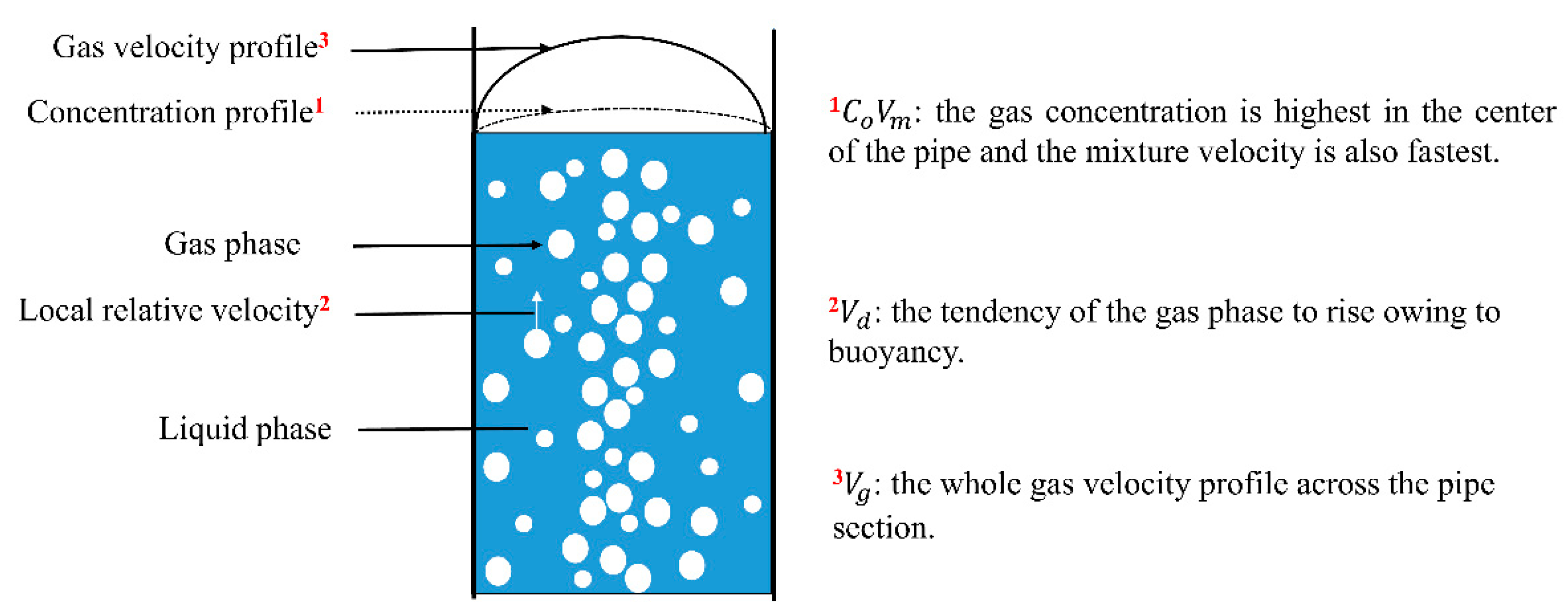
2.2. Description of a Basic DF Model

The DF models have been widely applied in the nuclear industry for a while [55,56,57,58]. As indicated above, since Holmes [12] extensively applied a DF model for reservoir simulation, the use of DF models to couple the wellbore flow to a reservoir has been a common practice. The DF models consider the slip between fluid and gas phases, and they are continuous and differentiable, making them suitable for coupling reservoir/wellbore simulations.

The basic DF model was first proposed by Zuber and Findlay [59]. This one-dimensional DF model describes the slip effect between the gas and liquid phases. The general formulation is expressed in Equation (1):

$$V_{\mathrm{g} }{=C}_{\mathrm{o}}{V}_{\mathrm{m}}{ + V}_{\mathrm{d}}$$

(1)

where V_g is the flow velocity of the gas phase; C_o is a profile parameter that reveals the effect of a non-uniform flow profile over a pipe cross-section; V_m is an average velocity of the mixture; V_d is the drift velocity considering the slip between the gas and liquid phases. V_m can be defined:

$$V_{\mathrm{m}}{=V}_{\mathrm{sg}}{ + V}_{\mathrm{sl}}{ = V}_{\mathrm{g}}{\alpha }_{\mathrm{g}}{+V}_{\mathrm{l}}{(1 - \alpha }_{\mathrm{g}})$$

(2)

where V_sg is the gas superficial velocity; $V_{\mathrm{sl}}$ is the liquid superficial velocity; $V_{\mathrm{l}}$ is the flow velocity of liquid; ${\alpha }_{\mathrm{g}}$is the in situ gas volume fraction.

Figure 2 summarizes the mechanism of the basic DF model. The gas velocity is illustrated by a combination of the differences in gas concentration across the pipe section and the tendency of the gas phase to rise in the tubing due to buoyancy [50,60,61].

DF models require some empirical parameters. However, most of these parameters must be determined by experiments in vertical pipes with 2 inches or smaller diameters. These parameters can not be applicable in wellbore two-phase flow due to the huge differences in flow mechanisms between different large pipes and small pipes [62]. Therefore, the overall goal is to form unified drift-flux models for coupled reservoir/wellbore simulators by adjusting these empirical parameters.

Since first published in 1965, the basic DF model has been refined by many researchers. In an early application in thermal-hydraulic analysis, Coddington and Macian [63] presented a good review of 13 DF correlations to accurately forecast rod bundle void fractions in a nuclear reactor core. They summarized all the expressions of these correlations, showing that they can perform well for a broad range of experimental conditions [59,64,65,66,67,68,69,70,71,72,73,74]. For the oil and gas industry, since Holmes [12] published his work on an application of a drift-flux model in advanced wells, Hasan and Kabir [75,76,77] and Ansari et al. [78] improved their DF correlations, and these models are widely used for gas–liquid flow modeling in pipes [36,79,80,81]. However, only a very limited number of DF models were proven to be suitable for coupled reservoir/wellbore systems [47,60,61,82,83].

2.3. Unified Gas/Liquid DF Models for Coupled Reservoir/Wellbore Simulators

One of the most widely applicable DF models for coupled reservoir/wellbore simulations was proposed by Shi et al. [60,61]. Their model could simulate concurrent and countercurrent flows, as well as complex advanced wells. They covered and improved the DF model first presented by Homes [47]. Oddie et al. [84] performed large-scale flow experiments for multi-phase flows at various inclinations to determine these empirical parameters in Shi et al.’s model. Livescu et al. [20,49,50] and Semenova et al. [85] implemented this DF model, which was applied to Stanford’s General Purpose Research Simulator, detailed in Cao [86] and Jiang [87]. Shi et al.’s model was also applied in other coupled reservoir/wellbore simulators and commercial simulators [21,48,51,88]. However, this model is suitable only for a pipe inclination from +2° (near horizontal) to +90°(vertical upward), which thereby limits its application. Figure 3 summarizes the use of multiplier m(θ) to compensate for gas/liquid deviation in Shi et al.’s model. It covered Hasan and Kabir’s [77] multiplier m(θ) and refined a valid range for θ from [2°, 30°] to [2°, 90°]. A solution for the multiplier m(θ) for the gray region (θ ∈ [0°, 2°]) has not been yet posed. As a DF model was developed from near-horizontal and vertical flow, it remained unsuited for horizontal or downward flow.

With an extensive application of horizontal wells and undulating horizontal wells, there is a need to extend the inclination range of Shi et al.’s DF model [89,90,91]. Li et al. [92] presented a simple stratified equivalent model to extend Shi’s model from −5° (downward flow) to +90°, and their model is suitable for complex coupled systems. Choi et al. [93] raised an efficient DF model to forecast liquid holdups in a broad range of pipeline inclination angles. Choi et al.’s [93] model was verified using an experimental dataset from Tulsa University Fluid Flow Projects (TUFFP) and a synthetic dataset from OiL and GAs simulator (OLGA) by the SPT group with inclination ([−30°, 90°]). A subsequent DF model proposed by Bhagwat and Ghajar [94] represented the widest range of inclination (θ ∈ [−90°, 90°]). The correlation of Bhagwat and Ghajar’s model had a significant performance on the entire range of void fractions. However, all these DF models were never applied in wellbore two-phase flow for coupling to a reservoir model. Other representative DF models suitable for coupled reservoir/wellbore simulators were developed by Tang et al. [82,83,95]. First, Tang et al. [95] extended Shi et al.’s model to horizontal flow to simulate the liquid loading phenomenon in horizontal wells. Then, Tang et al. [82,83] developed a unified DF model for all wellbore inclinations (θ ∈ [−90°, 90°]). Two datasets from TUFFP and OLGA-S were used to determine optimal parameters in Tang et al.’s model.

Table 1. Summary of datasets from TUFFP used for parameters optimization in Tang et al.’s model.

Time	Author	Inclination, θ (degrees)	Pipe Diameter, D (cm)	Gas Superficial Velocity, Vg (m/s)	Liquid Superficial Velocity, VL (m/s)
1967	Eaton [99].	0	10.20	[0.112, 21.901]	[0.011, 2.108]
1972	Beggs [100]	[−10, 10]	2.54	[0.299, 25.323]	[0.023, 5.203]
1976	Schmidt [101]	90	5.08	[0.042, 13.146]	[0.070, 2.146]
1977	Cheremisinoff [102]	0	6.35	[2.582, 25.241]	[0.017, 0.070]
1980	Mukherjee [103]	[−90, 90]	3.81	[0.037, 41.310]	[0.015, 4.362]
1980	Akpan [104]	0	7.62	[0.199, 5.458]	[0.137, 1.701]
1982	Vongvuthipornchai [105]	0	7.62	[0.061, 2.938]	[0.070, 2.146]
1983	Minami [106]	0	7.79	[0.475, 16.590]	[0.005, 0.951]
1986	Caetano [107]	90	6.34	[0.023, 22.859]	[0.002, 3.579]
1986	Kouba [108]	0	7.62	[0.302, 7.361]	[0.152, 2.137]
1986	Rothe et al. [109]	[−2, 0]	17.10	[0.610, 4.633]	[0.061, 1.830]
1992	Felizola [110]	[0, 90]	5.10	[0.390, 3.360]	[0.050, 1.490]
1996	Roumazeilles [111]	[−30, 0]	5.10	[0.914, 9.357]	[0.884, 2.438]
1996	Brill et al. [112]	[−10, 10]	7.79	[3.629, 12.656]	[0.004, 0.046]
1999	Meng [113]	[−2, 2]	5.08	[4.600, 26.600]	[0.001, 0.054]
2000	Abdul-Majeed [114]	0	5.08	[0.196, 49.908]	[0.002, 1.825]
2005	Fan [115]	[−2, 2]	5.08	[4.930, 25.700]	[0.0003, 0.052]
2005	Johnson [116]	[0, 5]	10.00	[0.711, 4.523]	[0.019, 0.605]
2009	Magrini [117]	[0, 90]	7.62	[36.630, 82.320]	[0.003, 0.040]
2011	Yuan [118]	[30, 90]	7.62	[9.900, 36.000]	[0.005, 0.100]
2012	Guner [119]	[0, 45]	7.62	[1.485, 39.388]	[0.010, 0.100]
2013	Alsaadi [120]	[2, 30]	7.62	[1.829, 39.992]	[0.010, 0.101]

summarizes all the public sources from TUFFP [96], which can be worthy for subsequent new DF models. Tang et al. [28,53,82,83,95,96] implemented their DF model into the General Unstructured Reservoir Utility (GURU) at Texas A&M University, detailed in Yan [97] and Olivares [98].

We reviewed several DF models for simulating gas–liquid flow in the wellbore at various inclinations. Shi et al.’s model was regarded as the DF model with the widest application for coupled reservoir/wellbore simulators. Tang et al. claimed that their model was unified and suitable for any coupled systems, whereas other DF models have the potential to be applied in coupled reservoir/wellbore simulators in future work.

Table 2. Several unified DF models for coupled reservoir/wellbore simulation.

Author	Inclination θ (Degrees)	Correlation
Shi et al. [60,61]	[+2, +90]	$C_{\mathrm{o}}=\frac{A}{1 + \left(A - 1\right){\gamma }^2}$ $V_{\mathrm{d}}=\frac{{(1 - \alpha }_{\mathrm{g}}{C}_{\mathrm{o}}{)C}_{\mathrm{o}}{K(\alpha }_{\mathrm{g}}{)V}_{\mathrm{C}}}{{\alpha }_{\mathrm{g}}{C}_{\mathrm{o}}\sqrt{\frac{{\rho }_{\mathrm{g}}}{{\rho }_{\mathrm{l}}}}{ + 1 - \alpha }_{\mathrm{g}}{C}_{\mathrm{o}}}$
Li et al. [121]	[−5, +90]	${\alpha }_{\mathrm{g}}=\frac{V_{\mathrm{g}}{\alpha }_{\mathrm{g}}}{C_{\mathrm{o}}\left({\alpha }_{\mathrm{g}}{, X}_{\mathrm{p}}\right)V_{\mathrm{m}}{ + V}_{\mathrm{d}}{(\alpha }_{\mathrm{g}}{, X}_{\mathrm{p}})}$ ${\alpha }_{\mathrm{g}}\left(\theta \right){=C}_1\left(\theta \right){\left({\alpha }_{\mathrm{g}}\right)}^{\mathrm{SE}}{ + [1 - C}_1\left(\theta \right)]{\left({\alpha }_{\mathrm{g}}\right)}^{\mathrm{DF}}$ $C_1\left(\theta \right)=\{\begin{array}{c}1 \mathrm{for} \theta ϵ{ [\theta }^{\mathrm{SE}}{, 0}^{\text{°}}]\\ \exp \left(-\beta \frac{{\theta }^2}{{\left({\theta }^{\mathrm{DF}}\right)}^2{ - \theta }^2}\right) \mathrm{for} \theta ϵ{ [0}^{\text{°}}{, \theta }^{\mathrm{DF}}] \\ 0 \mathrm{for} \theta ϵ{ [\theta }^{\mathrm{DF}}{, 90}^{\text{°}}] \end{array}$
Choi et al. [93]	[−30, 90]	$C_{\mathrm{o}}=\frac{2}{1 + {\left(\mathrm{Re}/1000\right)}^2}+\frac{1.2 - 0.2\sqrt{\frac{{\rho }_g}{{\rho }_l}}{(1 - \exp (-18\alpha }_{\mathrm{g}}\left)\right)}{1+{\left(1000/\mathrm{Re}\right)}^2}$ $V_{\mathrm{d}}=A\cos \theta +B(\frac{\mathrm{g}\mathsf{\sigma }\mathsf{\Delta }\rho }{{\rho }_l{}^2}{)}^{1/4}\sin \theta$
Bhagwat and Ghajar [94]	[−90, 90]	$C_{\mathrm{o}}=\frac{{2 - (\rho }_{\mathrm{g}}{/\rho }_{\mathrm{l}}{)}^2}{1+{\left(\mathrm{Re}/1000\right)}^2}+\frac{{\left[\right(\sqrt{(1 + {\left(\frac{{\rho }_{\mathrm{g}}}{{\rho }_{\mathrm{l}}}\right)}^2\cos \theta \left)\right)/(1 + \cos \theta )}{)}^{(1 - \alpha )}]}^{2/5}{ + C}_{0.1}}{1 + {\left(1000/\mathrm{Re}\right)}^2}$ $V_{\mathrm{d}}=(0.35\sin \theta +0.45\cos \theta ) \times \sqrt{\frac{\mathrm{g}D\left({\rho }_{\mathrm{l}}{ - \rho }_{\mathrm{g}}\right)}{{\rho }_{\mathrm{l}}}}\left({1 - \alpha }_{\mathrm{g}}\right)C_2{C}_3{C}_4$ $C_{0.1}=\{\begin{array}{c}{0, -50}^{\text{°}}\le \theta \le { 0}^{\text{°}}{ \mathrm{and} Fr}_{\mathrm{sg}} \le 0.1\\ {(C}_1{ - C}_1\sqrt{\frac{{\rho }_{\mathrm{g}}}{{\rho }_{\mathrm{l}}}}\left)\right[{\left(2.6 - \beta \right)}^{0.15} - \sqrt{f_{\mathrm{tp}}}{](1 - x)}^{1.5}, \mathrm{otherwise}\end{array}$ $C_2=\{\begin{array}{c}{[\frac{0.434}{{\log (\mu }_{\mathrm{l}}/0.001)}]}^{0.15}{, (\mu }_{\mathrm{l}}/0.001) > 10 \\ {1 , (\mu }_{\mathrm{l}}/0.001) \le 10\end{array}$ $C_3=\{\begin{array}{c}(L\mathrm{a}/0.025{)}^{0.9}, L\mathrm{a} > 0.025 \\ 1 , L\mathrm{a} \le 0.025\end{array}$ $C_4=\{\begin{array}{c}{-1, -50}^{°}\le \theta \le { 0}^{°}{ \mathrm{and} Fr}_{\mathrm{sg}} \le 0.1 \\ 1, \mathrm{otherwise}\end{array}$
Tang et al. [53]	[0, 90]	$C_{\mathrm{o}}=\frac{A}{1+\left(A - 1\right){\gamma }^2}$ $V_{\mathrm{d}}=\frac{{(1 - \alpha }_{\mathrm{g}}{C}_{\mathrm{o}}{)C}_{\mathrm{o}}{\mathrm{m}V}_c}{{\alpha }_{\mathrm{g}}{C}_{\mathrm{o}}\sqrt{\frac{{\rho }_{\mathrm{g}}}{{\rho }_{\mathrm{l}}}}{+1 - \alpha }_{\mathrm{g}}{C}_{\mathrm{o}}}, 0^{°}\le \theta \le 2^{°}$ $V_C=\sqrt{\frac{{\mathrm{g}D(\rho }_{\mathrm{l}}{ - \rho }_{\mathrm{g}})}{{\rho }_{\mathrm{l}}}}$ $V_{\mathrm{d}}=\frac{{(1 - \alpha }_{\mathrm{g}}{C}_{\mathrm{o}}{)C}_{\mathrm{o}}{K(\alpha }_{\mathrm{g}}{)V}_C}{{\alpha }_{\mathrm{g}}{C}_{\mathrm{o}}\sqrt{\frac{{\rho }_{\mathrm{g}}}{{\rho }_{\mathrm{l}}}}{+1 - \alpha }_{\mathrm{g}}{C}_{\mathrm{o}}}, 2^{°}\le \theta \le {90}^{°}$ $V_{dm}=V_d\times m\times f\left(\theta \right)$
Tang et al. [82,83]	[−90, 90]	$C_{\mathrm{o}}=\frac{A}{1+(A - 1) \times \min \left\{{[\frac{\max \left({\alpha }_{\mathrm{g}},\frac{{\alpha }_{{\mathrm{g}|V}_{\mathrm{m}}|}}{V_{\mathrm{sgf}}}\right) - \mathrm{B}}{1 - \mathrm{B}}]}^2,1\right\}}$ $V_{\mathrm{d}}{=(m}_1{V}_{\mathrm{d}}{}^{\mathrm{V}}\sin \theta +\left\{1 - \frac{2}{{1+\exp [50 \times \times \sin (\theta +m}_2{V}_{\mathrm{m}})]}\right\}{V}_{\mathrm{d}}{}^{\mathrm{h}}\cos \theta )\times$ ${(1+\frac{1000}{{Re}_{\mathrm{l}}+1000})}^{m^3}$

presents the correlations of those advanced DF models discussed above.

Where${ C}_{\mathrm{o}}$ is the profile parameter;$V_{\mathrm{d}}$ is the drift velocity;$A$ is the value of the profile parameter in the bubble and slug flow regimes; $\gamma$ is the term involving to cause $C_{\mathrm{o}}$ to reduce to 1.0; ${\alpha }_{\mathrm{g}}$ is the in situ gas volume fraction; ${K(\alpha }_{\mathrm{g}})$ is the critical Kutateladze number; $V_C$ is the characteristic velocity. ${ X}_{\mathrm{p}}$ is the DF model parameter vector;$C_1\left(\theta \right)$ is the tunable weight function; $V_{\mathrm{g}}$ is the in situ gas velocity;$V_{\mathrm{m}}$ is the mixture velocity.$\theta$ is the pipe inclination angle; $\mathrm{Re}$ is the Reynolds number; $\mathsf{\sigma }$ is the surface tension; $\mathrm{A}, \mathrm{B}$ are the coefficient constant. ${Fr}_{\mathrm{sg}}$is the Froude number; $C_{0.1}$, C₂, C₃, C₄ are the coefficient constant;${ f}_{\mathrm{tp}}$ is the friction factor; ${\mu }_{\mathrm{l}}$ is the liquid viscosity; $L\mathrm{a}$ is the Laplace variable.$m$ is the coefficient constant; $f\left(\theta \right)$ represents the influence of pipe inclination; $V_{dm}$ is the modified $V_{\mathrm{d}}$. $V_{\mathrm{sgf}}$ is the gas flooding velocity; $m_1, m_2, m_3$are the coefficient constant; $V_{\mathrm{d}}{}^{\mathrm{V}}$ is the vertical drift velocity; $V_{\mathrm{d}}{}^{\mathrm{h}}$ is the horizontal drift velocity.

3. Coupled Reservoir/Wellbore Modeling

3.1. Reservoir Modeling

The numerical simulation of reservoir flow is based on a series of conservation equations, where typical variables are pressure and phase saturations [41]. Darcy’s law was selected to describe fluid velocities through porous media in the reservoirs. Hydrocarbons in a reservoir were described by using black oil or compositional models. Other auxiliary equations involve interfacial tensions and capillary effects. For example, we considered three-phase Darcy flow in the porous media in the compositional system. Equations (3) and (4) express the mass conservation equations for hydrocarbon components and the water phase [49,50,82,83]. Usually, hydrocarbon components are not present in the water phase. Equation (5) is the total energy balance equation.

$$\nabla \left[kA(\frac{k_{\mathrm{ro}}}{{\mu }_{\mathrm{o}}}{x}_{\mathrm{c}}{\tilde{\rho }}_{\mathrm{o}}\nabla \left(P_{\mathrm{o}} - {\rho }_{\mathrm{o}}gz\right) + \frac{k_{\mathrm{rg}}}{{\mu }_{\mathrm{g}}}{y}_{\mathrm{c}}{\tilde{\rho }}_{\mathrm{g}}\nabla \left(P_{\mathrm{g}} - {\rho }_{\mathrm{g}}gz\right))\right] = V_b\frac{\partial }{\partial \mathrm{t}}\left(\varphi \left(S_{\mathrm{o}}{x}_{\mathrm{c}}{\tilde{\rho }}_{\mathrm{o}}+S_{\mathrm{g}}{y}_{\mathrm{c}}{\tilde{\rho }}_{\mathrm{g}}\right)\right) - n_{\mathrm{c},\mathrm{s}}$$

(3)

$$\nabla \left[kA\frac{k_{rw}}{{\mu }_{\mathrm{w}}}{\tilde{\rho }}_{\mathrm{w}}\nabla \left(P_{\mathrm{w}} - {\rho }_{w}gz\right))\right] = V_{\mathrm{b}}\frac{\partial }{\partial \mathrm{t}}\left(\varphi \left(S_{\mathrm{w}}{\tilde{\rho }}_{\mathrm{w}}\right)\right) - n_{\mathrm{w},\mathrm{s}}$$

(4)

$$\nabla \left[kA{{\displaystyle \sum }}_{\alpha }{H}_{\alpha }\frac{k_{\mathrm{r}\alpha }}{{\mu }_{\alpha }}{\tilde{\rho }}_{\alpha }\nabla \left(P_{\alpha } - {\rho }_{\alpha }gz\right)\right] = V_{\mathrm{b}}\frac{\partial }{\partial \mathrm{t}}\left(\varphi {{\displaystyle \sum }}_{\alpha }{S}_{\alpha }{\tilde{\rho }}_{\alpha }{U}_{\alpha }\right) + Q_{loss} + q_H$$

(5)

where k is the absolute permeability; $V_{\mathrm{b}}$ is the bulk rock volume; $K_{r\alpha }(\alpha =o, g, w)$ is the phase relative permeability; $u_{\alpha }(\alpha =o, g, w)$ is the phase viscosity; A is a cross-sectional area; $P_{\alpha }(\alpha =o, g, w)$ is phase pressure; ${\tilde{\rho }}_{\alpha }(\alpha =o, g, w)$ is the molecular density; ${\rho }_{\alpha }(\alpha =o, g, w)$ is the mass density; g is the gravitational acceleration; z is the depth; $\varphi$ is the porosity; x_c and y_c are the mole fractions of hydrocarbon component c in the oil and gas phases, respectively; $S_{\alpha }(\alpha =o, g, w)$ is a phase saturation; n_c,s is a sink term; n_w,s is a source term; $H_{\alpha }(\alpha =o, g, w)$ is the enthalpy of the phase; $U_{\alpha }(\alpha =o, g, w)$ is the specific internal energy of the phase; $Q_{loss}$ represents the heat exchange between the reservoir and wellbore; $q_H$ is the internal source terms for the total energy.

These partial differential equations (PDEs) are usually resolved by a fully implicit time discretization and a finite-volume space discretization, although sometimes a finite element discretization is used in space [2,99,122]. An adaptive time-stepping scheme can also be applied for reservoir simulation. In a compositional simulation, the fluid properties of gas and oil phases are determined by vapor–liquid flash calculations based on an equation of state (EOS).

3.2. Wellbore Modeling

Numerical simulation of wellbore flow is based on a set of mass, momentum, and energy conservation equations. The mass conservations for hydrocarbons and water in wellbore flow are shown in Equations (5) and (6) [49,50,82,83]. The primary variables consist of hydrocarbon component molar fractions, pressure, volumetric holdups, and a mixture velocity. The superficial velocity phases in Equations (6) and (7) are determined by a DF model discussed in Section 2. By considering the case of two-phase flow, a momentum conservation equation for a pressure drop was obtained [123]. Equation (8) represents the total pressure loss for the whole wellbore [36,49,80,124]. The pressure drop equation consists of the pressure losses due to gravity, acceleration, and frictional effects. Equation (9) represents the total energy balance for the whole wellbore system. In thermal reservoir/wellbore simulators, the energy conservation equation is used to calculate temperature [15,36,125,126,127,128]. Moreover, the phase-equilibrium equations are chosen to calculate each phase’s mole fractions and composition under specific pressure and temperature conditions.

$$\nabla \left[A\right(x_c{\stackrel{\sim }{\rho }}_{\mathrm{o}}{v}_{so}+y_c{\stackrel{\sim }{\rho }}_{\mathrm{g}}{v}_{sg}=V_{\mathrm{seg}}\frac{\partial }{\partial \mathrm{t}}({\alpha }_{\mathrm{o}}{x}_c{\stackrel{\sim }{\rho }}_{\mathrm{o}}+{\alpha }_{\mathrm{g}}{y}_c{\stackrel{\sim }{\rho }}_{\mathrm{g}})+n_{c,s}$$

(6)

$$\nabla [A{\stackrel{\sim }{\rho }}_{\mathrm{w}}{v}_{sw}=V_{\mathrm{seg}}\frac{\partial }{\partial \mathrm{t}}({\alpha }_w{\stackrel{\sim }{\rho }}_{\mathrm{w}})+n_{w,s}$$

(7)

$$\frac{\partial P}{\partial z}+\frac{\partial {\rho }_{\mathrm{m}}{V}_{\mathrm{m}}{}^2}{\partial z}+\frac{f_{\mathrm{tp}}{\rho }_{\mathrm{m}}{V}_{\mathrm{m}}\left|V_{\mathrm{m}}\right|}{2d}{+\rho }_{\mathrm{m}}g\mathrm{gcos}\theta =0$$

(8)

$$\frac{\partial }{\partial z}{{\displaystyle \sum }}_f{\tilde{\rho }}_f{\alpha }_f\left(U_f+\frac{1}{2}{V}_f{}^2\right)+\frac{\partial }{\partial z}{{\displaystyle \sum }}_f{\tilde{\rho }}_f{V}_{sf}\left(H_f+\frac{1}{2}{V}_f{}^2\right)={{\displaystyle \sum }}_f{\tilde{\rho }}_f{V}_{Sf}g\cos \theta +Q_{loss}+q_H$$

(9)

where ${\alpha }_f (f=o, g, w)$ is the volumetric holdup; $v_f (f=o, g, w)$ is the superficial velocity; ${\rho }_{\mathrm{m}}$ is the mixture density; $v_{\mathrm{m}}$ is the average mixture velocity; d is the pipe inner diameter; $f_{\mathrm{tp}}$ is the friction factor;$H_f(f=o, g, w)$ is the phase enthalpy; $U_f(f=o, g, w)$ is the phase specific internal energy.

These PDEs of mass and momentum conservation equations can be one-dimensional, usually discretized in space by the finite-volume methods along the axial direction of a wellbore. Usually, a staggered grid arrangement is adopted for the discretization in space, which means that the variables of pressure, temperature, and holdup are calculated at the center of each segment while the velocities are solved at the face of each segment [20,82,83,122].

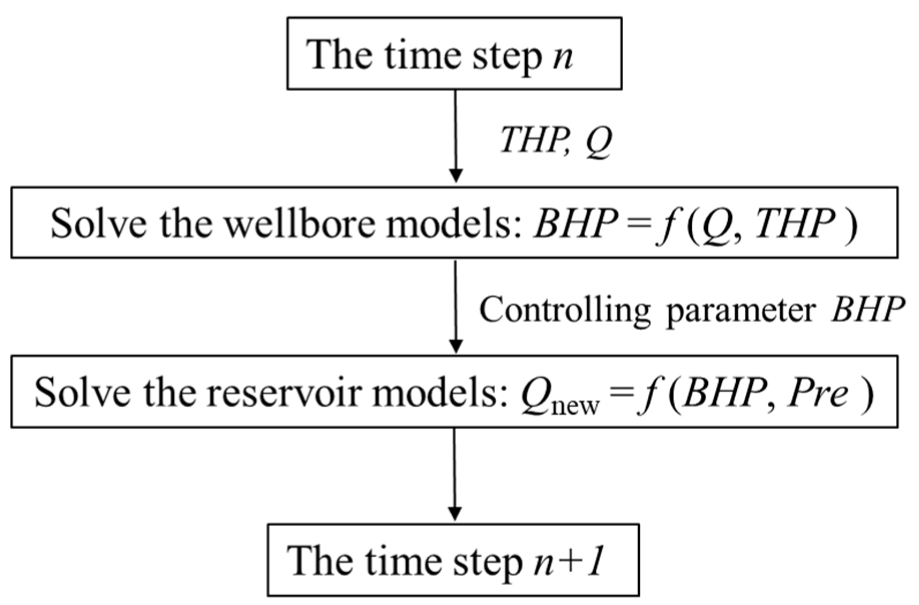
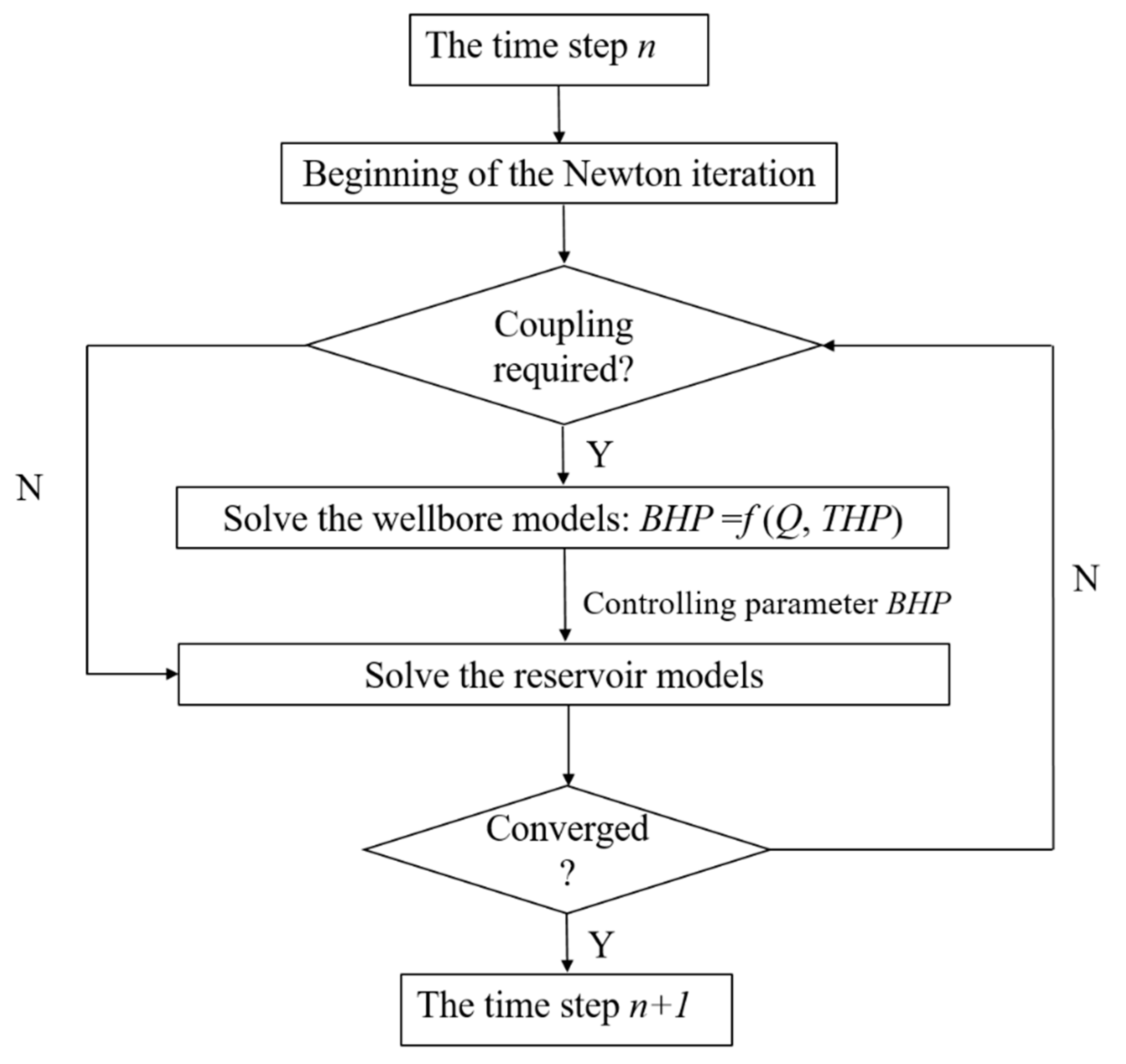
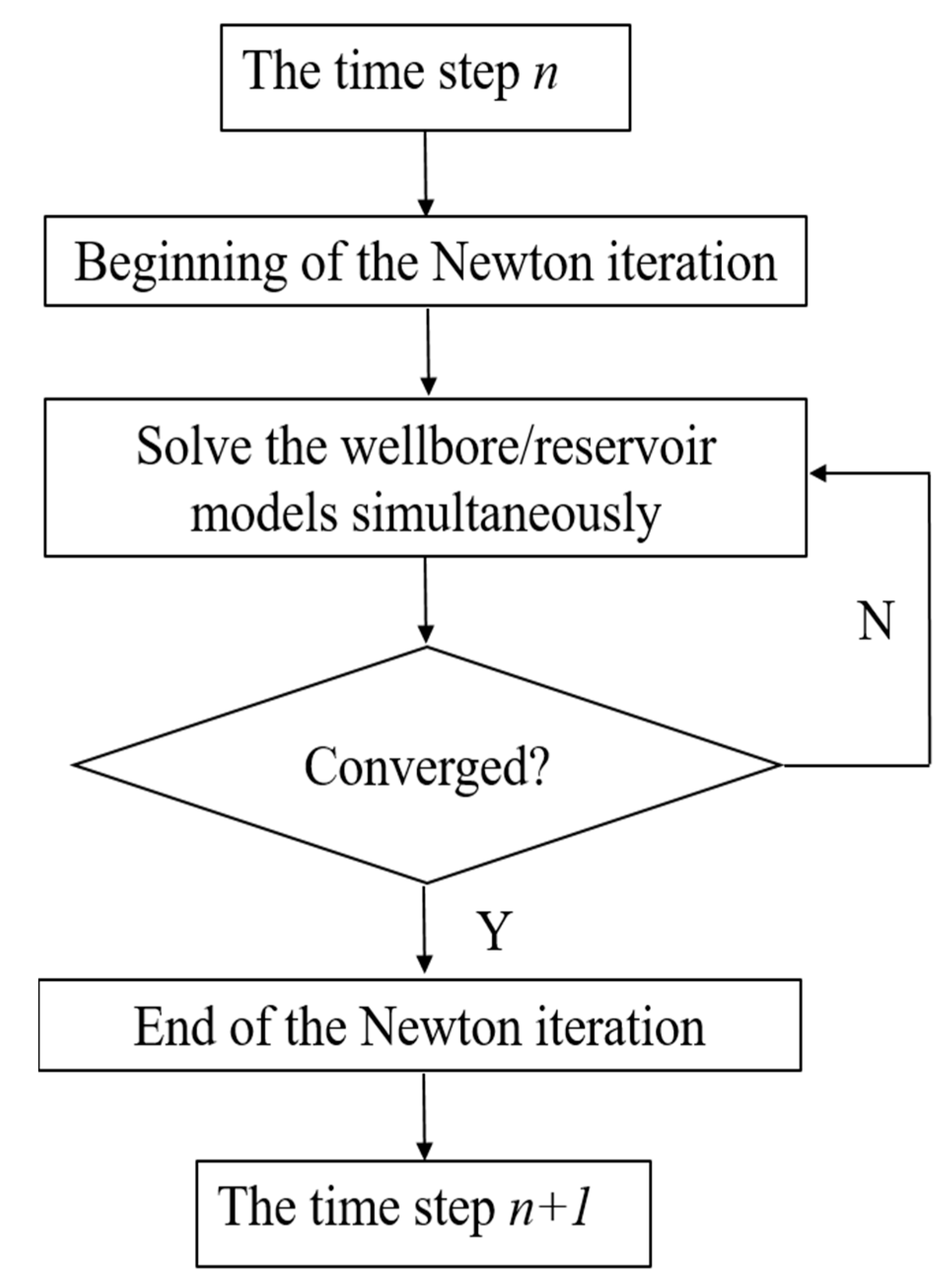
3.3. Numerical Implementation of Coupling Reservoir and Wellbore Models

Numerically implementing the reservoir and wellbore models requires the coupling of two sets of PDEs. The reservoir’s PDEs and wellbore’s PDEs are coupled through source and sink terms in mass balance equations. Meanwhile, the reservoir pressure at the reservoir/wellbore surface must match the wellbore segment pressure. The reservoir models and wellbore models are concurrently solved at each time step. Important control parameters (e.g., phase flow rate, tubing head, and bottom hole pressure) are transferred between these two sets of PDEs. The primary reservoir variables include the moles of hydrocarbon components and water, pressure, temperature, and saturation. The primary wellbore variables contain the moles of hydrocarbon components and water, pressure, temperature, volumetric holdup, and mixture velocity. Once the primary variables in the reservoir and wellbore are resolved, the other variables are updated in the whole coupled systems.

There are three different types of coupling schemes used in a couped reservoir/wellbore simulation: explicit, implicit, and fully implicit [15,26,40,96].

In an explicit coupling scheme, a reservoir and a wellbore are treated as different domains and resolved at different time steps [129,130]. The explicit coupling scheme balances the wellbore and reservoir at the same time step level. This scheme produces less computational burden and is highly flexible for a coupled system. A case in point is an explicit calculation of bottom hole pressure (BHP) as a controlling parameter. Wellbore models calculate the BHP at a specific time step n for a phase rate Q given by the reservoir model and THP. Then one uses the BHP as a well boundary datum to solve reservoir models to obtain a new phase rate Q_new. This new phase rate Q_new is then selected as a new input for wellbore simulation at the next synchronization time step n + 1. Figure 4 summarizes the schematic of the explicit coupling scheme discussed above.

In an implicit coupling scheme, a reservoir and a wellbore are also treated as different domains but balanced at a Newton iteration level. This scheme demands more computational effort than the previous explicit coupling scheme due to the iterative calculation associated with the time step level [129,131]. In the implicit case, a requirement for coupling actions must be determined at the beginning of each Newton iteration. The controlling parameter BHP calculated by wellbore models passes to the reservoir models as a boundary constraint. In the same time step, one uses this converged BHP to solve reservoir models and check the convergence of the reservoir equations. If they converge, one proceeds to the next time step. If they diverge, the iterations are repeated to update Q and THP to calculate the reservoir model and wellbore model until the Newton solution of coupled processes converges. The schematic of the implicit coupling scheme is shown in Figure 5.

In a fully implicit coupling scheme, a reservoir and a wellbore are treated as one domain. Reservoir models and wellbore models are solved simultaneously at each Newton iteration level [129,132]. The Jacobian matrix in the fully implicit scheme is significantly larger than that for independent wellbore or reservoir simulators. The fully implicit coupling scheme needs the most computational effort and produces the most stable solution for a coupled reservoir/wellbore simulation among these three schemes. For a fully implicit case, synchronization points need to be defined where information from the reservoir is synchronously passed to the wellbore. The primary variable parameters (i.e., BHP, reservoir pressure, saturation, moles of hydrocarbon component, and holdups) are solved simultaneously. The fully implicit scheme checks whether the Newton iteration is converged or not. If yes, one proceeds to the next time step. Otherwise, one repeats iteration loops until a Newton iteration converges. The schematic of the fully implicit coupling scheme is presented in Figure 6.

In the above discussed three coupling schemes, the explicit coupling method only balances the reservoir model and wellbore model at the beginning of each time step and fails to generate an accurate reservoir state or wellbore state at the end of each time step. The implicit coupling scheme achieves equilibrium between the reservoir model and wellbore model at the Newton iteration level. However, the implicit solution’s correctness relies on the coupling frequency, and the time step convergence is simply based on the reservoir model. The fully implicit scheme is regarded as the most stable and most accurate coupling method due to the reservoir model and wellbore model being solved simultaneously at the Newton iteration level.

We reviewed the most representative examples of coupled reservoir/wellbore simulations in open publications.

Table 3. Overview of the most representative examples of coupled reservoir/wellbore simulators.

Author (s)	Coupled Reservoir/Wellbore Simulation	Coupling Scheme
Stone et al. [26]	M, T, B, SF, H	F
Almehaideb et al. [14]	M, N, B, SF, V	F
Winterfeld [30]	M, N, B, SM, V	F
Holmes et al. [12]	M, ?, B, DF, M	F
Stone et al. [25]	M, T, C, DF, M	I
Coats et al. [9]	M, N, C, ?, M	F
Bhat et al. [16]	S, T, B, ?, H	I
Nennie et al. [1]	M, T, B, SF, M	E
Sagen et al. [23]	M, T, B, ?, M	F
Pourafshary [22]	M, T, C, DF, V	F
Leemhuis et al. [19]	M, T, B, SF, M	E
Livescu et al. [20]	M, T, C, DF, M	F
Livescu et al. [50]	M, T, B, DF, M	F
Semenova et al. [85]	M, T, C, DF, M	F
Twerda et al. [29]	M, T, B, SF, M	F
Bahonar et al. [15]	S, T, B, ?, V	F
Shirdel [52]	S, N, C, ?, H	F
Pan and Oldenburg [21]	M, T, C, DF, V	F
Gao [129]	M, N, B, SM, V&H	I
Forouzanfar et al. [48]	M, T, C, DF, V	F
Cao et al. [17]	M, N, C, ?, M	F
Olivares [99]	M, N, C, SM, V	F
Redick [130]	M, N, B, ?, V	I
Tang et al. [96]	M, N, C, DF, H	F
Galvao et al. [33]	S, T, C, ?, V	E
Galvao et al. [133]	S, T, C, ?, V	E
Basirat et al. [32]	M, T, C, DF, V	F
Battistelli et al. [31]	M, T, C, DF, V	F
Raad et al. [34]	M, T, B, ?, V	E
Liao et al. [35]	M, T, B, ?, H	F

Legend: Coupled reservoir/wellbore simulation: M = multiphase; S = singlephase; T = thermal; N = non-thermal; B = black oil; C = compositional; SF—separated flow; SM—semi empirical model; DF—Drift-Flux; V—vertical well; H—horizontal well; M—multilateral well; ? —unknown. Coupling scheme: F—fully implicit; I—implicit; E—explicit.

summarizes the most relevant aspects of various coupling examples.

4. Applications of Coupled Reservoir/Wellbore Simulators

4.1. Typical Application 1—Gas Coning

Gas coning is a common gas flow phenomenon where the reservoir’s gas–oil contact migrates slowly to the wellbore due to the drawdown of the oil production in the horizontal or deviated wells. The progress of the gas cone is a gradual transitional process. Once the gas–oil contact reaches the wellbore, the gas–liquid mixture in the wellbore abruptly alters with a steep increase in the gas–oil ratio (GOR), resulting in a substantial decrease in bottom hole pressure. The reservoir simulation usually applies the lift curve to simulate gas coning, while varied GOR values result in various bottom hole pressures. The variation in bottom hole pressure can reflect the occurrence of gas coning. However, reservoir simulation lacks effective simulation of the dynamic transient in the wellbore. Single reservoir simulation can hardly describe the gas breakthrough phenomenon due to a constant productivity index applied. A dynamic coupled wellbore-reservoir simulator was developed to simulate gas coning problems by Nennie et al. and Leemhuis et al. [3,4,19]. Figure 7 shows the BHP at different inflow control valves (ICVs) versus time during the gas breakthrough in a horizontal well with multizone completion by the coupled reservoir/wellbore simulator and simulator MoReS. MoRes is a reservoir simulator that can handle non-fractured and fractured reservoirs. It can be drawn from Figure 4 that the simulation points between the coupled reservoir/wellbore simulator and simulator MoReS are slightly different. A smaller BHP in the coupled reservoir/wellbore simulator makes a larger mass flow to the wellbore than the simulator MoRes, which results in the gas breakthrough occurring 15 h earlier in the coupled simulator. Moreover, the pressure development after gas coning between the coupled reservoir/wellbore simulator and the simulator MoRes indicates a significant difference. The pressure derivative performs much steeper after the gas breakthrough than before. This case reveals how a dynamic reservoir/wellbore simulator influences the gas coning phenomenon more accurately than a single reservoir simulator.

4.2. Typical Application 2—Well Storage Effect

Well storage effect is usually referred to as the well dynamics during start-up and shut-in. Both start-up and shut-in imply a strong interaction between the wellbore and the reservoir. During the well testing, the pressure measurements are collected within the wellbore instead of the reservoir. The pressure recorder is employed to measure the reservoir responses; unfortunately, the wellbore responses are also gathered. Moreover, the wellbore responses are much faster than the reservoir responses. Consequently, the wellbore storage effect between the wellbore and reservoir must be considered during well testing. The researchers from Integrated System Approach Petroleum Production (ISAPP) simulated the dynamic well storage phenomenon to reveal the necessity of a coupled reservoir/wellbore simulator [1,4]. They stated that the coupled reservoir/wellbore model was a Matlab coupling between a single reservoir simulator MoRes and a single wellbore simulator OLGA. Figure 8 presents the BHP versus time for simulations during shut-in and start-up periods from the coupled simulator and OLGA. OLGA is a multi-phase flow simulator that can simulate transient flow behavior in the wellbore. According to Figure 8a, the BHP simulated by OLGA soon reached the original reservoir pressure within several minutes, while the coupled simulator reached the reservoir pressure after six hours during the build-up period after the shut-in operation. Moreover, the reservoir pressure of the coupled simulator was smaller than the initial reservoir pressure due to reservoir depletion. The wellbore storage effect also influences the start-up period, referred to in Figure 8b. The OLGA simulator can simulate the well storage but overrate the BHP due to the missing reservoir depletion. Therefore, the interactions between wellbore and reservoir should be taken into consideration for dynamic procedures such as shut-in, start-up, depletion, and cleanup.

4.3. Typical Application 3—Liquid Loading

Liquid loading is a serious issue when the gas rate fails to lift all the liquids to the surface in most mature gas fields. An accumulation of unproduced liquid in a wellbore causes sudden decreases in gas production and drastic fluctuations in wellbore pressure [134]. Liquid loading can hardly be comprehensively simulated by a reservoir simulator or wellbore simulator due to the flow transience between reservoir and wellbore. Tang et al. [96] developed a fully implicitly coupled reservoir/wellbore simulator to describe the liquid loading phenomenon in horizontal wells. Figure 9 compares the gas-producing rate and the pressure of a perforated well segment from Tang et al.’s coupled simulator and Eclipse 300 (E300). A relevant DF model used in E300 was detailed by Shi et al. [60]. The simulation results revealed a sharp drop in the gas rate and a steep increase in the pressure at the perforated segment at approximately the 60th day. Tang et al.’s simulator forecasted the onset of the liquid loading phenomenon around one day earlier than E300.

4.4. Typical Application 4—General Scenarios

A coupled reservoir/wellbore simulator containing black oil and compositional models proposed by Livescu et al. [20,50] was used in some complex cases. Their case studies revealed various applications for simulating three-phase steady-state flow, gas condensate, thermal flow, phase changes, and compositional fluctuations. Various wellbore types, including vertical wells, horizontal wells, and multilateral wells, are connected to the reservoir by different completion methods. As illustrated in Figure 10, the whole wellbore is split into multiple segments coupling the reservoir girds. The variable parameters in the coupled reservoir/wellbore systems include pressure, temperature, mole fractions, and in situ phase fractions. All these variable parameters are captured at different time steps to accurately describe physical phenomena both in a wellbore and a reservoir. The underlying models are flexible in solving advanced completions and complex downhole networks. Livescu et al.’s coupled simulator was proven with broad applicability and robustness.

5. Summary

In this study, we conducted a literature assessment of the dynamic interactions between wellbores and reservoirs. We explained the wide application of the DF model in the wellbore model for coupling the reservoir models. We honored the fully implicit method for coupling the reservoir system and wellbore system due to its high stability and accuracy. It should be emphasized that dynamic coupled reservoir/wellbore simulators are necessary for resolving transient flow problems between reservoir and wellbore.

Livescu et al. [20,50]; Pourafshary [22]; Cao et al., [17]; Shirdel [52] developed their own coupled reservoir/reservoir models for general scenarios of different wellbore types with advanced completions. The findings of the numerical analysis of pressure, temperature, mole fractions, and in situ phase fractions matched well with experimental data or analytical solutions.

In horizontal or deviated wells, the gas coning phenomenon reflected typical dynamic interactions between reservoir and wellbore. Belfroid et al. [3]; Leemhuis et al. [19]; and Nennie et al. [4], noticed a lower bottom hole pressure and an earlier simulated gas breakthrough time in their dynamically coupled simulator, which performed slightly different simulation results from a standalone reservoir simulator.

During start-up and shut-down, the well exhibited robust dynamics. Alberts et al. [1] and Nennie et al. [4], showed that the bottom hole pressure reached the reservoir pressure more slowly and was smaller than the initial reservoir pressure in the coupled model during the shut-in period. Forouzanfar et al. [48] captured the clear wellbore storage effect by demonstrating an unstable constant pressure derivative value during the radial flow in the drawdown test. Bahonar et al. [15] reported that the coupled model performed better than the commercial well testing simulator in terms of temperature impact and wellbore storage effect.

Tang et al [96], accurately anticipated the gas rate production and pressure of the perforated segment during the liquid loading period. Their coupled model observed the concise flow-pattern transition and forecasted the onset of the liquid loading one day earlier than E300.

More coupled simulators will be utilized to address other transient flow phenomena to further define the necessity of coupling reservoir/wellbore modeling.

References

1. Alberts, G.; Belfroid, S.; Peters, L.; Joosten, G.J. An Investigation into the Need of a Dynamic COUPLED well-Reservoir Simulator. In Proceedings of the SPE Annual Technical Conference and Exhibition, Anaheim, CA, USA, 11–14 November 2007. [Google Scholar] [CrossRef]
2. da Silva, D.; Jansen, J. A Review of Coupled Dynamic Well-Reservoir Simulation. IFAC-PapersOnLine 2015, 48, 236–241. [Google Scholar] [CrossRef]
3. Belfroid, S.; Sturm, W.; Alberts, G.; Peters, R.; Schiferli, W. Prediction of well performance instability in thin layered reservoirs. In Proceedings of the SPE Annual Technical Conference and Exhibition, Dallas, TX, USA, 9–12 October 2005. [Google Scholar] [CrossRef]
4. Nennie, E.D.; Alberts, G.J.N.; Peters, L.; van Donkelaar, E. Using a Dynamic Coupled Well-Reservoir Simulator to Optimize Production of a Horizontal Well in a Thin Oil Rim. In Proceedings of the Abu Dhabi International Petroleum Exhibition and Conference, Abu Dhabi, UAE, 3–6 November 2008. [Google Scholar] [CrossRef]
5. Hasan, A.R.; Kabir, C.S.; Wang, X. Development and Application of a Wellbore/Reservoir Simulator for Testing Oil Wells. SPE Form. Evaluation 1997, 12, 182–188. [Google Scholar] [CrossRef]
6. Hasan, A.R.; Kabir, C.S.; Wang, X. Wellbore Two-Phase Flow and Heat Transfer During Transient Testing. SPE J. 1998, 3, 174–180. [Google Scholar] [CrossRef]
7. Izgec, B.; Kabir, C.S.; Zhu, D.; Hasan, A.R. Transient Fluid and Heat Flow Modeling in Coupled Wellbore/Reservoir Systems. In Proceedings of the SPE Annual Technical Conference and Exhibition, San Antonio, TX, USA, 24–27 September 2006. [Google Scholar] [CrossRef]
8. Kabir, C.S.; Hasan, A.R.; Jordan, D.L.; Wang, X. A Wellbore/Reservoir Simulator for Testing Gas Wells in High-Temperature Reservoirs. SPE Form. Evaluation 1996, 11, 128–134. [Google Scholar] [CrossRef]
9. Coats, B.; Fleming, G.; Watts, J.; Rame, M.; Shiralkar, G. A Generalized Wellbore and Surface Facility Model, Fully Coupled to a Reservoir Simulator. In Proceedings of the SPE Annual Technical Conference and Exhibition, Houston, TX, USA, 3–5 February 2003. [Google Scholar] [CrossRef]
10. Kosmala, A.; Aanonsen, S.I.; Gajraj, A.; Biran, V.; Brusdal, K.; Stokkenes, A.; Torrens, R. Coupling of a Surface Network With Reservoir Simulation. In Proceedings of the SPE Reservoir Simulation Symposium, Denver, CO, USA, 5–8 October 2003. [Google Scholar] [CrossRef]
11. Zapata, V.J.; Brummett, W.M.; Osborne, M.E.; Van Nispen, D.J. Advances in Tightly Coupled Reservoir/ Wellbore/Surface-Network Simulation. SPE Reserv. Evaluation Eng. 2001, 4, 114–120. [Google Scholar] [CrossRef]
12. Holmes, J.; Barkve, T.; Lund, O. Application of a Multisegment Well Model to Simulate Flow in Advanced Wells. In Proceedings of the European petroleum conference, The Hague, Netherlands, 20–22 October 1998. [Google Scholar] [CrossRef]
13. Miller, C.W. Wellbore Storage Effects in Geothermal Wells. Soc. Pet. Eng. J. 1980, 20, 555–566. [Google Scholar] [CrossRef]
14. Almehaideb, R.A.; Aziz, K.; Pedrosa, O.J. A Reservoir/Wellbore Model for Multiphase Injection and Pressure Transient Analysis. In Proceedings of the Middle East Oil Show, Bahrain Exhibition Center, Sanabis, Bahrain, 11–14 March 1989. [Google Scholar] [CrossRef]
15. Bahonar, M.; Azaiez, J.; Chen, Z.J. Transient Nonisothermal Fully Coupled Wellbore/Reservoir Model for Gas-Well Testing, Part 1: Modelling. J. Can. Pet. Technol. 2011, 50, 37–50. [Google Scholar] [CrossRef]
16. Bhat, A.; Swenson, D.; Gosavi, S. Coupling the HOLA wellbore simulator with TOUGH2. In Proceedings of the 30th Workshop on Geothermal Reservoir Engineering, Stanford, CA, USA, 31 January–2 February 2005. [Google Scholar]
17. Cao, H.; Samier, P.; Kalunga, H.; Detige, E.; I Obi, E. A Fully Coupled Network Model, Practical Issues and Comprehensive Comparison with Other Integrated Models on Field Cases. In Proceedings of the SPE Annual Technical Conference and Exhibition, Houston, TX, USA, 28–30 September 2015. [Google Scholar] [CrossRef]
18. Holmes, J. Enhancements to the Strongly Coupled, Fully Implicit Well Model: Wellbore Crossflow Modeling and Collective Well Control. In Proceedings of the SPE Reservoir Simulation Symposium, San Francisco, CA, USA, 15–18 November 1983. [Google Scholar] [CrossRef]
19. Leemhuis, A.P.; Nennie, E.D.; Belfroid, S.P.C.; Alberts, G.J.N.; Peters, L.; Joosten, G.J. Gas Coning Control for Smart Wells Using a Dynamic Coupled Well-Reservoir Simulator. In Proceedings of the Intelligent Energy Conference and Exhibition, Amsterdam, The Netherlands, 25–27 February 2008. [Google Scholar] [CrossRef]
20. Livescu, S.; Durlofsky, L.; Aziz, K.; Ginestra, J. A fully-coupled thermal multiphase wellbore flow model for use in reservoir simulation. J. Pet. Sci. Eng. 2010, 71, 138–146. [Google Scholar] [CrossRef]
21. Pan, L.; Oldenburg, C.M. T2Well—an integrated wellbore–reservoir simulator. Comput. Geosci. 2014, 65, 46–55. [Google Scholar] [CrossRef]
22. Pourafshary, P. A Coupled Wellbore/Reservoir Simulator to Model Multiphase Flow and Temperature Distribution. Ph.D. Thesis, The University of Texas, Austin, TX, USA, 2007. [Google Scholar]
23. Sagen, J.; Østenstad, M.; Hu, B.; Henanger, K.E.I.; Lien, S.K.; Xu, Z.-G.; Groland, S.; Sira, T. A Dynamic Model for Simulation of Integrated Reservoir, Well and Pipeline System. In Proceedings of the SPE Annual Technical Conference and Exhibition, Denver, CO, USA, 30 October–2 November 2011. [Google Scholar] [CrossRef]
24. Satti, R.P.; Gilliat, J.; Bale, D.S.; Hillis, P.; Myers, B.; Harper, J. Application of a Transient Near-Wellbore / Reservoir Simulator for Complex Completions Design. In Proceedings of the Offshore Technology Conference Brasil, Rio de Janeiro, Brazil, 29–31 October 2019. [Google Scholar] [CrossRef]
25. Stone, T.W.; Bennett, J.; Law, D.H.S.; Holmes, J.A. Thermal Simulation with Multisegment Wells. SPE Reserv. Evaluation Eng. 2002, 5, 206–218. [Google Scholar] [CrossRef]
26. Stone, T.; Edmunds, N.; Kristoff, B. A Comprehensive Wellbore/Reservoir Simulator. In Proceedings of the SPE Symposium on Reservoir Simulation, Houston, TX, USA, 6–8 February 1989. [Google Scholar] [CrossRef]
27. Sturm, W.; Belfroid, S.; Van Wolfswinkel, O.; Peters, M.; Verhelst, F. Dynamic reservoir well interaction. In Proceedings of the SPE Annual Technical Conference and Exhibition, Houston, TX, USA, 26–29 September 2004. [Google Scholar] [CrossRef]
28. Tang, H.; Hasan, A.R.; Killough, J. Development and Application of a Fully Implicitly Coupled Wellbore/Reservoir Simulator to Characterize the Transient Liquid Loading in Horizontal Gas Wells. SPE J. 2018, 23, 1615–1629. [Google Scholar] [CrossRef]
29. Twerda, A.; Nennie, E.D.; Alberts, G.; Leemhuis, A.P.; Widdershoven, C. To ICD or Not to ICD? A Techno-economic Analysis of Different Control Strategies Applied to a Thin Oil Rim Dield Case. In Proceedings of the SPE Middle East Oil and Gas Show and Conference, Manama, Bahrain, 25–28 September 2011. [Google Scholar] [CrossRef]
30. Winterfeld, P.H. Simulation of Pressure Buildup in a Multiphase Wellbore/Reservoir System. SPE Form. Evaluation 1989, 4, 247–252. [Google Scholar] [CrossRef]
31. Battistelli, A.; Finsterle, S.; Marcolini, M.; Pan, L. Modeling of coupled wellbore-reservoir flow in steam-like supercritical geothermal systems. Geothermics 2020, 86, 101793. [Google Scholar] [CrossRef]
32. Basirat, F.; Yang, Z.; Bensabat, J.; Levchenko, S.; Pan, L.; Niemi, A. Characterization of CO2 self-release during Heletz Residual Trapping Experiment I (RTE I) using a coupled wellbore-reservoir simulator. Int. J. Greenh. Gas Control 2020, 102, 103162. [Google Scholar] [CrossRef]
33. Galvao, M.S.; Carvalho, M.S.; Barreto, A.B. A coupled transient wellbore/reservoir-temperature analytical mode. SPE J. 2020, 24, 2335–2361. [Google Scholar] [CrossRef]
34. Raad, S.M.J.; Lawton, D.; Maidment, G.; Hassanzadeh, H. Transient non-isothermal coupled wellbore-reservoir modeling of CO2 injection—Application to CO2 injection tests at the CaMI FRS site, Alberta, Canada. Int. J. Greenh. Gas Control. 2021, 111, 103462. [Google Scholar] [CrossRef]
35. Liao, Y.; Wang, Z.; Chao, M.; Sun, X.; Wang, J.; Zhou, B.; Sun, B. Coupled wellbore–reservoir heat and mass transfer model for horizontal drilling through hydrate reservoir and application in wellbore stability analysis. J. Nat. Gas Sci. Eng. 2021, 95, 104216. [Google Scholar] [CrossRef]
36. Hasan, A.R.; Kabir, C.S.; Sarica, C. Fluid Flow and Heat Transfer in Wellbores; Society of Petroleum Engineers: Richardson, TX, USA, 2002. [Google Scholar]
37. Shoham, O. Mechanistic Modeling of Gas-Liquid Two-Phase Flow in Pipes; SPE: Richardson, TX, USA, 2006. [Google Scholar] [CrossRef]
38. Aziz, K. Petroleum Reservoir Simulation; Applied Science Publishers: London, UK, 1979; p. 476. [Google Scholar]
39. Chen, Z. Reservoir Simulation: Mathematical Techniques in Oil Recovery; Society for Industrial and Applied Mathematics: Philadelphia, PA, USA, 2007. [Google Scholar]
40. Iemcholvilert, S. A Research on Production Optimization of Coupled Surface and Subsurface Model. Master’s Thesis, Texas A&M University, College Station, TX, USA, 2013. [Google Scholar]
41. Chen, Z.; Huan, G.; Ma, Y. Computational Methods for Multiphase Flows in Porous Media; Society for Industrial and Applied Mathematics: Philadelphia, PA, USA, 2006. [Google Scholar] [CrossRef]
42. Beggs, D.H.; Brill, J.P. A Study of Two-Phase Flow in Inclined Pipes. J. Pet. Technol. 1973, 25, 607–617. [Google Scholar] [CrossRef]
43. Hagedorn, A.R.; Brown, K.E. Experimental Study of Pressure Gradients Occurring During Continuous Two-Phase Flow in Small-Diameter Vertical Conduits. J. Pet. Technol. 1965, 17, 475–484. [Google Scholar] [CrossRef]
44. Moissis, R.; Griffith, P. Entrance effects in a two-phase slug flow. J. Heat Transfer 1962, 84, 366–370. [Google Scholar] [CrossRef]
45. Orkiszewski, J. Predicting Two-Phase Pressure Drops in Vertical Pipe. J. Pet. Technol. 1967, 19, 829–838. [Google Scholar] [CrossRef]
46. Ros, N. Simultaneous Flow of Gas and Liquid as Encountered in Well Tubing. J. Pet. Technol. 1961, 13, 1037–1049. [Google Scholar] [CrossRef]
47. Holmes, J. Description of the Drift Flux Model in the LOCA Codes RELAPUK. In Proceedings of the Heat and Fluid Flow in Water Reactor Safety, Manchester, UK, 13–15 September 1977. [Google Scholar]
48. Forouzanfar, F.; Pires, A.; Reynolds, A.C. Formulation of a Transient Multi-Phase Thermal Compositional Wellbore Model and its Coupling with a Thermal Compositional Reservoir Simulator. In Proceedings of the SPE Annual Technical Conference and Exhibition, Houston, TX, USA, 28–30 September 2015. [Google Scholar] [CrossRef]
49. Livescu, S.; Durlofsky, L.J.; Aziz, K. A Semianalytical Thermal Multiphase Wellbore-Flow Model for Use in Reservoir Simulation. SPE J. 2010, 15, 794–804. [Google Scholar] [CrossRef]
50. Livescu, S.; Durlofsky, L.J.; Aziz, K.; Ginestra, J.-C. Application of a New Fully-Coupled Thermal Multiphase Wellbore Flow Model. In Proceedings of the SPE Symposium on Improved Oil Recovery, Tulsa, Oklahoma, USA, 20–23 April 2008. [Google Scholar] [CrossRef]
51. Pan, L.; Freifeld, B.; Doughty, C.; Zakem, S.; Sheu, M.; Cutright, B.; Terrall, T. Fully coupled wellbore-reservoir modeling of geothermal heat extraction using CO 2 as the working fluid. Geothermics 2015, 53, 100–113. [Google Scholar] [CrossRef]
52. Shirdel, M. Development of a coupled wellbore-reservoir compositional simulator for damage prediction and remediation. Ph. D thesis, Texas A&M University, College Station, TX, USA, 2013. [Google Scholar]
53. Tang, H.; Hasan, A.R.; Killough, J. A Fully-Coupled Wellbore-Reservoir Model for Transient Liquid Loading in Horizontal Gas Wells. In Proceedings of the SPE Annual Technical Conference and Exhibition, San Antonio, TX, USA, 9–11 October 2017. [Google Scholar] [CrossRef]
54. Woldesemayat, M.A.; Ghajar, A.J. Comparison of void fraction correlations for different flow patterns in horizontal and upward inclined pipes. Int. J. Multiph. Flow 2007, 33, 347–370. [Google Scholar] [CrossRef]
55. Ishii, M.; Mishima, K. Two-fluid model and hydrodynamic constitutive relations. Nucl. Eng. Des. 1984, 82, 107–126. [Google Scholar] [CrossRef]
56. Bonizzi, M.; Issa, R. On the simulation of three-phase slug flow in nearly horizontal pipes using the multi-fluid model. Int. J. Multiph. Flow 2003, 29, 1719–1747. [Google Scholar] [CrossRef]
57. Hibiki, T.; Takamasa, T.; Ishii, M. One-Dimensional Drift-Flux Model and Constitutive Equations for Relative Motion Between Phases in Various Two-Phase Flow Regimes at Microgravity Conditions. In Proceedings of the International Conference on Nuclear Engineering, Arlington, VA, USA, 25–29 April 2004; pp. 377–386. [Google Scholar] [CrossRef]
58. Hoeld, A. Coolant channel module CCM: An universally applicable thermal-hydraulic drift-flux based mixture-fluid 1D model and code. Nucl. Eng. Des. 2007, 237, 1952–1967. [Google Scholar] [CrossRef]
59. Zuber, N.; Findlay, J.A. Average Volumetric Concentration in Two-Phase Flow Systems. J. Heat Transf. 1965, 87, 453–468. [Google Scholar] [CrossRef]
60. Shi, H.; Holmes, J.; Diaz, L.R.; Durlofsky, L.J.; Aziz, K. Drift-Flux Parameters for Three-Phase Steady-State Flow in Wellbores. SPE J. 2005, 10, 130–137. [Google Scholar] [CrossRef]
61. Shi, H.; Holmes, J.A.; Durlofsky, L.J.; Aziz, K.; Diaz, L.R.; Alkaya, B.; Oddie, G. Drift-Flux Modeling of Two-Phase Flow in Wellbores. SPE J. 2005, 10, 24–33. [Google Scholar] [CrossRef]
62. Jepson, W.; Taylor, R. Slug flow and its transitions in large-diameter horizontal pipes. Int. J. Multiph. Flow 1993, 19, 411–420. [Google Scholar] [CrossRef]
63. Coddington, P.; Macian, R. A study of the performance of void fraction correlations used in the context of drift-flux two-phase flow models. Nucl. Eng. Des. 2002, 215, 199–216. [Google Scholar] [CrossRef]
64. Bestion, D. The physical closure laws in the CATHARE code. Nucl. Eng. Des. 1990, 124, 229–245. [Google Scholar] [CrossRef]
65. Chexal, B.; Lellouche, G.; Horowitz, J.; Healzer, J. A void fraction correlation for generalized applications. Prog. Nucl. Energy 1992, 27, 255–295. [Google Scholar] [CrossRef]
66. Gardner, G. Fractional vapour content of a liquid pool through which vapour is bubbled. Int. J. Multiph. Flow 1980, 6, 399–410. [Google Scholar] [CrossRef]
67. Inoue, A.; Kurosu, T.; Yagi, M.; Morooka, S.; Hoshide, A.; Ishizuka, T.; Yoshimura, K. In-Bundle Void Measurement of a BWR Fuel Assembly by an X-ray CT Scanner: Assessment of BWR Design Void Correlation and Development of New Void Correlation. In Proceedings of the 2nd ASME-JSME International Conference on Nuclear Engineering, San Francisco, CA, USA, 21–23 March 1993. [Google Scholar]
68. Hibiki, T.; Ishii, M. One-Dimensional Drift-Flux Model and Constitutive Equations for Relative Motion between Phases in Various Two-Phase Flow Regimes; Argonne National Lab: Lemont, IL, USA, 1977. [Google Scholar]
69. Liao, L.; Parlos, A.; Griffith, P. Heat Transfer, Carryover and Fall Back in PWR Steam Generators during Transients; MIT Press: Cambridge, MA, USA, 1985. [Google Scholar]
70. Maier, D.; Coddington, P. Validation of RETRAN-03 against a wide range of rod bundle void fraction data. Trans. Am. Nucl. Soc. 1996, 75, 372–374. [Google Scholar]
71. Pearson, K.; Cooper, C.; Jowitt, D. The THETIS 80% Blocked Cluster Experiment. Part 4: Gravity Reflood Experiments; INIS: Winfrith, UK, 1984. [Google Scholar]
72. Sonnenburg, H. Full-Range Drift-Flux Model based on the Combination of Drift-Flux Theory with Envelope Theory. In Proceedings of the Fourth International Topical Meeting on Nuclear Reactor Thermal-Hydraulics (NURETH-4), Karlsruhe, Germany, 10–13 October 1989. [Google Scholar]
73. Sun, K.; Duffey, R.; Peng, C. A Thermal-Hydraulic Analysis of Core Uncovery. In Proceedings of the 19th National Heat Transfer Conference, Experimental and Analytical Modeling of LWR Safety Experiments, Orlando, FL, USA, 27–30 July 1980; pp. 1–10. [Google Scholar]
74. Takeuchi, K.; Young, M.Y.; Hochreiter, L.E. Generalized Drift Flux Correlation for Vertical Flow. Nucl. Sci. Eng. 1992, 112, 170–180. [Google Scholar] [CrossRef]
75. Hasan, A.R.; Kabir, C.S. A Simplified Model for Oil/Water Flow in Vertical and Deviated Wellbores. SPE Prod. Facil. 1999, 14, 56–62. [Google Scholar] [CrossRef]
76. Hasan, A.R.; Kabir, C.S. Predicting Multiphase Flow Behavior in a Deviated Well. SPE Prod. Eng. 1988, 3, 474–482. [Google Scholar] [CrossRef]
77. Hasan, A.R.; Kabir, C.S. A Study of Multiphase Flow Behavior in Vertical Wells. SPE Prod. Eng. 1988, 3, 263–272. [Google Scholar] [CrossRef]
78. Ansari, A.; Sylvester, N.; Shoham, O.; Brill, J. A comprehensive mechanistic model for upward two-phase flow in wellbores. SPE Prod. Facil. 1994, 9, 143–151. [Google Scholar] [CrossRef]
79. Flores, J.G.; Sarica, C.; Chen, T.X.; Brill, J.P. Investigation of Holdup and Pressure Drop Behavior for Oil-Water Flow in Vertical and Deviated Wells. J. Energy Resour. Technol. 1998, 120, 8–14. [Google Scholar] [CrossRef]
80. Hasan, A.; Kabir, C.; Sayarpour, M. Simplified two-phase flow modeling in wellbores. J. Pet. Sci. Eng. 2010, 72, 42–49. [Google Scholar] [CrossRef]
81. Petalas, N.; Aziz, K. A Mechanistic Model for Multiphase Flow in Pipes. J. Can. Pet. Technol. 2000, 39. [Google Scholar] [CrossRef]
82. Tang, H.; Bailey, W.; Stone, T.; Killough, J. A Unified Gas-Liquid Drift-Flux Model for Coupled Wellbore-Reservoir Simulation. In Proceedings of the SPE Annual Technical Conference and Exhibition, Calgary, AB, Canada, 30 September–2 October 2019. [Google Scholar] [CrossRef]
83. Tang, H.; Bailey, W.J.; Stone, T.; Killough, J. A Unified Gas/Liquid Drift-Flux Model for All Wellbore Inclinations. SPE J. 2019, 24, 2911–2928. [Google Scholar] [CrossRef]
84. Oddie, G.; Shi, H.; Durlofsky, L.; Aziz, K.; Pfeffer, B.; Holmes, J. Experimental study of two and three phase flows in large diameter inclined pipes. Int. J. Multiph. Flow 2003, 29, 527–558. [Google Scholar] [CrossRef]
85. Semenova, A.; Livescu, S.; Durlofsky, L.J.; Aziz, K. Modeling of multisegmented thermal wells in reservoir simulation. In Proceedings of the SPE EUROPEC/EAGE Annual Conference and Exhibition, Barcelona, Spain, 14–17 June 2010. [Google Scholar] [CrossRef]
86. Cao, H. Development of Techniques for General Purpose Simulators. Ph.D. Thesis, Stanford University, Stanford, CA, USA, 2002. [Google Scholar]
87. Jiang, Y. A Flexible Computational Framework for Efficient Integrated Simulation of Advanced Wells and Unstructured Reservoir Models. Ph.D. Thesis, Stanford University, Stanford, CA, USA, 2007. [Google Scholar]
88. Schlumberger. Eclipse Technical Description; Schlumberger: Houston, TX, USA, 2010. [Google Scholar]
89. Luo, L.; Cheng, S.; Lee, J. Characterization of refracture orientation in poorly propped fractured wells by pressure transient analysis: Model, pitfall, and application. J. Nat. Gas Sci. Eng. 2020, 79, 103332. [Google Scholar] [CrossRef]
90. Piasecka, M.; Strąk, K.; Maciejewska, B. Heat transfer characteristics during flow along horizontal and vertical minichannels. Int. J. Multiph. Flow 2021, 137, 103559. [Google Scholar] [CrossRef]
91. Wu, Y.; Cheng, L.; Huang, S.; Bai, Y.; Jia, P.; Wang, S.; Xu, B.; Chen, L. An approximate semianalytical method for two-phase flow analysis of liquid-rich shale gas and tight light-oil wells. J. Pet. Sci. Eng. 2019, 176, 562–572. [Google Scholar] [CrossRef]
92. Choi, J.; Pereyra, E.; Sarica, C.; Park, C.; Kang, J.M. An Efficient Drift-Flux Closure Relationship to Estimate Liquid Holdups of Gas-Liquid Two-Phase Flow in Pipes. Energies 2012, 5, 5294–5306. [Google Scholar] [CrossRef]
93. Bhagwat, S.M.; Ghajar, A.J. A flow pattern independent drift flux model based void fraction correlation for a wide range of gas–liquid two phase flow. Int. J. Multiph. Flow 2014, 59, 186–205. [Google Scholar] [CrossRef]
94. Tang, H.; Sun, Z.; He, Y.; Chai, Z.; Hasan, A.R.; Killough, J. Investigating the pressure characteristics and production performance of liquid-loaded horizontal wells in unconventional gas reservoirs. J. Pet. Sci. Eng. 2019, 176, 456–465. [Google Scholar] [CrossRef]
95. Choi, J. TUFFP Multiphase Flow Database, Fluid Flow Project Database, Version 1.1; University of Tulsa: Tulsa, OK, USA, 2013. [Google Scholar]
96. Tang, H. Development and Applications of a Fully Implicitly Coupled Wellbore-Reservoir Simulator. Ph. D thesis, Texas A&M University, College Station, TX, USA, 2019. [Google Scholar]
97. Yan, B. Development of general unstructured reservoir utility and fractured reservoir modeling. Ph.D. Thesis, Texas A&M University, College Station, TX, USA, 2017. [Google Scholar]
98. Valbuena Olivares, E. Production Performance Modeling through Integration of Reservoir and Production Network with Asphaltene Deposition. Ph.D. Thesis, Texas A&M University, College Station, TX, USA, 2015. [Google Scholar]
99. Eaton, B. The Prediction of Flow Patterns, Liquid Holdup and Pressure Losses Occurring During Continuous Two-Phase Flow in Horizontal Pipes. Ph. D. Thesis, University of Tulsa, College Station, OK, USA, 1965. [Google Scholar]
100. Beggs, H.D. An Experimental Study of Two-Phase Flow in Inclined Pipes. Ph. D. Thesis, University of Tulsa, College Station, OK, USA, 1973. [Google Scholar]
101. Schmidt, Z. Experimental Study of Gas-Liquid Flow in a Pipeline-Riser Pipe System. Master’s Thesis, University of Tulsa, College Station, OK, USA, 1976. [Google Scholar]
102. Cheremisinoff, N.P. Experimental and Theoretical Investigation of Horizontal Stratified and Annular Two-Phase Flow with Heat Transfer. Ph. D. Thesis, Clarkson University, College Station, NY, USA, 1977. [Google Scholar]
103. Mukherjee, H. An Experimental Study of Inclined Two-Phase Flow. Ph. D. Thesis, University of Tulsa, College Station, OK, USA, 1980. [Google Scholar]
104. Akpan, I.B. Two-Phase Metering. Master’s Thesis, University of Tulsa, College Station, OK, USA, 1980. [Google Scholar]
105. Vongvuthipornchai, S. Experimental Study of Pressure Wave Propagation in Two-Phase Mixtures. Ph. D. Thesis, University of Tulsa, College Station, OK, USA, 1980. [Google Scholar]
106. Minami, K.L. Liquid Holdup in Wet-Gas Pipelines. Master’s Thesis, University of Tulsa, College Station, OK, USA, 1983. [Google Scholar]
107. Caetano, E.F. Upward Vertical Two-Phase Flow Through an Annulus. Ph. D. Thesis, University of Tulsa, College Station, OK, USA, 1986. [Google Scholar]
108. Kouba, G. Horizontal Slug Flow Modeling and Metering. Ph. D. Thesis, University of Tulsa, College Station, OK, USA, 1986. [Google Scholar]
109. Rothe, P.H.; Crowley, C.J.; Sam, R.G. Investigation of Two-Phase Flow in Horizontal Pipes at Large Pipe Size and High Gas Density. Technical Report, American Gas Association Pipeline Research Committee Project, PR 172-507. Available online: https://www.genuinepdfs.com/product/PRCI-PR172-507/ (accessed on 23 June 2022).
110. Felizola, H. Slug Flow in Extended Reach Directional Wells. Master’s Thesis, University of Tulsa, College Station, OK, USA, 1992. [Google Scholar]
111. Roumazeilles, P. An Experimental Study of Downward Slug Flow in Inclined Pipes. Master’s Thesis, University of Tulsa, College Station, OK, USA, 1994. [Google Scholar]
112. Brill, J.P.; Chen, X.T.; Flores, J.G.; Marcano, R. Transportation of Liquids in Multiphase Pipelines under Low Liquid Loading Conditions; Final Report, University of Tulsa Fluid Flow Project; University of Tulsa: Tulsa, OK, USA, 1996. [Google Scholar]
113. Meng, W. Low Liquid Loading Gas-Liquid Two-Phase Flow in Near-Horizontal Pipes. Ph. D. Thesis, University of Tulsa, College Station, OK, USA, 1999. [Google Scholar]
114. Abdul-Majeed, G.H. Liquid Slug Holdup in Horizontal and Slightly Inclined Two-Phase Slug Flow. J. Pet. Sci. Eng. 2000, 27, 27–32. [Google Scholar] [CrossRef]
115. Fan, Y. An Investigation of Low Liquid Loading Gas-Liquid Stratified Flow in Near-Horizontal Pipes. Ph. D. Thesis, University of Tulsa, College Station, OK, USA, 2005. [Google Scholar]
116. John, G.W. A Study of Gas-Liquid Pipe Flow. Ph. D. Thesis, University of Tulsa, College Station, OK, USA, 2005. [Google Scholar]
117. Magrini, K.L. Liquid Entrainment in Annular Gas-Liquid Flow in Inclined Pipes. Master’s Thesis, University of Tulsa, College Station, OK, USA, 2009. [Google Scholar]
118. Yuan, G. Liquid Loading of Gas Wells. Master’s Thesis, University of Tulsa, College Station, OK, USA, 2011. [Google Scholar]
119. Guner, M. Liquid Loading of Gas Wells with Deviations from 0 to 45. Ph. D. Thesis, University of Tulsa, College Station, OK, USA, 2012. [Google Scholar]
120. Alsaadi, Y. Liquid Loading in Highly Deviated Gas Wells. Ph. D. Thesis, University of Tulsa, College Station, OK, USA, 2013. [Google Scholar]
121. Li, Y.; Bailey, W.; Rashid, K.; Couët, B.; Shippen, M.; Holmes, J. Optimized Parameters and Extension of a 2-Phase Flow-Regime-Independent FLOW model. In Proceedings of the 15th International Conference on Multiphase Production Technology, Cannes, France, 15–17 June 2011. [Google Scholar]
122. Ishii, M.; Hibiki, T. Thermo-Fluid Dynamics of Two-Phase Flow; Springer Science & Business Media: Berlin/Heidelberg, Germany, 2010. [Google Scholar]
123. Govier, G.W.; Aziz, K.; Schowalter, W.R. The Flow of Complex Mixtures in Pipes; Van Nostrand Reinhold Company: New York, NY, USA, 1972. [Google Scholar] [CrossRef]
124. Dong, C.C.; Bahonar, M.; Chen, Z.J.; Azaiez, J. Development of an Algorithm of Dynamic Gridding for Multiphase Flow Calculation in Wells. J. Can. Pet. Technol. 2011, 50, 35–44. [Google Scholar] [CrossRef]
125. Ramey, H.J. Wellbore Heat Transmission. J. Pet. Technol. 1962, 14, 427–435. [Google Scholar] [CrossRef]
126. Satter, A. Heat Losses During Flow of Steam Down a Wellbore. J. Pet. Technol. 1965, 17, 845–851. [Google Scholar] [CrossRef]
127. Xiong, W.; Bahonar, M.; Chen, Z. Development of a Thermal Wellbore Simulator with Focus on Improving Heat Loss Calculations for SAGD Steam Injection. In Proceedings of the SPE Canada Heavy Oil Technical Conference, Calgary, AB, Canada, 9–11 June 2015. [Google Scholar] [CrossRef]
128. Yoshida, N. Modeling and Interpretation of Downhole Temperature in a Horizontal Well with Multiple Fractures. Ph.D. Thesis, Texas A&M University, College Station, TX, USA, 2016. [Google Scholar]
129. Gao, M. Reservoir and Surface Facilities Coupled through Partially and Fully Implicit Approaches. Master’s Thesis, Texas A&M University, College Station, TX, USA, 2014. [Google Scholar]
130. Redick, B.S. PID Controlled Adaptive Time-Stepping in Coupled Surface-Subsurface Simulation: A Tool for Reducing Non-Physical Oscillation. Master Thesis, Texas A&M University, College Station, TX, USA, 2017. [Google Scholar]
131. Trick, M. A Different Approach to Coupling a Reservoir Simulator with a Surface Facilities Model. In Proceedings of the SPE Gas Technology Symposium, Calgary, AB, Canada, 15–18 March 1998. [Google Scholar] [CrossRef]
132. Ghorayeb, K.; Holmes, J.; Torrens, R.; Grewal, B. A general purpose controller for coupling multiple reservoir simulations and surface facility networks. In Proceedings of the SPE Reservoir Simulation Symposium, Houston, TX, USA, 3–5 February 2003. [Google Scholar] [CrossRef]
133. Galvao, M.S.; Carvalho, M.S.; Barreto, A.B. Thermal impacts on pressure transient tests using a coupled wellbore/reservoir analytical model. J. Pet. Sci. Eng. 2020, 191, 106992. [Google Scholar] [CrossRef]
134. Lea, J.F.; Nickens, H.V. Solving gas-well liquid-loading problems. J. Pet. Technol. 2004, 56, 30–36. [Google Scholar] [CrossRef]
Figure 1. Spatial and time scales for the reservoir (R) and wellbore (W) phenomena. This figure was modified from Figure 1 in ref [4].
Processes 10 01778 g001
Figure 2. Schematic of DF models. This figure was modified from Figure 1 in ref [60].
Processes 10 01778 g002
Figure 3. Three forms of the expression for inclination multiplier m(θ). This figure was modified from ref [60,77,83].
Processes 10 01778 g003
Figure 4. Schematic of the explicit coupling scheme.
Processes 10 01778 g004
Figure 5. Schematic of the implicit coupling scheme.
Processes 10 01778 g005
Figure 6. Schematic of the fully implicit coupling scheme.
Processes 10 01778 g006
Figure 7. BHP at different ICVs versus time during gas breakthrough. This figure was modified from Figure 7 in ref [4].
Processes 10 01778 g007
Figure 8. Comparisons of BHP versus time (a) build-up period after shut-in and (b) start-up period from coupled simulator and OLGA. This figure was modified from Figures 9 and 14 in ref [4].
Processes 10 01778 g008
Figure 9. Comparisons of (a) gas-producing rate and (b) the pressure of a perforated segment from Tang et al.’s coupled reservoir/wellbore simulator and E300. This figure was modified from Figure 4.7 in ref [96].
Processes 10 01778 g009
Figure 10. Schematic representation of multilateral wells: (a) dual-lateral well; (b) multilateral well with three branches. This figure was modified from Figure 2 in ref [20] and Figure 6 in ref [50].
Processes 10 01778 g010