1. Introduction
A heat diffusion equation is a partial differential equation (PDE) that models the spatial distribution and the time evolution of temperature in a body under specific initial and boundary conditions [
1,
2,
3,
4], it is widely used in heat transfer process [
5,
6,
7], and it can be formulated from one to three spatial dimensions and one temporal dimension, in such case it would contain a transient state. It can also be found in rectangular, cylindrical, and spherical coordinates.
The classic way to solve the one-dimensional heat diffusion equation is through the method of separation of variables. In this method, the initial condition is approximated by an infinite number of sinusoidal terms, or more specifically, by a Fourier series. The solution to the heat equation will have as many terms as addends have been employed to approximate the initial condition [
8]; therefore, this method is also referred to as the Fourier method and is used in [
9,
10].
Heat polynomials are polynomials that are solutions to the one-dimensional heat diffusion equation [
11]. They were defined by Laplace in 1810 and studied by Chebyshev in 1859 [
12]. Later in 1684, Hermite wrote about them, so they became known as “Hermite Polynomials” [
13,
14]. Applications of the heat polynomial are diverse, and they are extensively discussed in [
15]. A first example of its use consists in determining the temperatures distribution in a homogeneous rod when one of its ends is subjected to a finite flow of constant surface heat. A second example of its use is the determination of the Biot number [
16], a quantity of significant importance since it provides a relationship between heat transfer by convection and heat transfer by conduction when both are present. Heat polynomials are defined in terms of a spatial variable
x, and a temporary variable
t, so they satisfy the one-dimensional heat diffusion equation [
17,
18,
19].
Several contributions are intended to provide solutions to the heat diffusion equation. For example, in [
20,
21], an analytical solution is proposed to the two-dimensional heat diffusion equation; likewise, in [
22,
23,
24], analytical and numerical solutions to the three-dimensional heat equation are presented. Additionally, in [
25], an analytical solution is provided to equation that governs heat transfer in a cooling process. In [
26,
27], analytical and semi-analytical solutions, respectively, are presented to solve heat transfer problems on irregular or anisotropic media. Unlike previous works, in [
28], the authors go further and provide a general method to finding closed solutions to the heat diffusion equation.
Heat conduction problems are the main application that makes use of the heat diffusion equation. The solution strategies provided in this work are aimed at solving these types of problems, thus, some related works will be indicated. In [
29,
30], a problem consisting of identifying a heat source is solved. In [
31], non-local time models are used to describe small-scale thermal processes, which incorporate heat flow memory. These models are transformed to simpler ones that are no more complicated to solve than the classical heat equation. In [
32], the heat conduction problem is solved numerically for the new proposed functionally graded porosity media. In [
33], the inverse heat conduction problem is solved using Trefftz functions that satisfy the heat diffusion equation, but they are characterized by their lack of analytical form. Finally, in [
34], a method to find heat conduction models by machine learning is developed. The learned PDEs are solved by conventional numerical methods. In diffusive convective heat transfer processes in porous media [
35,
36], it is also common to find the heat diffusion equation.
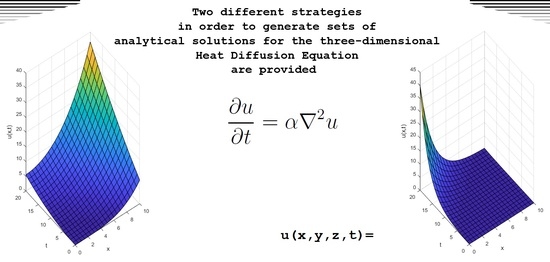
The main objective of this article is to provide two different strategies to generate closed solutions to the three-dimensional heat diffusion equation with transient state and without heat generation. These strategies consist of formulas that generate scalar fields of two different types, polynomial and exponential, which satisfy the heat diffusion equation in three dimensions analytically. At the end of the study, it is concluded that each strategy, in effect, generates an infinite number of solutions to the three-dimensional heat diffusion equation. In addition, two findings are made, the first one is an intrinsic relationship between the coefficients of the one-dimensional polynomials and the coefficients of three-dimensional polynomials, and the second one is a relation between the polynomial solution and the exponential solution. The application of the obtained results is shown by using a heat polynomial to describe a heat conduction phenomenon. Through Remark 1, one-dimensional heat diffusion equation is introduced.
Remark 1. The one-dimensional heat diffusion Equation (1) is obtained from Fourier’s law and the principle of conservation of energy.where with is a scalar field that represents the temperature distribution in the body of study and constitutes the unknown function in the heat diffusion equation; both x and t are the independent variables, x represents the spatial variable, while t represents the temporal variable. Literal α is the thermal diffusivity measured in ms and it is calculated as , where is the thermal conductivity measured in Wm·K, ρ is the density of the body measured in kgm, and is its thermal capacity measured in Jkg·K. To facilitate the identification of the literals used, in
Table 1 the description of each number of the parameters used throughout the entire text is presented.
As background, the heat polynomial is presented. Typically, a single formula is presented to generate them, but here a slight novelty is introduced. Two formulas that are distinguished by the parity of the exponents for the spatial variable x will be presented. The use of one or the other is left to the user’s choice. The user must only establish the value of the literal , which will be the number of terms in the polynomial. For each formula, a recursive equation of variable parameters is attached, which serves to generate the coefficients of each term in the heat polynomial. Likewise, the initial condition for the recursive equation is provided.
Equation (2) generates polynomials with even exponents for the spatial variable, while Equation (3) generates polynomials with odd exponents for the spatial variable. In both cases, obtaining the coefficients
is performed recursively, as shown.
The recursive equations attached to Equations (2) and (3) were solved, so equations generating the heat polynomials with such built-in solutions are rewritten in Equations (
4) and (
5), respectively.
Note that the linear combination of two or more generated heat polynomials is also a solution to the heat diffusion equation in its one-dimensional form (
1).
2. Materials and Methods
In this section the two strategies for generating analytical solutions to the three-dimensional heat diffusion equation will be presented, but before that, this equation will be introduced through Remark 2.
Remark 2. The equation that describes the propagation of heat in an isotropic and homogeneous medium in three dimensions is presented in Equation (
6).
This equation written in a compact form is presented in Equation (
7).
where , with is a scalar field that represents the temperature distribution in the body of study and it is the unknown function in the heat diffusion equation. Literals x, y, z are the spatial coordinates, and t is the temporary variable, all of them are independent variables. Similar to in Equation (1), parameter α is the thermal diffusivity measured in ms. 2.1. Polynomial Solution Strategy
The formula whose goal is to generate polynomials that are solutions to the three-dimensional heat diffusion equation will be presented, but before that, two simple parameters must be defined by the user.
The parameter N constitutes the number of terms that the polynomial will have for each spatial variable, so this literal can only take values from the set of natural numbers, that is, .
For each N selected, it will be possible to generate two different solutions that will be distinguished by the parity of the exponents of the spatial variables x, y, and z. The parameter that allows choosing one solution or another is q. If , then all the exponents of the spatial variables will be even, while if , then they will be odd.
Another simple additional parameter involved in this strategy is denoted by the literal
p, it depends only on the literal
N, and it is calculated as follows.
In Equation (9), the formula to generate polynomials, which are solutions to the three-dimensional heat diffusion equation, is presented.
Note from Equation (9) that only when does the generated polynomial contain an additional term that is a function of the temporary variable only. Note also that, as for the one-dimensional heat polynomials, a recursive equation is used to generate the coefficients of the spatial variables. The literals , , and , meanwhile, are arbitrary real constants.
The recursive equation attached to Equation (9) has been solved, so this equation is rewritten in Equation (
10).
Two polynomials will then be generated from this formula, one with even exponents and one with odd exponents for the spatial variables. The proofs that both are solutions to the three-dimensional heat equation will be presented.
Let
and
, then
. The generated polynomial is presented in Equation (
11).
It will be verified that the polynomial appearing in Equation (
11) is, indeed, a solution of the three-dimensional heat diffusion equation. Below, the derivatives of this polynomial that were made according to the Equation (
6) are shown.
Substitution of (12) into (
6) yields the expression shown in (
13), whose identity proves that polynomial given in (
11) is a solution to the heat diffusion equation described in (
6).
Let
and
, then
. The generated polynomial is presented in Equation (
14).
It will be verified that the polynomial appearing in Equation (
14) is, indeed, a solution of the three-dimensional heat diffusion equation. Below, the derivatives of this polynomial that were made according to Equation (
6) are shown.
Substitution of (15) into (
6) yields the expression shown in (
16), whose identity proves that polynomial given in (
14) is a solution to the heat diffusion equation described in (
6).
After just having proved that both particular polynomial solutions satisfy to heat diffusion equation in three dimensions, through Remark 3 a classic conclusion in the field of differential equations is highlighted.
Remark 3. The linear combination of two or more polynomials generated from Equation (
10)
is also a solution to three-dimensional heat diffusion equation. 2.2. Exponential Solution Strategy
The closed exponential solution proposed to the three-dimensional heat diffusion equation is the following.
Here, x, y, and z are the spatial variables, while t is the temporal variable; all of them are independent variables. The coefficients , ⋯, are arbitrary real constants.
For the purpose of writing the above equation in a more compact way,
, and
are performed. Then Equation (
17) is rewritten in Equation (
18).
As can be seen from Equation (
17), the coefficient of the literal
t is constituted by the sum of the squares of the arbitrary constants
,
, and
, so this coefficient cannot be negative.
It will be verified that the exponential solution appearing in Equation (
17) is, indeed, a solution of the three-dimensional heat diffusion equation. Below, the derivatives of this expression that were made according to Equation (
6) are shown.
Substitution of (19) into (
6) yields the expression shown in (
20), whose identity proves that the function given in (
17) is a solution to the heat diffusion equation described in (
6).
Remark 4. Both the polynomial and exponential analytical solutions cannot be obtained by the method of separation of variables.
2.3. Validation of the Solutions
To validate the analytical solutions generated with each of the proposed solution strategies, such solutions will be compared with the corresponding numerical solutions of the heat diffusion equation. The method of finite differences is used to obtain the numerical solution to the heat diffusion equation. The discretization of the equation is carried out in its implicit form because it has greater stability than the explicit form, and because it does not have restrictions on the values of the space and time differentials. To make a fair comparison, the numerical solutions are obtained using the initial and boundary conditions present in the analytical solutions.
The discretized one-dimensional heat diffusion equation is shown in Equation (
21). This equation was applied to each of its nodes in the mesh.
where,
i is the iterative index for the spatial variable, and
j is the iterative index for the temporal variable.
Remember that, applying the method of finite differences in its implicit form, a matrix system must be solved for each iteration on the time axis. The size of this matrix system coincides with the number of nodes on the spatial axis.
3. Results
Two strategies to generate closed solutions that satisfy the three-dimensional heat diffusion equation with transient state and without internal heat generation are the main result of this study. These two strategies consist of explicit formulas capable of generating an infinite number of solutions to the three-dimensional heat diffusion equation. The traditional solutions obtained with the method of separation of variables consist of the product of two functions, one that depends only on time and the other one that depends only on space. The solutions generated with the strategies proposed here cannot be obtained by this method because such solutions consist of several terms that are necessary to all them satisfy the heat diffusion equation.
The simplest way to generate the coefficients for each of the terms in the polynomial is through recursive equations. These recursive equations have variable coefficients, which increases their complexity; however, in this text such equations are solved in an explicit manner, which greatly facilitate the generation of the polynomials, especially if they are intended to be programmed since they save computing time.
3.1. Solution Graphs
That partial differential equation (PDE) addressed in this study is multidimensional makes it impossible to draw the graphs of the scalar fields, which are solutions to the heat diffusion equation; however, that terms for each spatial variable in the solutions have the same algebraic structure allows outlining the behavior of temperature graphically using a single spatial variable. In other words, the graphs of the scalar fields of the solutions to the three-dimensional heat diffusion equation will be presented using only the spatial variable x. The behavior of the remaining spatial variables can be understood as similar.
The scalar fields that are solutions of the heat diffusion equation were plotted using the R2017b version of Matlab® Natick, MA, USA. These graphs are presented and analyzed below. The domain of the analytic solutions is the entire space; however, to view the graphs, it was decided to use the interval for the spatial variable, and the interval for the temporal variable.
It can be verified that the scalar field corresponding to the polynomial given in Equation (
11) presents a typical behavior of a function whose spatial variable contains even exponents (
Figure 1). This means that the temperature increases with the spatial variable on both the positive and negative axes. Since
, the temperature increases positively, while if
, the temperature would increase negatively. In addition, it can be seen that the temperature increases with time on the positive side of the space axis.
It can be verified that the scalar field corresponding to the polynomial given in Equation (
14) presents a typical behavior of a function whose spatial variable contains odd exponents (
Figure 2). This means that the temperature increases with the spatial variable on the positive axis and decreases on the negative axis. This occurs because
. The opposite case would occur if
. Similar to the previous scalar field, it can be seen that the temperature increases with time on the positive side of the space axis.
The exponential scalar field of Equation (
17) is also plotted (
Figure 3). It can also be seen that the temperature increases with time. In particular, when positive constants are used, the temperature increases at the left end, i.e., at
; however, this can be changed. When negative constants are used, the exponential solution becomes similar to the polynomial solution (
Figure 4).
3.2. Numerical Validation of Solutions
The analytical solutions generated with the proposed strategies will be validated. The way to do it will be generating their corresponding numerical solutions, which must coincide quantitatively.
The analytical solution to be validated will consist of the linear combination of the two polynomial solutions addressed in Equations (
11) and (
14), this polynomial is shown in Equation (
22).
where the constants
,
, and
, and the thermal diffusivity
were used in both scalar fields. The coefficients that multiply each scalar field were chosen so that each of them was normalized over the simulated time. To make a fair comparison, the initial and boundary conditions used in the numerical solution were the same as those that resulted in the analytical solution.
As a result, it can be seen that the graphs of the analytical solution and the numerical solution are identical (
Figure 5). The difference between them is no more than
.
3.3. Execution of the Formula of the Polynomial Solution Strategy
To provide greater clarity on the polynomial solution strategy corresponding to Equation (
10), the coefficients of the resulting polynomials for the first values of
N will be presented.
Table 2 shows the coefficients of the polynomials whose spatial variables have even exponents, while
Table 3 shows the coefficients of the polynomials whose spatial variables have odd exponents. It should be noted that, for each set of coefficients appearing in
Table 2, the last underlined coefficient multiplies only the temporary variable
t, and it is calculated with the additional term to the summation that appears in Equation (
10).
An interesting fact is that the solution found to the recursive equation used in the polynomial solution strategy in Equation (
10) reproduces the coefficients of the one-dimensional heat polynomial in Equations (
4) and (
5). For the case of even exponents
in Equation (
10), the coefficients that are generated for the three-dimensional heat polynomials with
turn out to be similar to the coefficients that are generated for the one-dimensional heat polynomials with
in Equation (
4). For the case of odd exponents
in Equation (
10), the coefficients that are generated for the three-dimensional heat polynomials turn out to be similar to the coefficients that are generated for the one-dimensional heat polynomials in Equation (
5).
3.4. Physical Application of the Analytical Solutions
The solutions strategies to the heat diffusion equation proposed here can be used in engineering. In this section, a simple and meaningful example of a use of the heat polynomial applied to a physical phenomenon is provided.
Problem Statement. An iron rod of length m is subjected to a finite flow of constant surface heat of W/m at one end, while the other end is kept insulated to avoid heat flow. The initial condition corresponds to a quadratic function of the form , with and . The final temperature profile after 10 min will be determined.
Material properties. Iron has a thermal conductivity of W/m·K, a density of kg/m and a specific heat of J/kg·K; therefore, its thermal diffusivity is m/s.
Solution. A three-dimensional heat polynomial generated with
and
meets the specifications given in the statement of the problem as will be seen below. Considering that the body of study is a rod, it is possible to address the problem in one-dimensional way, therefore only the spatial variable
x will be used, while constants
and
in Equation (
10) will be zero; this will favor the presentation of the graphs. The heat polynomial generated is written in Equation (
23).
Note that a constant has been added to the scalar field, but that does not change the fact that it is still a solution of the heat diffusion equation. The constant was incorporated so that the heat polynomial meets the initial condition specified in the statement of the problem.
The initial condition indicated by the problem is specified in Equation (
24).
The boundary conditions indicated by the problem are specified in Equation (25).
The Equation (
26) shows the derivative of
with respect to
x.
Substituting Equation (
26) into Equation (25), the following is obtained.
Equation (27) confirms that the heat polynomial used in Equation (
23) is sufficient to solve this problem. Evaluating Equation (27a) at
, it is possible to see that the left end of the rod is, indeed, adiabatic since there is no heat flow. Evaluating Equation (27b) at
, and clearing the constant
, it is possible to obtain its numeric value.
Note that, evaluating Equation (
23) at
, the structure of the initial condition is recovered. From here, it is also possible to obtain the numeric value of the constant
.
The scalar field that constitutes the solution of the problem will be plotted (
Figure 6). For a better appreciation, the temperature has been expressed in Celsius degrees. It is also possible to compare the initial and final temperature profiles.
4. Discussion and Conclusions
The main contribution of this work was to provide two strategies to generate different analytical solutions to the three-dimensional heat diffusion equation. Relevant proofs of the generated particular solutions for each strategies were provided.
Since the solutions generated by both strategies satisfy the three-dimensional heat diffusion equation, it can be inferred that the linear combination of two or more generated solutions will also satisfy it.
The one-dimensional heat polynomial served as the basis for formulating the polynomial strategy to solve the heat diffusion equation in three dimensions; therefore, a polynomial generated in this way may well be called a “three-dimensional heat polynomial”.
One aspect to keep in mind when using the presented solution strategies is that not all initial and boundary conditions can be used. Such conditions must be compatible with the dynamic behavior of the analytical solutions. This constitutes an important limitation when generating solutions for the heat diffusion equation. As seen in the generated solutions, the temperature increases with time, mainly at one end of the scalar field; therefore, a pertinent scenario in which these techniques can be applied occurs when the Newmann boundary condition is obtained, which is a finite flow of constant surface heat, which causes precisely this effect. Another way to take this to an advantage is to fit either the initial or boundary conditions to those of the given problem by a linear combination of several heat polynomials. Solutions with a stationary behavior in time and space are usually of greater interest.
A numerical analysis was developed to validate the analytical solutions generated. This analysis was performed using a single spatial variable so that the scalar fields of the proposed solutions could be plotted. This numerical analysis contributed to the certainty that the analytical solutions generated were correct. The fact that the temperature graphically increases with time in both solution strategies is consistent with the algebraic information contained in the analytical solutions.
Finally, an example of a physical application using a particular analytical solution was presented. In particular, the initial and final temperature profiles in a heating process of a rod were obtained.


