Study on Speed Planning of Signalized Intersections with Autonomous Vehicles Considering Regenerative Braking

Abstract

In order to reduce the energy consumption caused by the frequent braking of vehicles at signalized intersections, an optimized speed trajectory control method is proposed, based on braking energy recovery efficiency (BERE) in connection with an automated system for vehicle real-time interaction with roadside facilities and regional central control. Our objectives were as follows; firstly, to establish the simulation model of the hybrid energy regenerative braking system (HERBS) and to verify it by bench test. Secondly, to build up the genetic algorithm (GA) optimization model for the deceleration stopping of the HERBS. Then, to obtain signal light status and timing information to be the constraints; the BERE is to be the optimized objective, resulting in optimization for the speed trajectory under the deceleration stopping condition of a single signalized intersection. Finally, vehicle simulations in ADVISOR software are utilized to validate the optimization results. The results show that the BERE during deceleration stopping at a single signalized intersection after the speed trajectory optimization is 36.21% higher than that of inexperienced drivers, and 7.82% higher than that of experienced drivers.

1. Introduction

Due to the limited perception ability of the driver during the driving on urban roads, it is impossible to predict the relevant information of the signal lights at the intersection early, and accurately estimate the distance between the current position and the stop line at the intersection and the driving time; failing to taking appropriate acceleration and deceleration behaviors leading to sudden acceleration, deceleration, or long-term idling stop, as a result of in the unnecessary energy consumption and even dangerous traffic accidents [1]. Nowadays, with the rapid development of the internet of vehicles technology, traffic information available in real-time through the communication system between vehicles and roadside equipment, as well as timely speed adjustments can be processed appropriately. Thus, vehicles can smoothly pass through signalized intersections, and improve fuel economy while reducing pollutant emissions [2,3,4].

Aiming at the speed control problem of signalized intersections in the internet of vehicles environment, H. Yang [5] proposed an energy-saving control algorithm based on the ecological balance of signalized intersections. Through the internet of vehicles communication technology (IVCT) to access the information of the roadside system, differential equations are used to predict the length of the queue ahead and the dissipation time of the vehicle queue, and the optimal upstream deceleration and downstream acceleration levels are estimated to guide the vehicle driving, so as to achieve the purpose of reducing braking times and reducing fuel consumption. L. Cruz-Piris [6] uses the IVCT to obtain road vehicle information, calculates the driving trajectories with fewer conflict points between the input and output of the intersection, and optimizes the arrival rate of vehicles with GA to achieve the maximum intersection performance. The simulation results on the traffic simulation software show that the proposed scheme can improve the throughput of the intersection by 9.21%–36.98%. Considering the intersection speed planning to reduce frequent load change situations during driving, J. Q. Guo [7] proposed a novel fuel cell engine friendly real-time energy management strategy that uses a dynamic planning algorithm to plan the speed of vehicles passing through the intersection, based on the information about the vehicle ahead and traffic light status. After simulation, it is concluded that the strategy can improve the equivalent hydrogen saving rate by 3.04%, and reduce 3.4% idle working conditions. In order to reduce the influence of traffic lights on the eco-driving control of electric vehicles, S. W. Zhang [8] proposed an ecological approach and departure strategy based on signalized intersection. The strategy adopts a segmental control scheme, and the A* algorithm is used to solve the green light planning problem in the upper stage. In the lower stage, the iterative dynamic programming algorithm is used to solve the speed optimization problem, and the rationality of the strategy is verified by simulation. X. D. Wei [9] proposed a co-optimization method of speed planning and energy management for fuel cell vehicles while passing through multiple continuous signalized intersections. The method uses the two-stage DP method to solve the speed planning problem, and uses the improved alternating direction multiplication algorithm to solve the energy management problem. Simulation validation yields that the method can improve the whole vehicle fuel economy by more than 20%. X. G. Liu [10] built a fuel consumption emission model based on target speed correlation, and designed a speed control strategy based on ecological driving induction. A multi-objective GA is used to optimize the target vehicle speed under the acceleration and deceleration passing scenario with fuel consumption, emission and passing time as the optimization objectives, and the road speed limit and non-stop passing speed as the constraints. It is concluded that the control strategy based on traffic flow optimization can reduce energy consumption and CO, CO₂, and PN emissions by 53.1% and 47.6%, 50.4%, and 39.8%, respectively. Y. Chen [11] proposed a control strategy based on multi-vehicle cooperative optimization to avoid conflicts at signalized intersections, which regarded multiple autonomous vehicles as a whole and used multi-objective optimization control theory to calculate and assign expected speed planning to conflicting vehicles to achieve cooperative driving. After simulation verification, the method can reduce the average delay of single vehicle at the intersection by 1–2 s. B. Zhang [12] proposed an optimal energy-saving driving control algorithm based on the signal light phase, and planned the speed trajectory of the vehicle with the fuel consumption model and traffic information as inputs; the simulation shows that the algorithm can reduce the number of stops at signalized intersections and reduce fuel consumption.

Current research is mainly focusing on making use of the IVCT to guide vehicles for drivers, reducing pollution emissions at signalized intersections and improving vehicle traffic rates. However, when guiding vehicles through signalized intersections, there are also many scenarios that require braking. For vehicles equipped with regenerative braking systems, IVCT is used to plan speed trajectories to maximize the BERE of vehicles while taking into account traffic efficiency, thereby further reducing overall vehicle energy consumption.

2. Establishment of Simulation Model of HERBS

2.1. Mathematical Model of Motor

Taking the three-phase bridge star-connected permanent magnet brushless DC motor as an example to establish the mathematical model, the assumptions are as follows: the three phases of the motor stator are completely symmetrical, and the spatial difference is 120° electrical angle; the three-phase winding resistance and inductance parameters are exactly the same; ignore the influence of the armature reaction of the stator current; the air gap permeability of the motor is uniform, the magnetic circuit is not saturated, and the eddy current loss is not considered. Thus the voltage equation of the three-phase star winding permanent magnet brushless motor is obtained [13,14,15]:

$$\left[\begin{array}{l}{u}_A\\ u_B\\ u_C\end{array}\right]=\left[\begin{array}{lll}R& 0& 0\\ 0& R& 0\\ 0& 0& R\end{array}\right]\left[\begin{array}{l}{i}_A\\ i_B\\ i_C\end{array}\right]+\left[\begin{array}{l}L-M00\\ 0L-M0\\ 00L-M\end{array}\right]\frac{d}{dt}\left[\begin{array}{l}{i}_A\\ i_B\\ i_C\end{array}\right]+\left[\begin{array}{l}{e}_A\\ e_B\\ e_C\end{array}\right]$$

(1)

where, $u_A$, $u_B$, $u_C$ are the three-phase winding voltage, V; $i_A$, $i_B$, $i_C$ are the current flowing through the three-phase winding, A; $e_A$, $e_B$, $e_C$ are the back electromotive force of each phase winding, V; L is the stator winding self-inductance, H; $M$ is the stator winding mutual inductance, H; $R$ is the three-phase winding resistance, Ω.

The electromagnetic torque equation of the motor is as follows:

$$T_e=\frac{e_A{i}_A+e_B{i}_B+e_C{i}_C}{{\omega }_m}$$

(2)

where, $T_e$ is the electromagnetic torque, Nm; ${\omega }_m$ is the rotational angular speed of the motor, rad/s.

The equation of motion of the motor is as follows:

$$J_{\mathrm{m}}\frac{d{\omega }_m}{dt}=T_e-T_L-B{\omega }_m$$

(3)

where, $T_L$ is the load torque, Nm; $J_m$ is the moment of inertia of the motor, kg·m²; $B$ is the damping coefficient, S⁻¹.

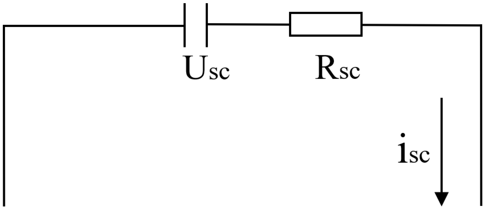
2.2. Mathematical Model of Supercapacitor

When modeling supercapacitors, it is necessary to simulate the dynamic voltage changes and related performance parameters during charging and discharging. In order to facilitate modeling and analysis, the control circuit is simplified in this paper, and the supercapacitor adopts the classic RC model [16], as shown in Figure 1.

In the Figure 1, $U_{sc}$ is the ideal voltage of the capacitor, V; and $R_{sc}$ is the ohmic internal resistance, $\mathsf{\Omega }$. The formula for calculating the output voltage of the supercapacitor is as follows:

$$U_{osc}=U_{sc}-i_{sc}{R}_{sc}$$

(4)

where, $U_{osc}$ is the output voltage of the supercapacitor, V.

The relationship between supercapacitor voltage and current is as follows:

$$i_{sc}=-C\frac{d{U}_{sc}}{dt}$$

(5)

where, $C$ is the supercapacitor capacity, F; $i_{sc}$ is the current, A.

The power $P_{scout}$ at the output of the supercapacitor is calculated as follows:

$$P_{scout}=U_{\mathrm{o}sc}{i}_{sc}-i_{sc}{}^2{R}_{sc}^{}$$

(6)

The state of charge of a supercapacitor is expressed as follows:

$$SO{C}_u=\frac{\frac{1}{2}C{U}_{osc}^2}{\frac{1}{2}C{U}_{\max }^2}=\frac{U_{osc}^2}{U_{\max }^2}$$

(7)

where, $SO{C}_u$ is the state of charge of the supercapacitor.

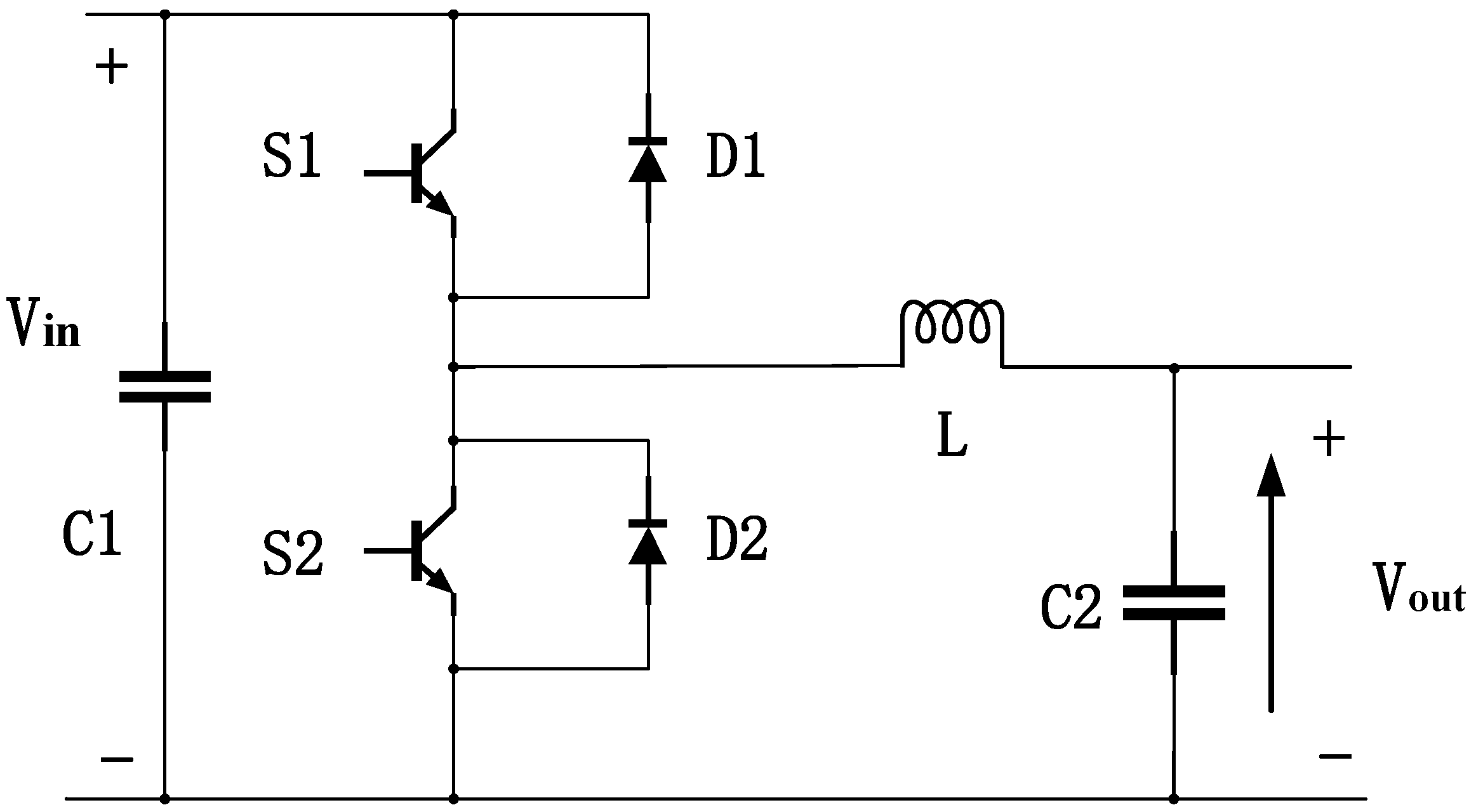
2.3. Bidirectional DC/DC Model

The bidirectional Buck-Boost DC/DC converter can realize the bidirectional flow of energy; it is an important device for adjusting the input and output voltage of the supercapacitor in the composite energy source. Its main function is to adjust the charge and discharge current of supercapacitor, reduce the fluctuation range of terminal voltage, and improve the working efficiency of composite energy source [17]. Its simplified circuit diagram is shown in Figure 2.

In Figure 2, $V_{in}$ is the input voltage, V; $V_{out}$ is the output voltage, V; S1 and S2 are the IGBT switches; L is the inductor; and C1 and C2 are the capacitors. When the energy is transferred from the left to the right, the converter is equivalent to a buck DC voltage converter, and when the energy is transferred from the right to the left, it is equivalent to a boost DC voltage converter.

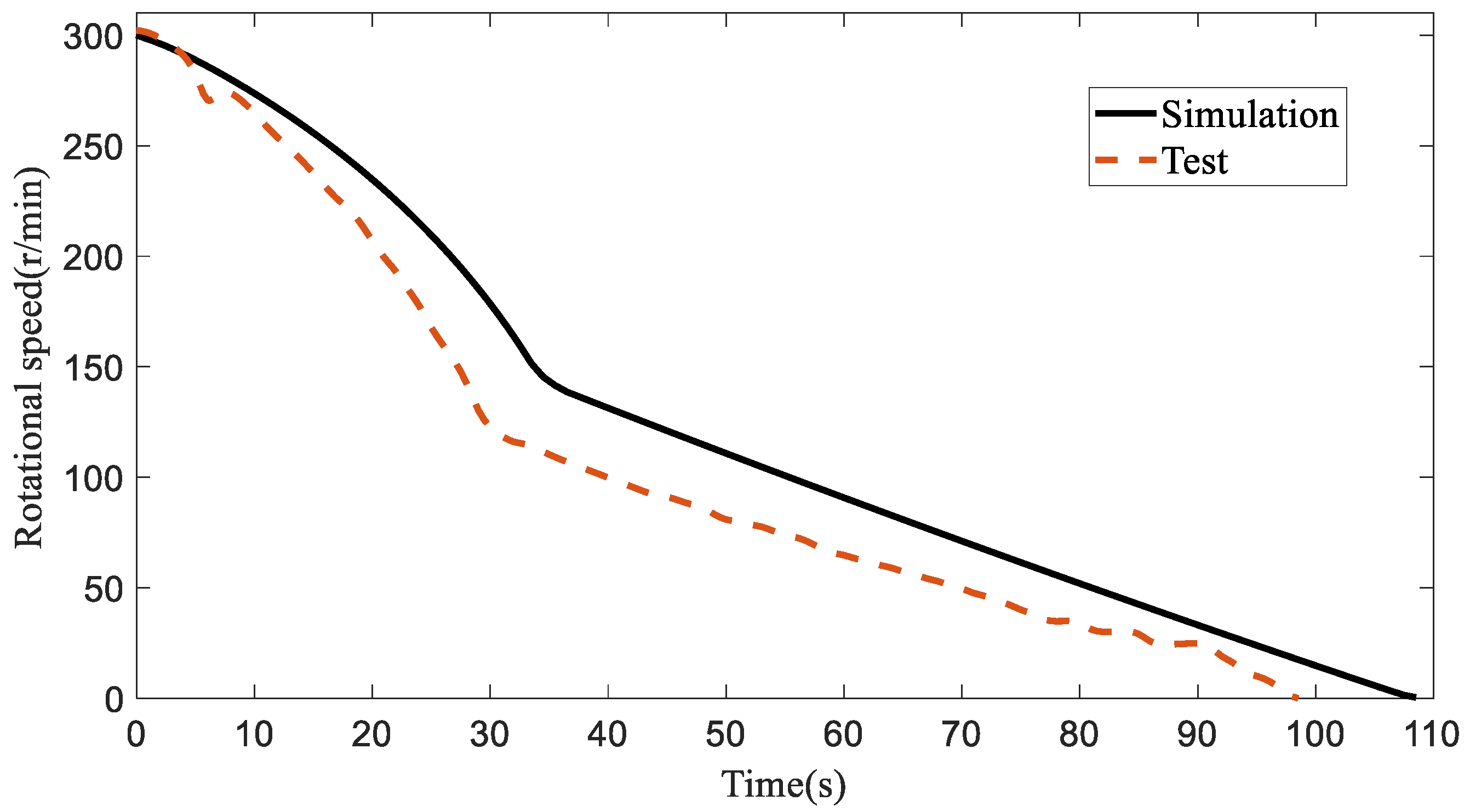
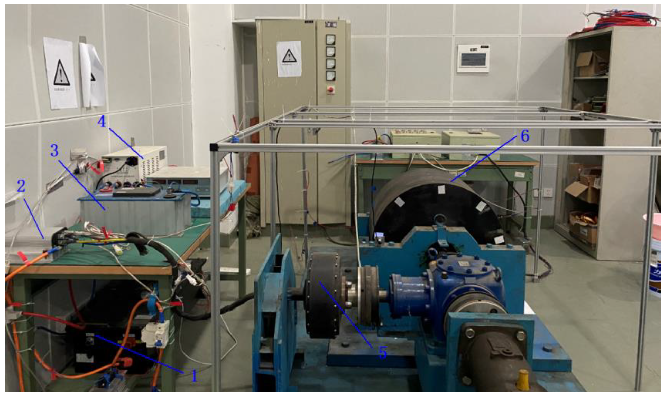
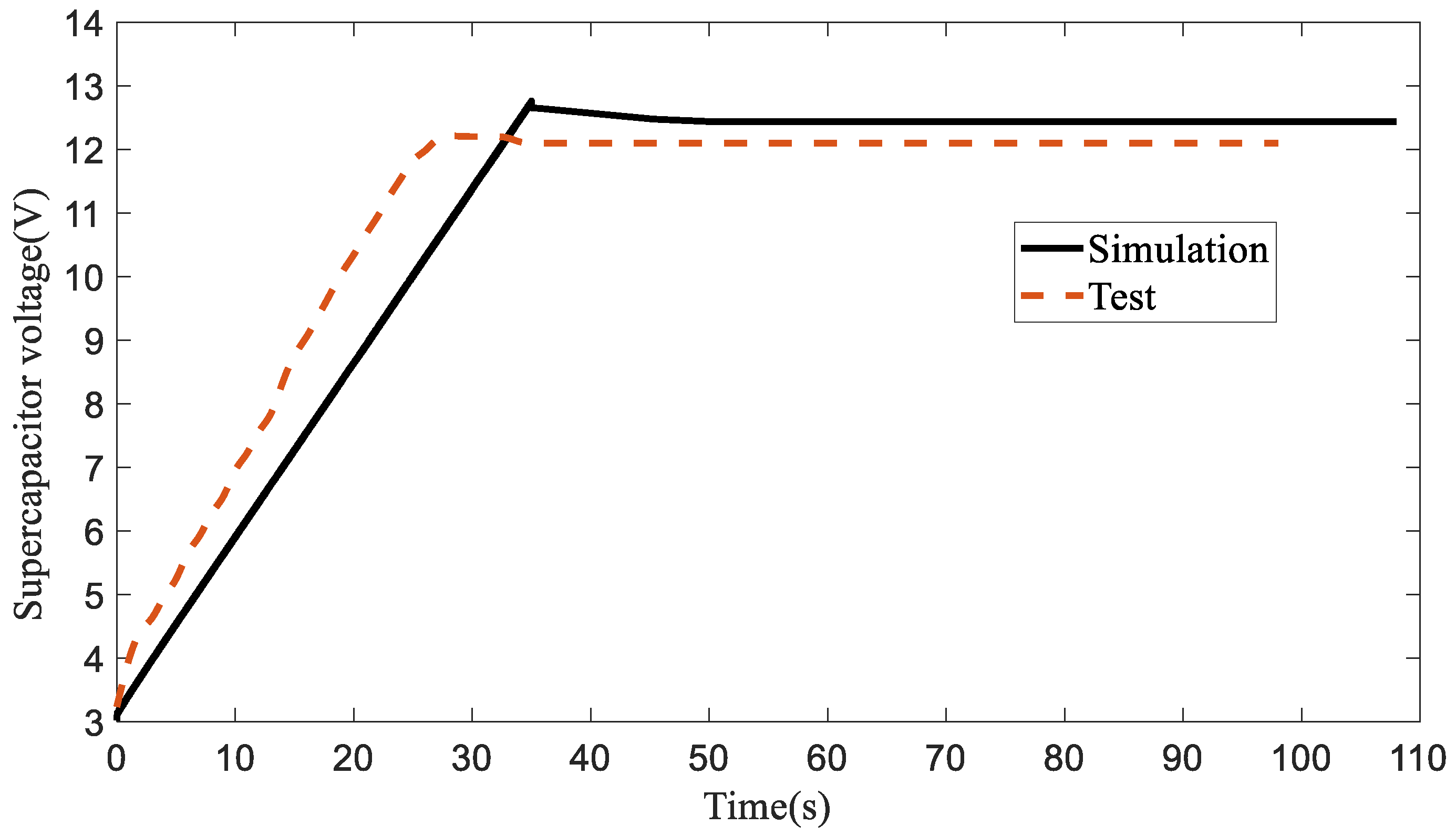
2.4. Simulation and Verification of HERBS

The inertial kinetic energy of the vehicle during braking is simulated by the flywheel, and a HERBS simulation model consisting of flywheel, supercapacitor, bidirectional DC/DC converter and motor is built in MATLAB software, and the changes of each parameter in the braking energy recovery process are studied by simulation. Among them, the motion equation of flywheel is as follows [18]:

$$E_f=\frac{1}{2}{J}_f{\left({\omega }_0^2-{\omega }_1^2\right)}^{}$$

(8)

where, $E_f$ is the kinetic energy change in the flywheel, J; $J_f$ is the rotational inertia of the flywheel as it rotates around the bearing, kg·m²; ${\omega }_0$, ${\omega }_1$ are the rotational speeds of the flywheel before and after braking, rad/s.

In order to verify the accuracy of the established simulation model, a HERBS test-bench consisting of supercapacitors, bidirectional DC/DC converters, power batteries, motor controllers, brushless DC motors and flywheels was built, as shown in Figure 3. The key parameters of the test-bench are as follows: the rated voltage of the supercapacitor is 48 V, and the capacitance is 165 F; the rated voltage of the motor is 72 V, the rated power is 8 KW, and the rated speed is 1440 r/min; the moment of inertia of the flywheel is 45.3 kg·m²; the resistance of the ripple resistance is 0.4 Ω, and the power is 5 KW.

The braking energy recovery test was carried out when the flywheel speed was 300 r/min, and the supercapacitor charging current was set to 40 A during the test. Figure 4 and Figure 5, respectively, show the comparison of the simulation and test of the supercapacitor voltage and flywheel speed in the process of braking energy recovery. It can be seen that the simulation results are basically consistent with the test, thus indicating that the established simulation model is accurate. Among them, the simulation result of supercapacitor voltage is slightly larger than the test value. The main reasons are as follows: the simulation ignores the influence of frictional resistance and air resistance between bearings during the rotation of flywheel, while the test causes some kinetic energy to be consumed due to the existence of frictional resistance and air resistance; the simulation ignores the influence of the charging efficiency of DC/DC, and the conversion efficiency of the DC voltage converter in the test is affected by the voltage ratio and power, and the charging efficiency cannot reach 100%.

Among them, the flywheel speed curve has a high slope at the beginning and a low slope at the end of a long period. Analyzing the reasons, the larger slope occurs in the process of braking energy recovery, and the smaller slope occurs after the braking energy recovery stops. Since the power of the bidirectional DC voltage converter is equivalently changed during operation, that is, the input power is always equal to the output power. However, as the flywheel speed decreases, the input power of the DC voltage converter gradually decreases, and the voltage of the supercapacitor increases due to charging, resulting in a higher demand for the output power of the DC voltage converter. Once the output power demand of the DC voltage converter is greater than the input power of the DC voltage converter, and the DC voltage converter will automatically cut off the charging. At this time, the current generated by the motor can no longer be recovered to the super capacitor, and the braking torque generated in the motor decreases, so in the second half, the speed of the flywheel speed decreases slowly.

3. Establishment of Vehicle Model of HERBS

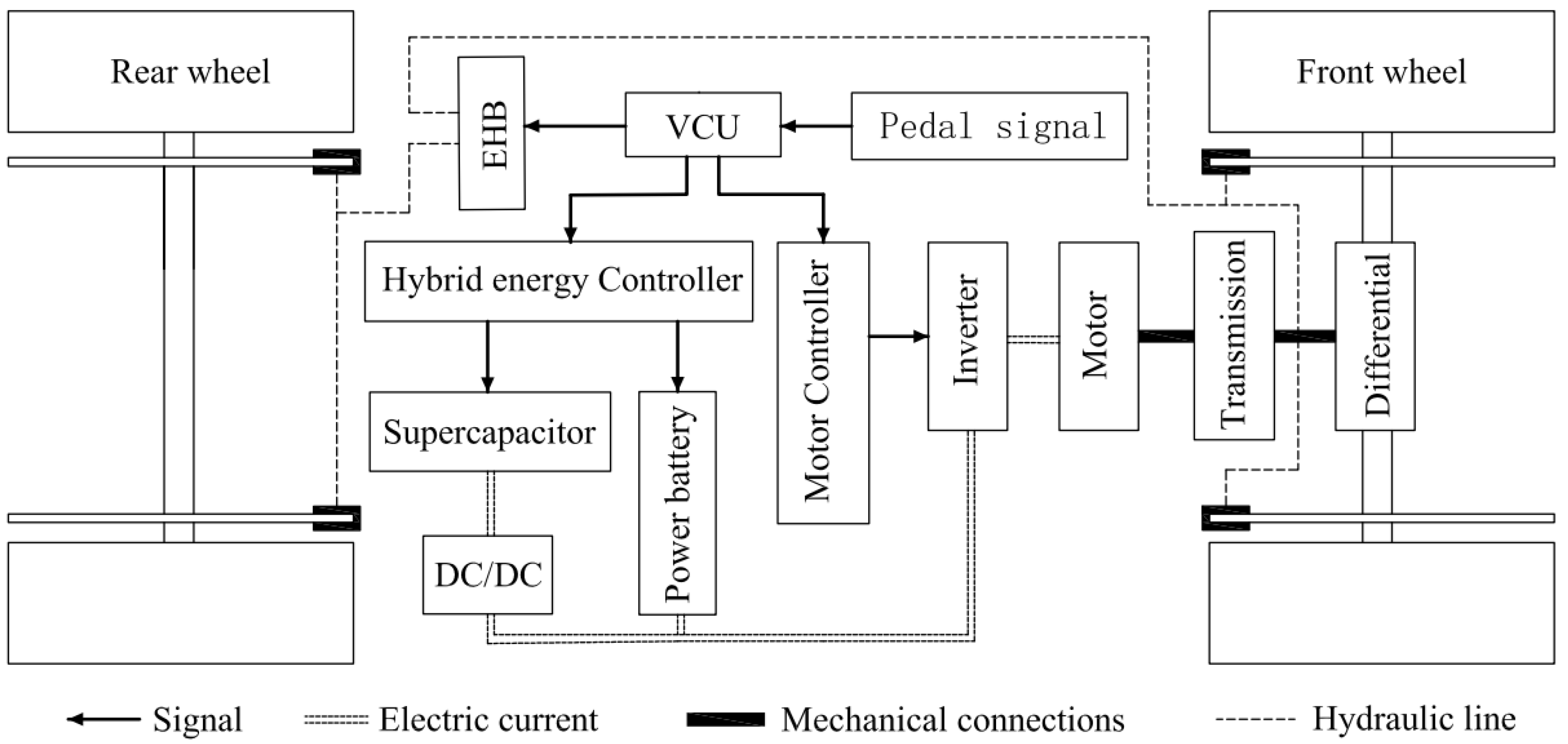
3.1. Working Principle of HERBS

The HERBS in this paper consists of supercapacitor, DC/DC, power battery, motor control system and motor. The motor is connected to the front drive shaft through the differential to provide power for the vehicle. The supercapacitor is connected with the hybrid energy controller, which controls whether the supercapacitor is charged and discharged through the hybrid energy controller; the supercapacitor can store the feedback braking energy, and together with the vehicle power battery as an energy storage device, provide energy for the electric vehicle. The working principle is shown in Figure 6.

When the vehicle’s brakes are active, the VCU of the whole vehicle transmits control information to the motor control unit according to the brake pedal signal and the vehicle speed at this time, and the motor control unit controls the inverter to make the brushless DC motor rotate with the wheel, and the permanent magnet rotor cuts the stator coil. At this time, the brushless DC motor is transformed into a generator to convert the kinetic energy of the flywheel into electric energy and store it in the supercapacitor, thereby realizing the recovery of braking energy. At the same time, the force received by the rotor in the magnetic field will also be fed back to the wheels through the transmission system, thus generating the required regenerative braking force. In the process of braking energy recovery, the motor control unit plays the role of a full bridge rectifier circuit, converting the three-phase alternating current generated by the brushless DC motor into direct current, and then converts it through the bidirectional DC/DC converter and charges it into the supercapacitor. When the vehicle starts or accelerates, the VCU controller of the whole vehicle receives the pedal acceleration signal. At this time, the demand power is large, and the supercapacitor is required to assist in acceleration, and the supercapacitor is connected in parallel with the power battery through the DC/DC converter, so that the motor has a strong driving force to drive the vehicle forward or accelerate, while protecting the battery from large current impact.

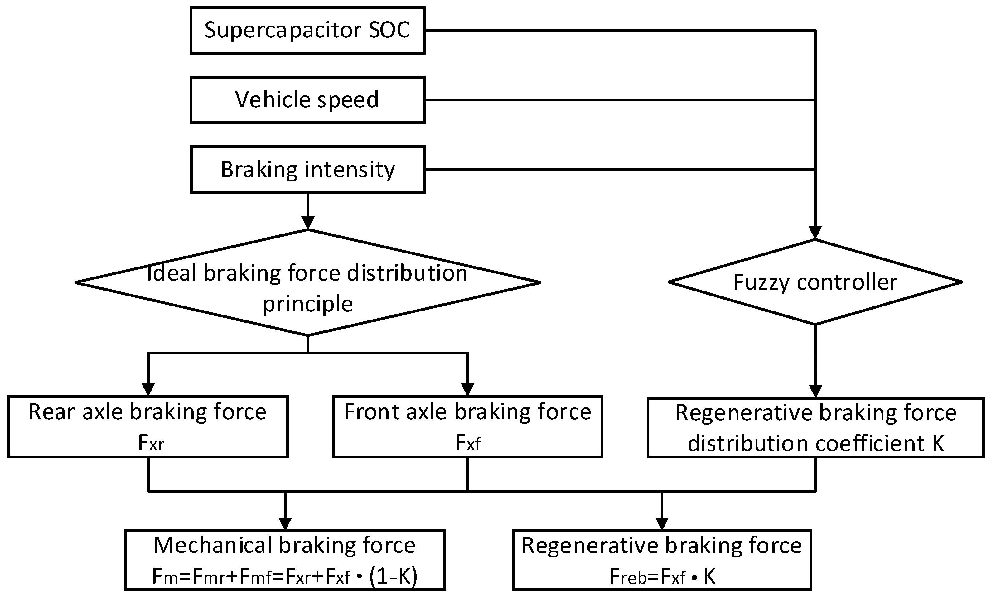
3.2. Distribution Strategy Design of Brake Force

In this paper, the front-wheel drive vehicle is studied; the braking force distribution strategy is shown in Figure 7. When braking, the front and rear axle braking forces are distributed according to the braking intensity. At the same time, the fuzzy controller calculates the regenerative braking force distribution coefficient K according to the input supercapacitor SOC, vehicle speed and braking intensity, and completes the distribution of the front axle regenerative braking force F_reb and mechanical braking force F_mf. Among them, the braking intensity $z$ is expressed as the ratio of the vehicle’s braking deceleration $a_x$ to the gravitational acceleration $g$, that is, $z=\left|a_x\right|/g$, which is an evaluation index of braking efficiency [19].

In order to ensure braking safety, the braking forces of the front and rear axles are distributed according to the ideal braking force distribution principle [20], and the calculation formula is as follows:

$$\begin{array}{l}{F}_{xf}=G\cdot \varphi \cdot (b+z\cdot h_g)/L\\ F_{xr}=G\cdot \varphi \cdot (a-z\cdot h_g)/L\end{array}$$

(9)

where, $F_{xf}$ is the braking force distributed by the front wheels, N; $F_{xr}$ is the braking force distributed by the rear wheels, N; $G$ is the gravity of the vehicle, N; z is the braking intensity; $\varphi$ is the road adhesion coefficient at the front and rear wheels; $a$, $b$ are the distances from the center of mass to the front and rear axles, m; h_g is the height of the center of mass of the vehicle, m; $L$ is the wheelbase, m.

Under the premise of ensuring the braking safety, in order to recover the braking energy as much as possible, a fuzzy controller is built. The vehicle speed, supercapacitor SOC and braking intensity are taken as input variables, and the regenerative braking force distribution coefficient K is taken as output variable. The regenerative braking force and mechanical braking force of the front axle are distributed through fuzzy control rules. The control principles of the fuzzy controller are as follows:

(1)

When the vehicle speed is too high, less braking energy shall be recovered for braking safety; when the vehicle speed is too low, less braking energy is recovered.

(2)

When the supercapacitor SOC is high, the charging efficiency is low, and the braking energy is recovered as little as possible; when the supercapacitor SOC is low, the charging efficiency is high and the energy can be recovered as much as possible.

(3)

When the braking intensity is too high, energy is not recovered for braking safety; when the braking intensity is low, the recovery of braking energy shall be increased.

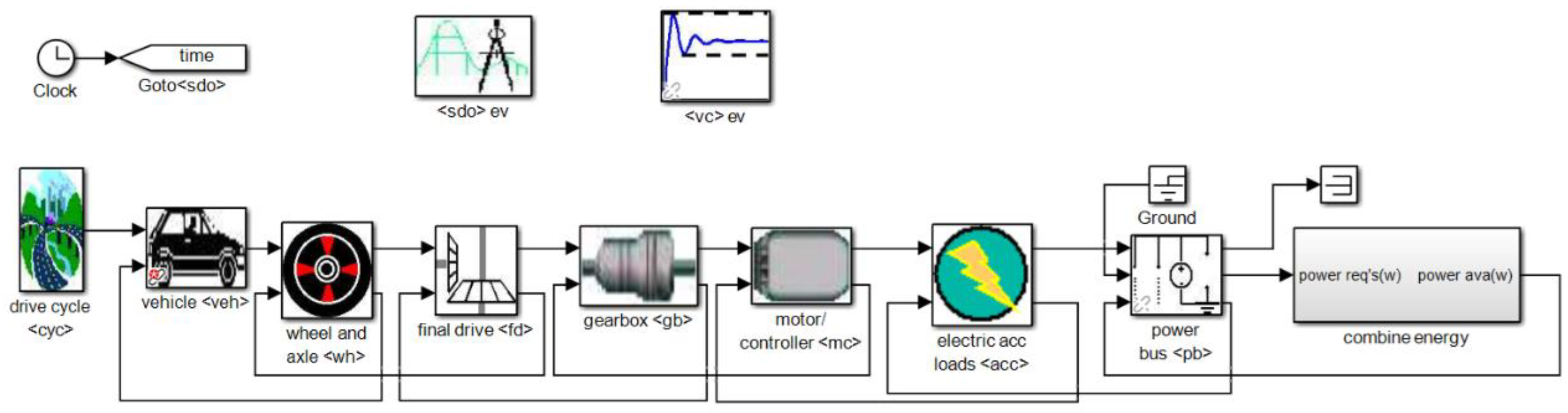
3.3. HERBS Vehicle Model

In the vehicle model of ADVISOR software, modify the power battery model and braking force distribution model of the original vehicle to the hybrid energy model and braking force distribution model established in this paper, and modify the vehicle parameters to complete the establishment of the vehicle model, as shown in Figure 8.

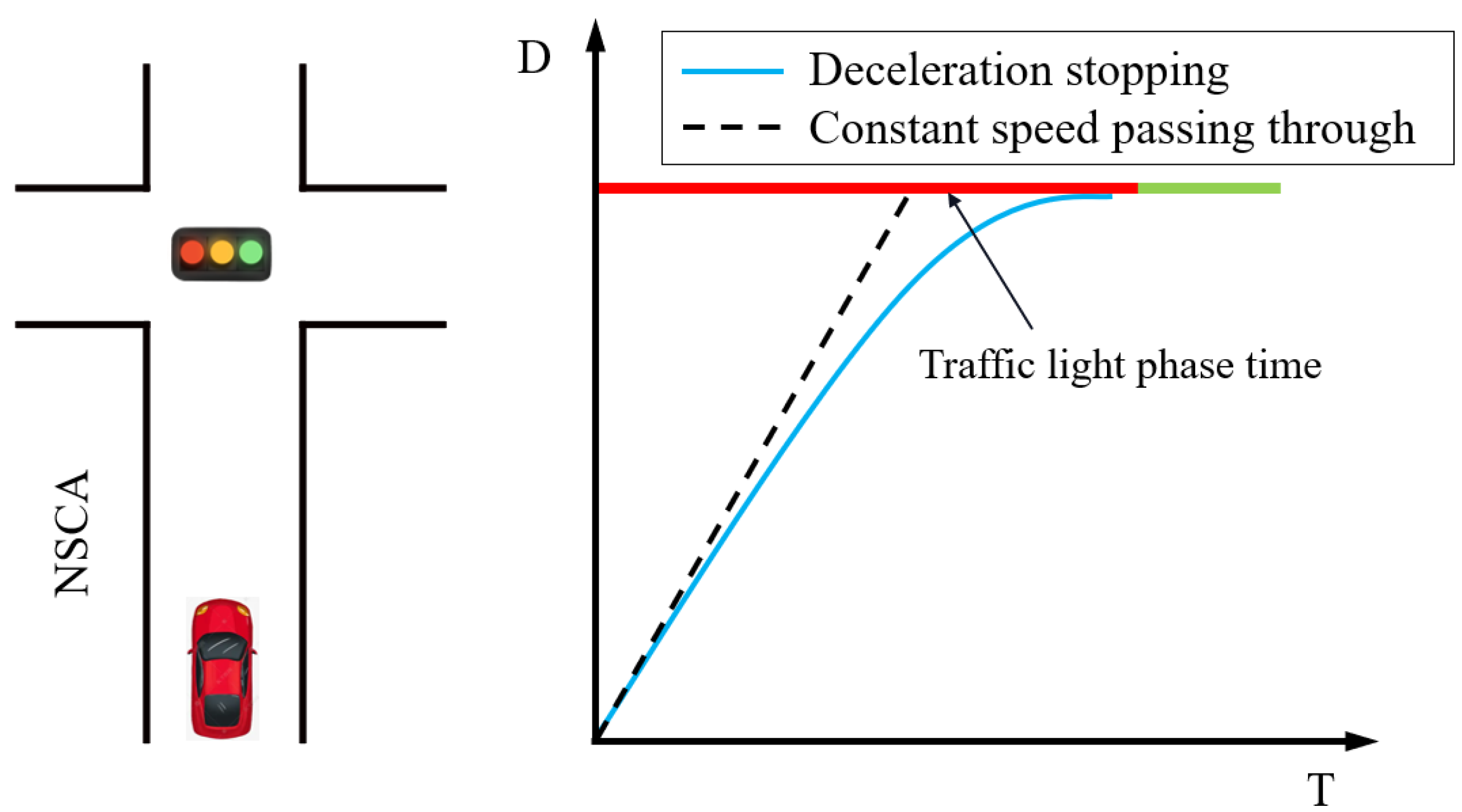
4. Analysis of the Traffic Characteristics of a Single Vehicle in the near Signal Control Area

According to China’s traffic laws, vehicles must pass through the stop line within the green-light and yellow-light cycle. If they encounter a red-light, they need to stop until the next green-light cycle. This chapter studies the braking process of a single vehicle at the near signal control area (NSCA), with the aim of recovering as much braking energy as possible. When the vehicle drives into the NSCA and needs braking, the on-board computer performs the braking control so that the braking energy recovery is maximized. As the external traffic environment interference factors are complex and changeable, in order to study the above problems more pertinently, the following assumptions are made [21]:

(1)

Ignore the impact of pedestrians and non-motor vehicles on the study vehicles;

(2)

The main research object is a single signalized intersection, without considering the impact of other intersections;

(3)

It mainly studies the straight driving conditions of vehicles. The vehicle lane changing conditions are not taken into account, and the problem of traffic conflict is ignored;

(4)

Classify the yellow-light as the red-light, which means that forbidden for vehicles to cross the stop line when the yellow-light is on.

Based on the above assumptions, the driving characteristics of a single vehicle in the NSCA are analyzed. Firstly, the space-time characteristics of a single vehicle in the NSCA are analyzed. According to the signal light phase and the distance from the vehicle to the stop line, the speed changes are divided into four categories: constant speed passing through, acceleration passing through, deceleration passing through and deceleration stopping. This paper mainly studies the behavior under braking conditions, so it only analyzes the two conditions of deceleration passing through and deceleration stopping. Next, the movement behavior of the vehicle during braking in the NSCA is analyzed through the schematic diagram. In the diagram, the ordinate represents the driving distance of the vehicle, the abscissa represents the driving time of the vehicle, and the red and green line segments represent the traffic light phase time during the driving process.

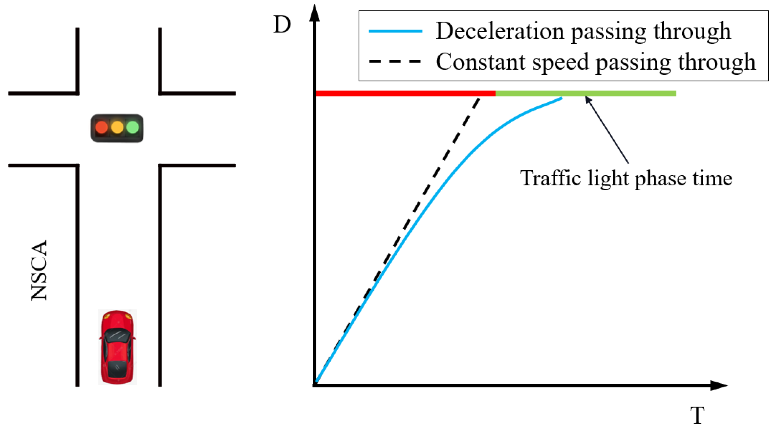
4.1. Deceleration Passing through Condition

When the vehicle enters the NSCA, the phase of the signal light at this time is red, and it takes a certain time to turn to the green-light. If the vehicle continues to drive at a constant speed, it cannot pass through the stop line, and it is necessary to appropriately decelerate in advance to ensure that drive passing through the stop line after the signal light turns green, avoiding stopping and improving traffic efficiency. The schematic diagram of deceleration passing through is shown in Figure 9 below.

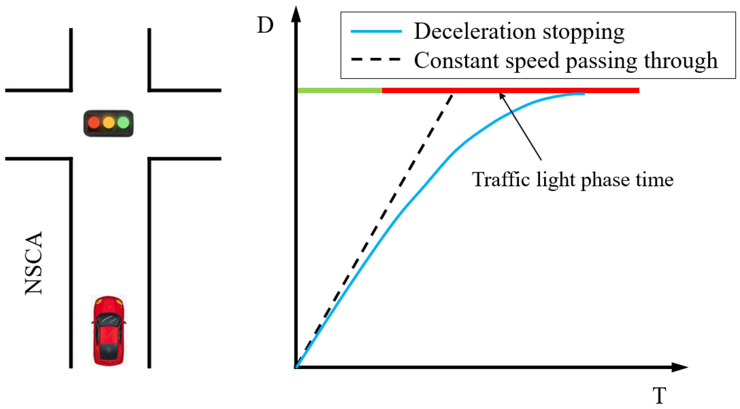
4.2. Deceleration Stopping Condition

There are two cases of deceleration stopping. One case is to decelerate stopping for if the vehicle enters the NSCA when the speed is moderate, and the phase of the signal light is green, but the green-light is about to change to red. Even if the vehicle accelerates, it cannot pass through the stop line before the green-light turns red, and it can only stop and wait for the next green-light to pass through. The schematic diagram of stopping at the green phase is shown in Figure 10 below.

The other case of deceleration stopping situation is when the vehicle enters the NSCA at a moderate or fast speed, the signal is red and has a long time remaining, even if the vehicle is decelerating, it will still drive, passing through the stop line within the red phase, which is a violation of traffic regulations. In this case, the vehicle must stop in front of the stop line and wait for the next green phase before starting to pass through. The diagram of stopping at a red-light phase is shown in Figure 11 below.

We comprehensively analyzed the driving situation of the vehicle in the NSCA, and found that there is generally more braking in this area; the speed of the vehicle entering the NSCA is different, traffic light phase situation and remaining time are also randomly met, in the limited conditions of signal lights and vehicle movement, the decision regarding how to brake will greatly affect the vehicle braking safety and BERE. Since the deceleration stopping condition at the signalized intersection is the same as the deceleration passing through condition, there are braking situations, and the deceleration stopping conditions are more representative. Therefore, the deceleration stopping conditions at the signalized intersection are modeled and studied next, with the BERE as the goal; the GA is used to optimize the speed trajectory under deceleration stopping conditions.

5. Optimization of Speed Trajectory in NSCA Based on GA

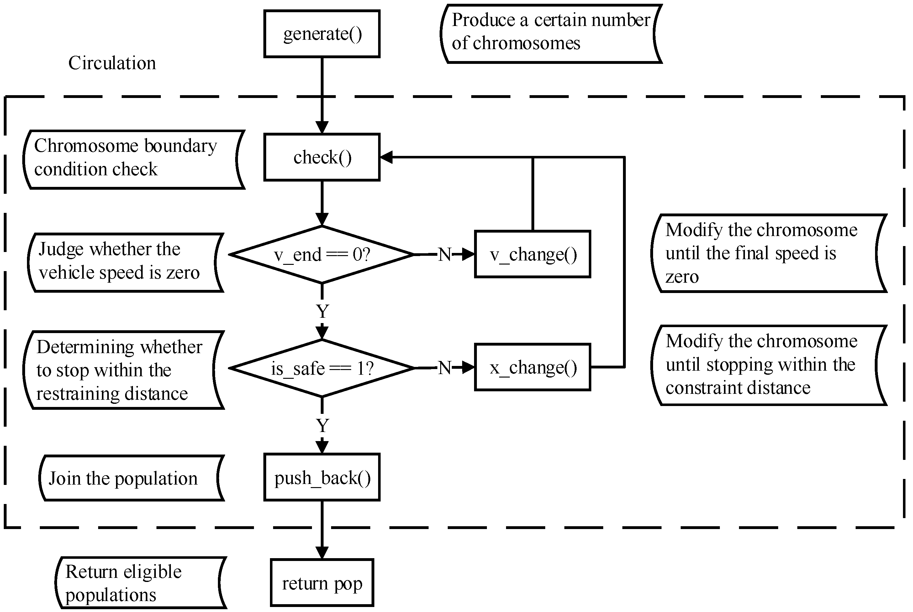
5.1. Establishment of GA Optimization Mathematical Model for Deceleration Stopping

GA is a method for the optimal solution search using the biological evolutionary process of genetic mechanism, and the optimization process is to screen out chromosomes with better fitness from generation to generation according to the procedure of survival of the fittest. The main advantage is that it can directly operate on the research target, without restrictions on derivation and function continuity; it has inherent implicit parallelism and good global optimization capabilities; it adopts a probabilistic optimization method that does not require certain rules, and automatically optimizes search space, and adjusts the search direction adaptively [22,23]. Because the optimization of deceleration stopping in this paper has a certain discreteness and no definite rules, it is more suitable to use GA for optimization.

Deceleration stopping needs to meet in a certain time, less than a certain distance to stop. The constraint distance in the NSCA that is the current position of the vehicle and the distance of the stop line at the signalized intersection; the constraint time that is the red-light phase time, the constraints are shown in the following formula.

$$\{\begin{array}{l}0<x_i\le x_{end}\\ v_{end}=0\\ 0<t_{end}\le t_{red}\end{array}$$

(10)

where, $x_i$ is the total distance traveled by the vehicle in sequence $i$, m; $x_{end}$ is the distance from the current position of the vehicle to the stop line at the signalized intersection, m; $v_{end}$ is the final speed of the vehicle, m/s; $t_{end}$ is the time it takes for the vehicle to stop, s; $t_{red}$ is the remaining time at the red-light, s.

The vehicle speed is solved as follows:

$$v_{end}=v_{\mathrm{int}}-{\displaystyle {\int }_0^{t_{end}}z(t)}dt$$

(11)

Discretizing Equation (11), obtain the formula is as follows:

$$v_{i+1}=v_i-z_i\times g\times t_i$$

(12)

where, $v_{\mathrm{int}}$ is the initial speed of the vehicle, m/s; $v_{\mathrm{i}+1}$ is the speed of the vehicle in the sequence i + 1, m/s; $v_{\mathrm{i}}$ is the speed of the vehicle in the sequence $i$, m/s; $z_{\mathrm{i}}$ is the braking intensity of sequence $i$; $g$ is the acceleration of gravity, m/s²; $t_i$ is the time step of sequence $i$, s.

To solve the vehicle travel time, the formula is as follows:

$$\{\begin{array}{ll}{t}_i=t_{gap}& v_{i+1}>0\\ t_i=\frac{v_i}{z_i\times g}& v_{i+1}\le 0\end{array}$$

(13)

where, $t_{gap}$ is the set fixed time step, s.

To solve the distance traveled by the vehicle, the formula is as follows:

$$x_{end}={\displaystyle {\int }_0^{t_{end}}v(t)dt}$$

(14)

The discretization of Equation (14) is solved to obtain the equation shown below:

$$\{\begin{array}{ll}{x}_{i+1}=x_i+\left(\frac{v_i+v_{i+1}}{2}\right)\times t_i& v_{i+1}>0\\ x_{i+1}=x_i+\frac{v_i^2}{2\times z_i\times g}& v_{i+1}\le 0\end{array}$$

(15)

where, $x_{i+1}$ is the sum of the distance traveled in the sequence i + 1, m.

The fitness function is the sum of the products of the time step of sequence $i$ and the regenerative braking distribution ratio, that is, the sum of the simplified energy distribution, and the optimization goal of the GA is to maximize it.

$$f\left(x\right)=max{\displaystyle \sum }_0^i(t_i\times {\eta }_i)$$

(16)

where, ${\eta }_i$ is the regenerative braking distribution ratio at sequence $i$.

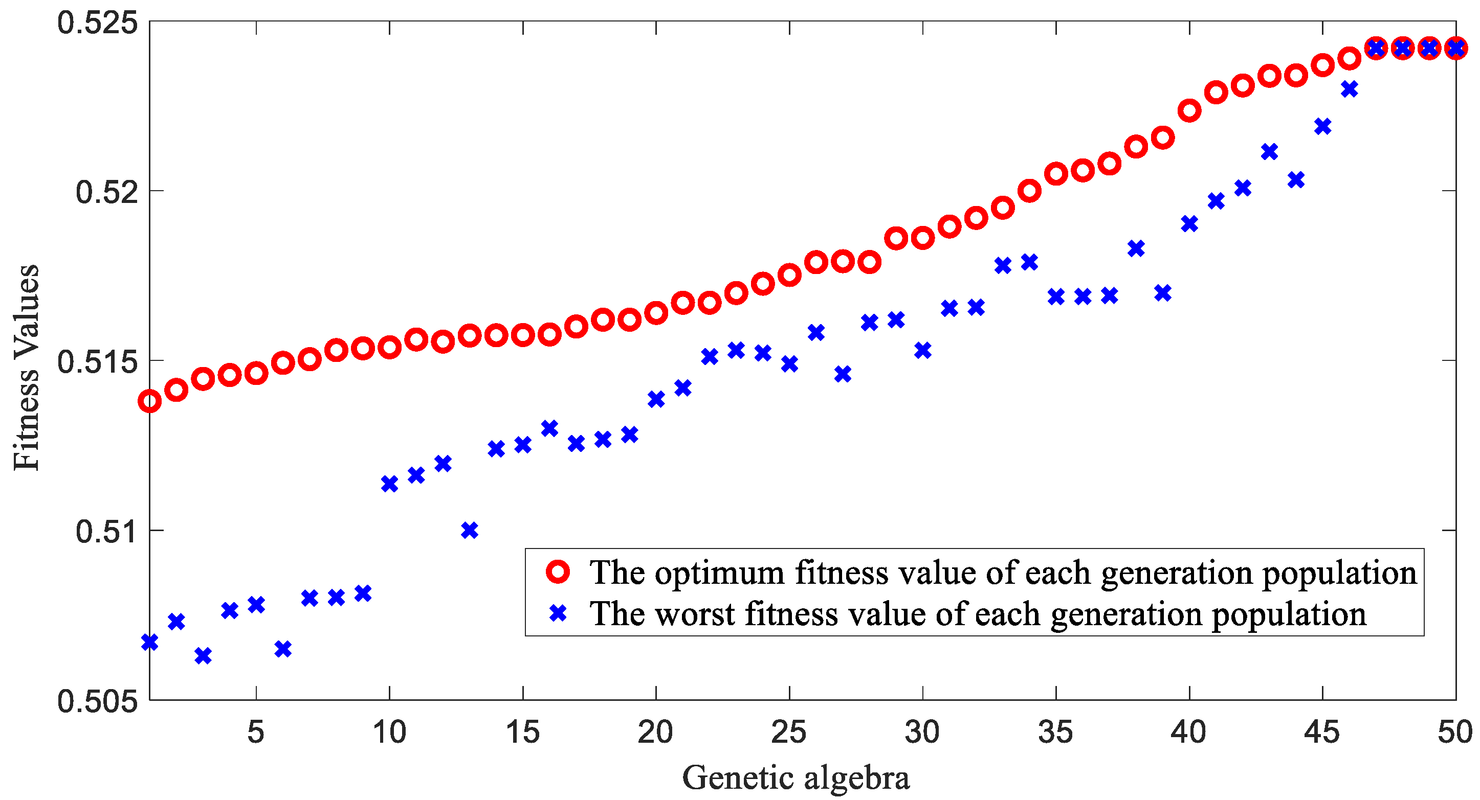
5.2. Deceleration Stopping GA Optimization

Each chromosome in the GA corresponds to a deceleration trajectory, and the fitness function is used to measure the advantages and disadvantages of each chromosome; that is, the sum of the product of the regenerative braking distribution ratio and the braking time, and then the better chromosome is selected to continue to be inherited to the next generation, and some chromosomes are randomly selected for crossover and mutation, so as to prevent the genetic optimization from falling into the local optimal solution. The key steps in the genetic optimization of deceleration stopping are as follows:

Parameter coding: This paper explores the optimal regenerative braking within a certain time and distance. The time is discretized and the floating-point coding method is used, each chromosome represents a deceleration trajectory, and each gene represents the current braking intensity, as shown in Figure 12.

Initial population setting: A certain number of chromosomes are randomly generated, since the optimization process needs to meet the requirements of braking distance and braking time. Therefore, after the randomly generated population, it is necessary to traverse the chromosomes and modify the chromosomes that do not satisfy the conditions to satisfy the constraints. The flowchart is shown in Figure 13.

Details are as follows: After the program enters the generate child function, the check function is used to check the boundary conditions for each chromosome, the check function makes a judgment on the final speed of the vehicle according to equation 11 and returns the $v\_end$ value, and makes a judgment on the distance of the vehicle traveled according to Equation (14) and returns the $is\_safe$ value. If the $v\_end$ value is zero, it means the vehicle final speed is zero; otherwise, the $v\_change$ function (see Equation (12)) needs to be called to modify the chromosome until the vehicle final speed is zero. If the value of $is\_safe$ is one, it means that the vehicle driving distance is less than the safe distance, otherwise, the $x\_change$ function (see Equation (15)) needs to be called to modify the chromosome. When the chromosome meets the boundary condition, it is added to the tail of the population matrix. When all chromosomes in the population have completed the boundary condition detection, the generate function returns the population matrix to the main function.

The fitness function adopts the vehicle model established in Section 3.3, and the parameters of the vehicle are shown in

Table 1. The parameters of the vehicle.

Component	Parameter	Quantity
Mass	kg	1800
Wheel base	m	2.85
Front wheel track	m	1.57
Rear wheel track	m	1.56
Center of gravity	m	0.53
Distance from center of mass to front axle	m	1.254
Distance from center of mass to rear axle	m	1.596
Air drag coefficient	/	0.28
Wheel rolling radius	m	0.32

, and then the GA optimization is finally completed after conventional selection, crossover and variation.

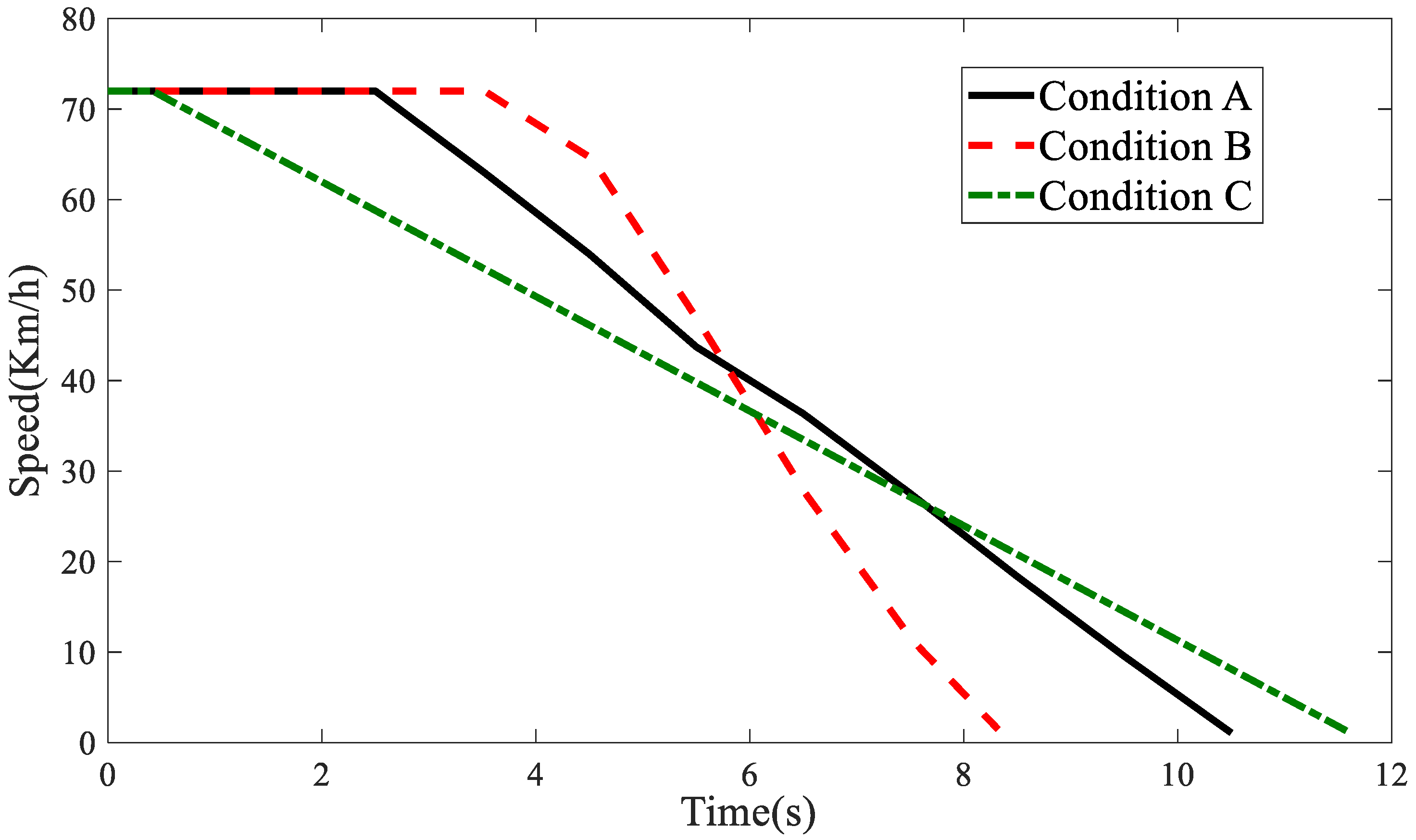
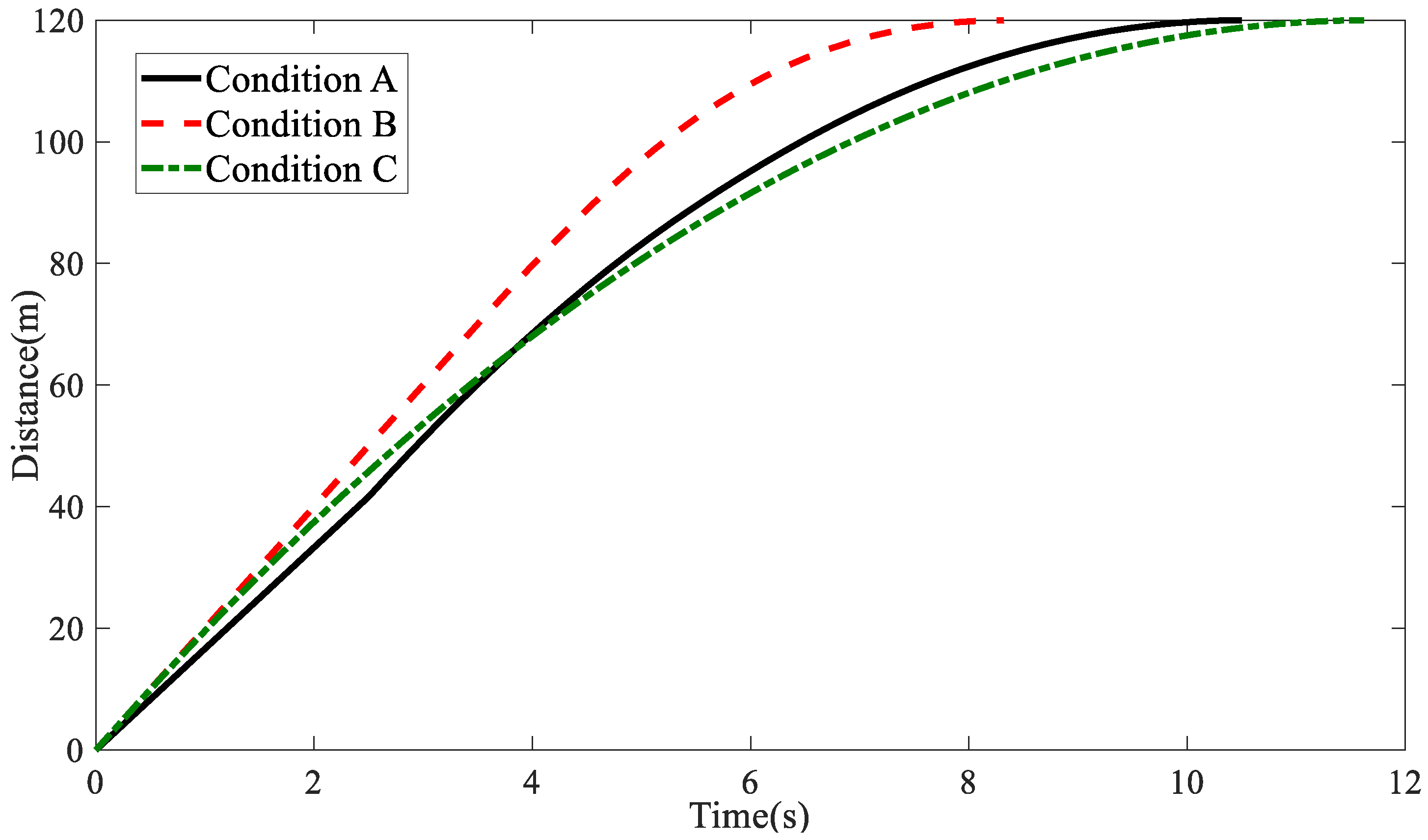
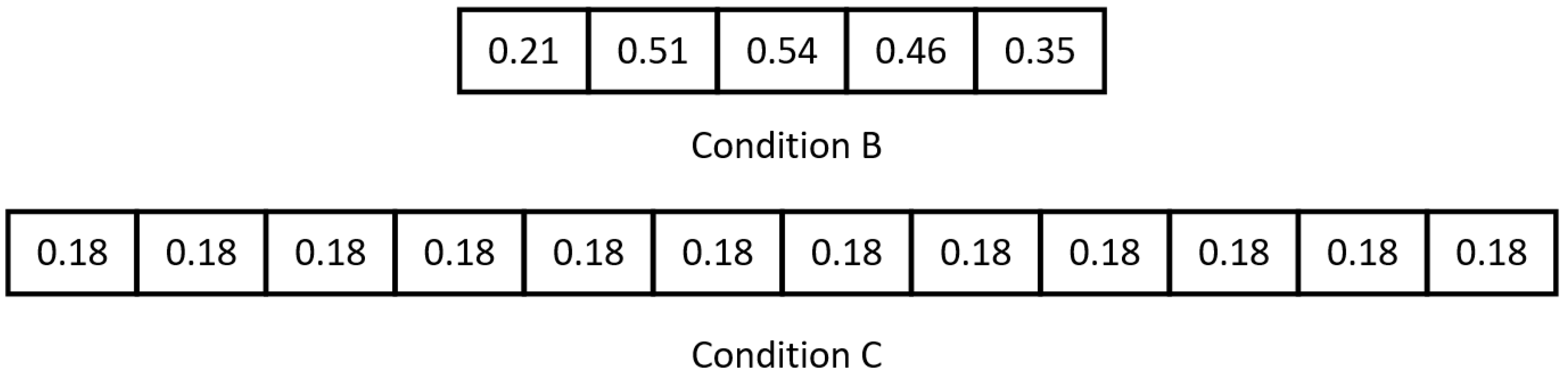
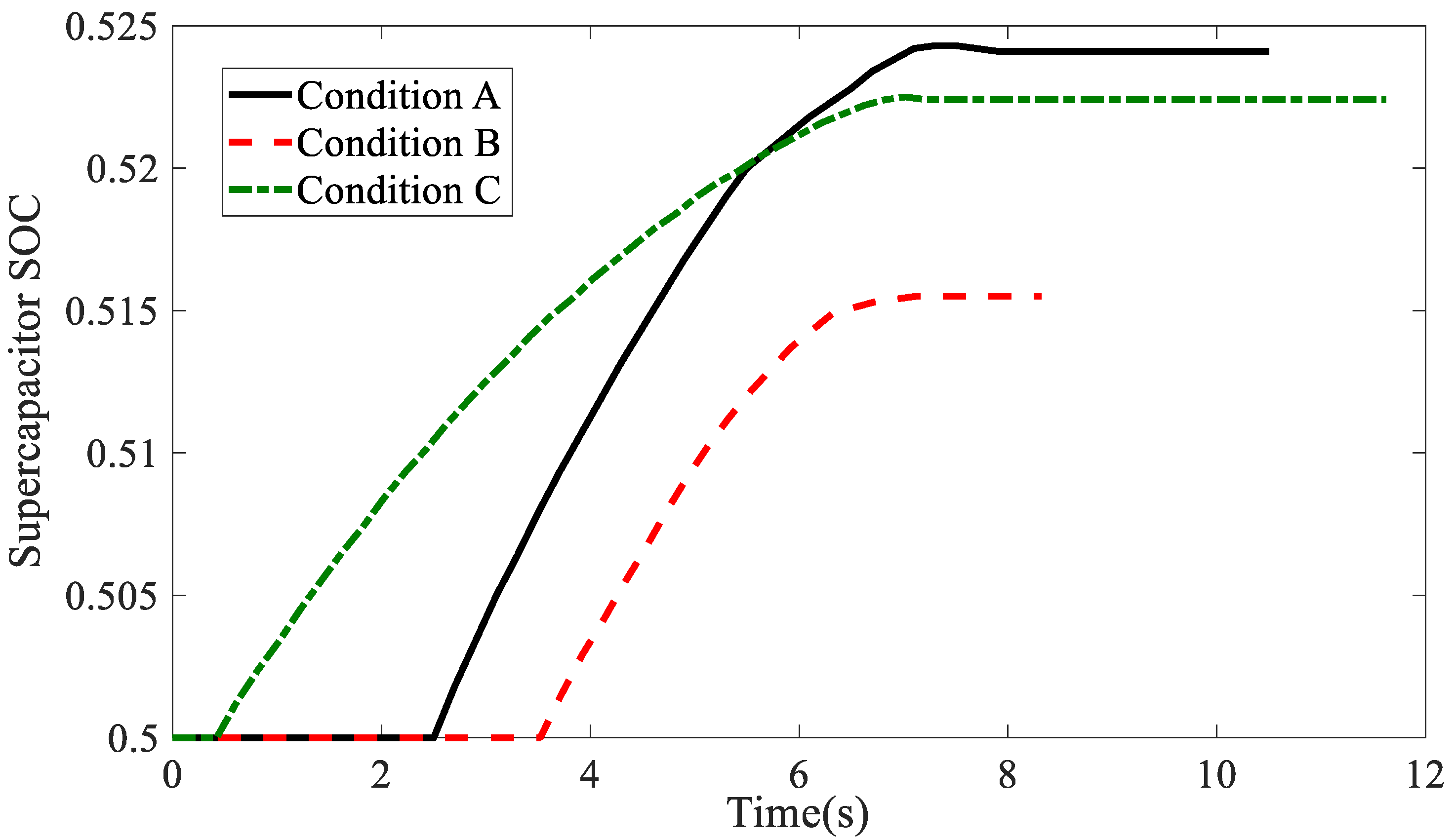
5.3. Comparative Analysis of Simulation Results

The input parameters for the deceleration stopping optimization process are shown in

Table 2. Input parameters for GA optimization of deceleration stopping.

Symbol	Numerical	Unit
$t_{gap}$	1	s
$x_{end}$	120	m
$t_{red}$	20	s
$v_{\mathrm{int}}$	20	m/s

.

After 50 generations of cyclic selection, crossover, and mutation of the GA, the chromosome with the highest fitness value, that is, the optimal braking sequence is generated, as shown in Figure 14. The circular markers in the figure represent the optimal chromosome fitness values, and the fork markers represent the worst chromosome fitness values in each generation of the population. It can be seen that the chromosome fitness of each generation of the population increases as the number of generations increases, until it stops increasing at 47 generations, and the optimal and worst chromosomes are exactly the same, indicating that the GA has found the approximate optimal solution when it reaches the 47th generation.

Through the optimization results in Figure 14, the optimal chromosome, i.e., optimal braking sequence is obtained as shown in Figure 15. It means that braking according to the gene sequence of this chromosome can obtain the most BERE within the constraints.

In this section, within the distance of $x_{end}$ = 120 m, the braking sequence of the optimal chromosome is obtained by GA optimization. For comparison, the braking sequence is defined as condition A, and the two chromosomes shown in Figure 16 are selected as condition B and condition C. Condition B is high-intensity braking, used to simulate the emergency braking situation when the inexperienced driver encountering red-light; condition C is uniform deceleration and low-intensity braking, used to simulate the experienced driver encountering red-light let the vehicle slide. Because the braking intensity of each condition is different, in order to ensure that the final driving distance is the same, it is defined that the vehicle runs at a constant speed when no braking is performed in the early stage. Since the braking energy is not recovered when running at a constant speed, it has no influence on the research results. Next, through vehicle braking simulation in ADVISOR software, the BERE and braking stop time under three working conditions are compared, so as to verify the optimization results in this paper. Among them, the BERE is evaluated by the final value of the supercapacitor SOC. Under the condition of the same initial value of the supercapacitor SOC, the larger the final value at the end of the simulation, the more braking energy is recovered.

Figure 17, Figure 18 and Figure 19 are the curves of the vehicle speed, displacement, and supercapacitor SOC with time during the braking process. it can be seen that with each working condition, the final driving distance are the same; only the vehicle driving time and braking time are different. Condition C driving time is the longest, condition A is the second, condition B is the shortest. Analyzing the reasons, condition C is a low-intensity braking, the braking time is relatively long, and the constant speed driving time in the early stage is relatively small, resulting in a relatively long total driving time. Condition B is high-intensity braking, the braking time is relatively short, and the constant speed driving time in the early stage is relatively long, so the total driving time is relatively short. Condition A has moderate uniform driving time and braking time, so the driving time of the vehicle is also moderate. By comparison, it shows that the driving time from the starting position to the stop line in front of the signal light is moderate in condition A, and the braking time of the vehicle is not deteriorated due to the optimization of the BERE.

Table 3. Variation in supercapacitor SOC under different conditions.

Conditions	Supercapacitor SOC Initial Value	Supercapacitor SOC Final Value	Change Amount	Difference with Condition A
Condition A	0.5	0.5243	0.0243	--
Condition B	0.5	0.5155	0.0155	−36.21%
Condition C	0.5	0.5224	0.0224	−7.82%

shows the comparison of the amount of variation in supercapacitor SOC under different conditions. Through comparison, it can be seen that the supercapacitor SOC of condition A has the largest change, which is 36.21% higher than Case B and 7.82% higher than Case C. This indicates that the BERE of condition A is the highest, and from the previous analysis, condition A has moderate travel time from the beginning to the vehicle stopping down, which also meets the requirement of signalized intersection traffic efficiency. Although the braking time of condition B is the shortest, but the BERE is the lowest, resulting in too high energy consumption of the whole vehicle; the BERE of condition C is improved compared with condition B, but the braking time is too long, which will easily lead to traffic jams at signalized intersections, thus reducing the traffic efficiency of signalized intersections.

In summary, the BERE during deceleration stopping at a single signalized intersection after speed trajectory optimization is 36.21% higher than that of inexperienced driver and 7.82% higher than that of experienced driver, and the braking time duration is moderate. Thus, it shows that the optimal speed trajectory control method based on BERE designed in this paper can well solve the energy consumption problem and passing rate problem of signalized intersections.

6. Conclusions

(1)

Based on the characteristics that connected automated vehicle can communicate with roadside facilities and regional center control systems in real-time, a GA optimization model for the deceleration stopping of electric vehicle HERBS is built. Taking the obtained signal light status and timing information as constraints, and the BERE as the optimization objective, speed trajectory of the autonomous vehicle equipped with the regenerative braking system is optimized at the signalized intersection and BERE and energy consumption are improved greatly.

(2)

The proposed speed trajectory planning method is also applicable for the situation of signalized intersection by deceleration passing through, for both passage efficiency and BERE are favorable, and for reducing the energy consumption.

(3)

Influence of other vehicles in the trip and their effects on the speed trajectory planning, based on the BERE under multi-vehicle environments, should be further investigated in future work.

References

1. Kamalanathsharma, R.K.; Rakha, H.A.; Yang, H. Networkwide Impacts of Vehicle Ecospeed Control in the Vicinity of Traffic Signalized Intersections. Transp. Res. Rec. J. Transp. Res. Board 2015, 2503, 91–99. [Google Scholar] [CrossRef]
2. Bartoletti, S.; Masini, B.M.; Martinez, V.; Sarris, I.; Bazzi, A. Impact of the Generation Interval on the Performance of Sidelink C-V2X Autonomous Mode. IEEE Access 2021, 9, 35121–35135. [Google Scholar] [CrossRef]
3. Song, Z.; Song, K.; Zhang, T. State-of-the-Art and Development Trends of Energy Management Strategies for Intelligent and Connected New Energy Vehicles: A Review. SAE Tech. Pap. 2019. [Google Scholar] [CrossRef]
4. Wang, Z.; Wu, G.; Barth, M. Cooperative Eco-Driving at Signalized Intersections in a Partially Connected and Automated Vehicle Environment. IEEE Trans. Intell. Transp. Syst. 2020, 21, 2029–2038. [Google Scholar] [CrossRef] [Green Version]
5. Yang, H.; Rakha, H.; Ala, M.V. Eco-Cooperative Adaptive Cruise Control at Signalized Intersections Considering Queue Effects. IEEE Trans. Intell. Transp. Syst. 2016, 18, 1575–1585. [Google Scholar] [CrossRef]
6. Cruz-Piris, L.; Lopez-Carmona, M.A.; Marsa-Maestre, I. Automated optimization of Intersections using a genetic algorithm. IEEE Access 2019, 7, 15452–15468. [Google Scholar] [CrossRef]
7. Jinquan, G.; Hongwen, H.; Jianwei, L.; Qingwu, L. Real-time energy management of fuel cell hybrid electric buses: Fuel cell engines friendly intersection speed planning. Energy 2021, 226, 120440. [Google Scholar] [CrossRef]
8. Dong, H.; Zhuang, W.; Chen, B.; Lu, Y.; Liu, S.; Xu, L.; Pi, D.; Yin, G. Predictive energy-efficient driving strategy design of connected electric vehicle among multiple signalized intersections. Transp. Res. Part C 2022, 137, 103595. [Google Scholar] [CrossRef]
9. Wei, X.; Leng, J.; Sun, C.; Huo, W.; Ren, Q.; Sun, F. Co-optimization method of speed planning and energy management for fuel cell vehicles through signalized intersections. J. Power Sources 2022, 518, 230598. [Google Scholar] [CrossRef]
10. Liu, X.G.; Wang, H.N.; Wang, J.W.; Hao, L. Speed Control Strategy and Optimization of Signalized Intersection in Network Environment. J. Transp. Syst. Eng. Inf. Technol. 2021, 21, 82–90. [Google Scholar]
11. Cheng, Y.; Zhao, J.Y.; Wang, L. Conflict Resolution Model Based on Multi-vehicle Cooperative Optimization at Intersections. J. Transp. Syst. Eng. Inf. Technol. 2020, 20, 205–211. [Google Scholar]
12. Zhang, B.; Guo, G.; Wang, L.Y.; Wang, Q. Vehicle speed planning and control for fuel consumption optimization with traffic light state. Acta Autom. Sin. 2018, 44, 461–470. [Google Scholar]
13. Sun, C.X.; Mo, B. Design of Control System of Brushless DC Motor Based on DSP. In Proceedings of the 2010 Intelligent Computation Technology and Automation (ICICTA), Changsha, China, 11–12 May 2010; pp. 11–14. [Google Scholar]
14. Yue, X.L.; Bai, P. Modeling and simulation of brushless DC motor control algorithm based on matlab. Syst. Simul. Technol. 2019, 15, 120–125. [Google Scholar]
15. Ji, Z.C.; Shen, X.Y.; Jiang, J.G. A novel method for modeling and simulation of BLDC system based on matlab. J. Syst. Simul. 2003, 15, 1745–1749. [Google Scholar]
16. Li, H. Study on Control Strategy of Electric driving and Regeneration Braking for Pure Electric Vehicles. Ph.D. Thesis, Dalian University of Technology, Dalian, China, 2018. [Google Scholar]
17. Meng, Y.J.; Li, X.N. Research on modeling and control strategy of bidirectional DC/DC converter for compound energy source. Mod. Electron. Tech. 2016, 39, 108–110. [Google Scholar]
18. Li, N.; Ning, X.B.; Wang, Q.C.; Li, J.L. Hydraulic regenerative braking system studies based on a nonlinear dynamic model of a full vehicle. J. Mech. Sci. Technol. 2017, 31, 2691–2699. [Google Scholar] [CrossRef]
19. Yu, F.; Lin, Y. Vehicle System Dynamics; China Machine Press: Beijing, China, 2008. [Google Scholar]
20. Yu, Z.S. Automobile Theory; China Machine Press: Beijing, China, 2002. [Google Scholar]
21. Lei, Z.Y.; Gao, J.P.; Qu, J.K.; Xi, J.G. Economic speed planning with consideration the state of traffic lights. Sci. Technol. Eng. 2020, 20, 7484–7492. [Google Scholar]
22. Lei, Y.J.; Zhang, W.S. MATLAB Genetic Algorithm Toolbox and Its Application; Xidian University Press: Xi’an, China, 2014; pp. 150–240. [Google Scholar]
23. Sun, B.; Jiang, P.; Zhou, G.R. AGV optimal path planning based on improved genetic algorithm. Comput. Eng. Des. 2020, 41, 550–556. [Google Scholar]
Figure 1. Supercapacitor RC Model.
Processes 10 01414 g001
Figure 2. Bidirectional DC/DC converter circuit simplified diagram.
Processes 10 01414 g002
Figure 3. HERBS test-bench. 1. power batteries 2. motor controllers 3. supercapacitors 4. bidirectional DC/DC converters 5. brushless DC motors 6. flywheel.
Processes 10 01414 g003
Figure 4. Variation curve of flywheel speed with time.
Processes 10 01414 g004
Figure 5. Variation curve of supercapacitor voltage with time.
Processes 10 01414 g005
Figure 6. Working principle diagram of HERBS.
Processes 10 01414 g006
Figure 7. Brake force distribution strategy.
Processes 10 01414 g007
Figure 8. Vehicle model of HERBS.
Processes 10 01414 g008
Figure 9. Deceleration passing through.
Processes 10 01414 g009
Figure 10. Green-light phase deceleration stopping.
Processes 10 01414 g010
Figure 11. Red-light phase deceleration stopping.
Processes 10 01414 g011
Figure 12. Brake chromosome diagram.
Processes 10 01414 g012
Figure 13. Establishment flow chart of initial population.
Processes 10 01414 g013
Figure 14. The 50 generations of population fitness values.
Processes 10 01414 g014
Figure 15. The optimal chromosome.
Processes 10 01414 g015
Figure 16. Condition B, C braking sequence.
Processes 10 01414 g016
Figure 17. Vehicle speed with time under different conditions.
Processes 10 01414 g017
Figure 18. Driving distance with time under different conditions.
Processes 10 01414 g018
Figure 19. Supercapacitor SOC with time under different conditions.
Processes 10 01414 g019