An Iterative Backbone Algorithm for Service Network Design Problems

Abstract

Service network design problems arise at airlines, trucking companies, and railroads wherever there is a need to determine cost-minimizing routes and schedules, given resource availability and service constraints. In recent years, the application of consolidation-based service network design in the express service has attracted lots of academic attention due to the rapid growth of the express industry. This paper studies the consolidation-based service network design problem, which jointly determines the commodity flow, vehicle dispatching, and fleet sizing. We propose a mixed-integer optimization model to address the problem and design an efficient iterative backbone algorithm to solve large-scale real-world problems. The numerical results of large-scale instances confirmed that the solution obtained by our proposed algorithm is better than that of the primal model, and the running time taken is less than half that of the general solution approach. The computational study confirmed the effectiveness and efficiency of the proposed algorithm.

1. Introduction

Driven by a booming e-commerce environment, the demand for the express delivery industry has grown continuously. In 2021, global parcel shipments reached 157.9 billion in 2021, up 20.3% from the previous year. The combined number of packages delivered by UPS [1] and FedEx [2] in the United States grew 9% to reach a record 12.2 billion packages. Carrier revenues totaled more than $132 billion, up 18.3% from $107.8 billion in 2020. The growing number of shipments has become one challenge for express delivery service systems, since improving the service level while minimizing costs for a huge transportation network is not an easy task. Service providers apply service network design (SND) models, in general, to solve the tactical planning issues for consolidation-based transportation systems, such as express delivery systems. Due to the huge-scale network structure, it has become impossible to solve it manually. To improve service levels while minimizing the total cost, developing efficient algorithms for solving a large-scale network design problem is necessary.

SND has recently received extensive academic attention [3,4]. Such problems are generally formulated as mixed-integer optimization models that employ integer variables in service selection and continuous variables in commodity flow. SND problems fall into the category of the network design problem, which is applied in many applications [5]. In SND formulations, the arcs of the service network represent services operated by transportation assets, and different commodities must be transported from their origins to destinations in time. There are various service costs associated with varying transportation assets for each service arc. In express delivery service networks, parcels travel through sorting centers one by one for consolidation before reaching the destination, as reflected in Figure 1. The main objective of SND is to develop an operational (or load) plan to meet service requirements while achieving the carrier’s economic or service quality objectives. The planning processes can be determined by solving a large-scale consolidation-based SND problem, and determining the services to be executed and the in-time delivery of commodities. This paper proposes an integer programming model with an iterative backbone algorithm to solve the problem efficiently.

Large-scale SND problems are challenging to solve, since the SND problem is NP-hard [6]. Therefore, it is necessary to develop efficient algorithms to generate better solutions for large-scale applications. In real situations of express delivery, there are cyclical schedules for transportation assets, and thus the design-balanced requirements are employed to utilize assets in circular routes [7]. Later, more effort was dedicated to designing service network schedules while simultaneously considering asset positioning and balancing [8,9]. Only a small amount of effort has been devoted to SND considering consolidation-based large-scale network design problems [10,11]. However, in reality, the service provider must jointly consider the design-balance constraints and fleet size problem in a practical consolidation-based SND scenario. There is still a lack of such works with efficient algorithms to address the issue.

The contribution of this paper is twofold. First, we propose a mixed-integer optimization model for a consolidation-based service network design problem that integrates vehicle dispatching, commodity flow, and fleet sizing. Second, an iterative backbone algorithm is used to solve large-scale real-world problems. A distinguishing feature of the algorithm is that large-scale network applications can be solved efficiently to obtain high-quality solutions.

The remainder of the paper is organized as follows: In Section 2, a brief literature review is elaborated. Section 3 describes the problem and formulates the mathematical programming model. Section 4 provides the details of the proposed solution method, and Section 5 includes the computational study. Finally, Section 6 concludes the study.

2. Literature Review

SND belongs to a general network design problem in transportation planning, logistics, telecommunication, and production systems [12,13,14,15]. The objective of the general network design problem consists of finding a minimum cost network decision, i.e., a network configuration to enable the flow of commodities while minimizing the total cost [16]. The SND addresses the combination problem of multi-commodity flow with the routing network design of transportation assets, which focuses on the tactical routing operations [17,18]. SND problems for various applications are generally formulated as mixed-integer optimization models. Service arcs represent scheduled services, providing capacity for a set of commodities transported over transportation assets. The SND models have been employed in maritime transportation [19], rail transportation [20], land-based long-haul transportation [21], tactical planning of parcel delivery with autonomous vehicles [22,23], air freight parcel delivery [24,25], intermodal transportation [26], bus schedules [27], and service quality improvement [28].

Different SND models can be formulated based on the arc, path flow, and new cycle design variables [29,30,31]. For SND in express delivery service, SND models are usually based on arcs, since consolidation operations can be executed between different services. SND for express service usually includes repositioning constraints on transportation assets at each terminal to keep a high utilization of transportation assets [7]. They typically denote these constraints as ”design-balance” constraints and focus on the design-balanced networks in SND applications. Based on design-balance constraints, the SND problem with limited transportation assets to coordinate is referred to as SND with an asset management problem [32]. In our approach, we proposed an arc-based SND model with design-balance constraints for multiple planning periods, and another difference is that we integrate the fleet sizing consideration into our formulation.

There is extensive research on the SND algorithms, and some approaches are developed for exact solutions, i.e., a branch-and-price algorithm to handle the cycle-based SND formulation [33] and the cycle-based SND formulation with resource constraints [34]. However, these approaches cannot be applied in our formulation, since our model allows routing cycles that can cover multiple planning cycles. Other heuristic solution approaches include the iterative refinement algorithm [35], gradient search [36], probability search algorithm [37], modified controlled bat algorithm [38], particle swarm optimization [39,40], and bundle-based relaxation [41]. The performances of these algorithms are not suitable for solving large-scale instances because either the solution quality cannot meet the requirement, or they fail to obtain solutions. A tabu-search-based algorithm for large-scale SND problem is proposed, and the largest instance that can be solved includes 25 nodes, 50 commodities, and 215 arcs [42]. In our work, large-scale instances which include 30 nodes, 870 commodities, and 8700 arcs are solved efficiently. Reference [43] generated a priori all design-cycle and flow-path variables for the SND model. Nevertheless, this approach suffers from poor scaling capabilities. Recently, branch and price techniques have been tried [44]. However, this approach necessitates more computing resources to handle large problems. In this work, we proposed an efficient iterative backbone approach for large-scale applications, and the numerical results confirm the solution’s quality and the algorithm’s efficiency.

3. Problem Formulation

The SND model adopted an arc-based multi-commodity network design formulation. Given a potential network in terms of its arcs and a set of O-D commodities, one must provide transportation services to satisfy all demands at a minimum total cost while enforcing the design-balanced requirements, which ensure the same number of vehicles entering and leaving a node. The objective is to minimize the total transportation cost.

In this paper, the network is modeled based on a time-space network, as shown in Figure 2, where time is discretized into periods of identical length, and each physical node has a copy in each period. Services are scheduled over a given time length, e.g., a day or a week, to be repeatedly operated throughout the planning horizon. The vehicles that provide these services run on circular routes in time and space.

The time-space network in the model includes one time-space node set $\mathcal{N}$ and one directed arc set $\mathcal{A}$. Each time-space node $i\in \mathcal{N}$ is a tuple including a physical location $p\in \mathcal{P}$ and a discrete-time label $t\in \mathcal{T}$. There are three subsets in $\mathcal{A}$, and the first one includes waiting arcs connecting nodes with consecutive time realizations of the same terminal p from $(p,t)$ to $(p,t+1)$, as the horizontal arcs demonstrate in Figure 2. The capacities of waiting arcs for vehicles and commodities are infinite. The oblique arcs are rotation arcs connecting the next service cycle. The blue arcs are service arcs employed to provide the possibility of coordinating fleet shipments in space and time. Associated with each arc $a=(i,j)\in \mathcal{A}$, there is a service time $t_{ij}$ and a fixed traveling cost $c_{ij}$. To deliver commodities in a time-critical manner, the model may dispatch vehicles on some specific service arcs which meet delivery time requirements. Let $\mathcal{K}$ represent the set of o-d commodities. For each $k\in \mathcal{K}$, let $d_k$ denote the total demand volume transported from origin $k.o$ to destination $k.d$.

The model formulation is as follows.

Decision Variables:

$$\begin{array}{cc}{x}_{ij}^f\in {\mathbb{Z}}_{+}& \mathrm{Fleet} \mathrm{size} \mathrm{of} \mathrm{vehicle} \mathrm{model} f \mathrm{on} \mathrm{arc} (i,j),\hfill \\ y_{ij}^k\in {\mathbb{R}}_{+}& \mathrm{The} \mathrm{flow} \mathrm{volume} \mathrm{of} \mathrm{commodity} k \mathrm{on} \mathrm{arc} (i,j).\hfill \end{array}$$

Formulation:

$$\begin{array}{c}Minimize {\displaystyle \sum _{f\in \mathcal{F}}}{\displaystyle \sum _{(i,j)\in {\mathcal{A}}^f}} c_{ij}^f{x}_{ij}^f\end{array}$$

subject to:

$$\sum _{j\in \mathcal{N}:(i,j)\in {\mathcal{A}}^f}{x}_{ij}^f-\sum _{j\in \mathcal{N}:(j,i)\in {\mathcal{A}}^f}{x}_{ji}^f=0\forall f\in \mathcal{F},\forall i\in \mathcal{N},$$

(1)

$$\sum _{(i,j)\in {\mathcal{A}}^k:i=k.o}{y}_{ij}^k=d_k\forall k\in \mathcal{K},$$

(2)

$$\sum _{(i,j)\in {\mathcal{A}}^k:j=k.d}{y}_{ij}^k=d_k\forall k\in \mathcal{K},$$

(3)

$$\sum _{(i,j)\in {\mathcal{A}}^k}{y}_{ij}^k=\sum _{(j,i)\in {\mathcal{A}}^k}{y}_{ji}^k\forall k\in \mathcal{K},\forall j\in \mathcal{N}:j\ne k.o,j\ne k.d,$$

(4)

$$\sum _{f\in \mathcal{F}}{x}_{ij}^f{u}^f-\sum _{k\in \mathcal{K}}{y}_{ij}^k\ge 0\forall (i,j)\in {\mathcal{A}}_s$$

(5)

Constraint set (1) ensures the fleet flow balance at each node i of the time-space network. The inequalities (2)–(4) are commodity flow balance constraints; for commodity k, the supply at the origin and the demand at the destination are $d_k$, and the volumes flow out equal flow in at all other nodes. Constraint condition (5) ensures that the commodity flow on arc $(i,j)$ cannot exceed the capacity of total vehicles on that arc.

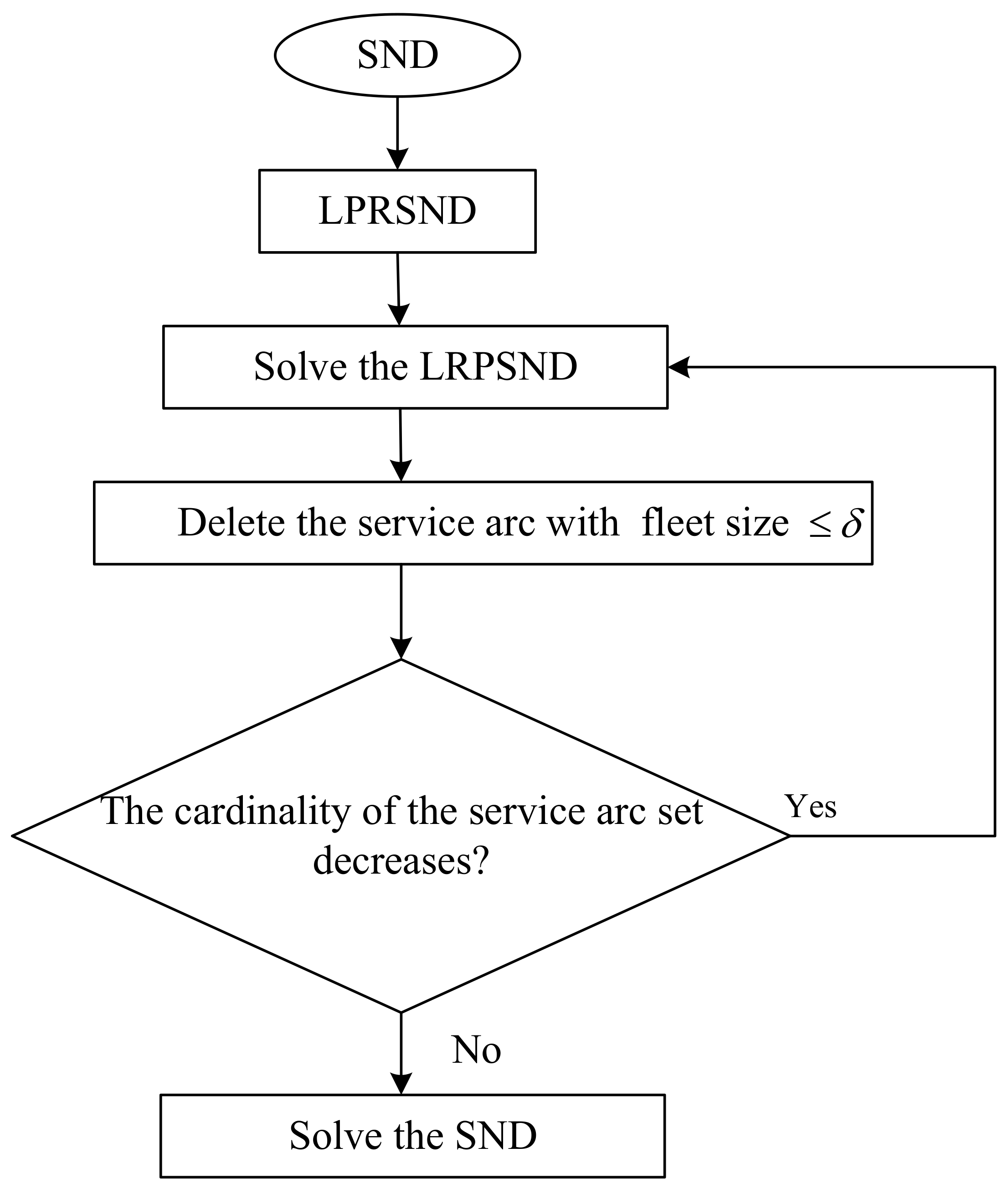
4. Solution Approach

We have to develop efficient algorithms for large-scale SND problems since they are NP-hard to solve [30]. In this section, we propose an iterative backbone algorithm to solve large-scale applications to obtain solutions.

First, we obtain the linear programming relaxation of the SND (LPRSND) problem. The formulation of LRPSND is shown as follows:

Decision Variables:

$$\begin{array}{cc}{x}_{ij}^f\in {\mathbb{R}}_{+}& \mathrm{Fleet} \mathrm{size} \mathrm{of} \mathrm{vehicle} \mathrm{model} f \mathrm{on} \mathrm{arc} (i,j),\hfill \\ y_{ij}^k\in {\mathbb{R}}_{+}& \mathrm{The} \mathrm{flow} \mathrm{volume} \mathrm{of} \mathrm{commodity} k \mathrm{on} \mathrm{arc} (i,j).\hfill \end{array}$$

Formulation:

$$\begin{array}{c}\hfill Minimize \sum _{f\in \mathcal{F}}\sum _{(i,j)\in {\mathcal{A}}^f}{c}_{ij}^f{x}_{ij}^f\end{array}$$

subject to:

$$\sum _{j\in \mathcal{N}:(i,j)\in {\mathcal{A}}^f}{x}_{ij}^f-\sum _{j\in \mathcal{N}:(j,i)\in {\mathcal{A}}^f}{x}_{ji}^f=0\forall f\in \mathcal{F},\forall i\in \mathcal{N},$$

(6)

$$\sum _{(i,j)\in {\mathcal{A}}^k:i=k.o}{y}_{ij}^k=d_k\forall k\in \mathcal{K},$$

(7)

$$\sum _{(i,j)\in {\mathcal{A}}^k:j=k.d}{y}_{ij}^k=d_k\forall k\in \mathcal{K},$$

(8)

$$\sum _{(i,j)\in {\mathcal{A}}^k}{y}_{ij}^k=\sum _{(j,i)\in {\mathcal{A}}^k}{y}_{ji}^k\forall k\in \mathcal{K},\forall j\in \mathcal{N}:j\ne k.o,j\ne k.d,$$

(9)

$$\sum _{f\in \mathcal{F}}{x}_{ij}^f{u}^f-\sum _{k\in \mathcal{K}}{y}_{ij}^k\ge 0\forall (i,j)\in {\mathcal{A}}_s$$

(10)

Figure 3 illustrates the working mechanism of the algorithm with a flow chart. First, we set a threshold $\delta$ and solve the LPRSND. Then, we check the fleet size on the service arc in the optimal solution of the LPRSND. We drop the service arcs with fleet size less than $\delta$ and check whether the cardinality of the service arc set is decreased or not. If the cardinality decreases, we solve LPRSND in the next iteration. Every iteration after solving LRPSND, a service arc with a fleet size less than $\delta$ will be deleted, and the network scale becomes smaller and leaves a backbone. Then, we solve the original SND over the backbone network to obtain the optimal solution. We set $\delta$ to a tiny non-negative real number, and in this way, we can obtain the backbone.

5. Computational Study

This section reports the computational performance of the iterative backbone algorithm. The algorithm was implemented in Python, using Gurobi v9.1.2 as the IP and LP solver. All experiments were performed using a PC with a 2.9 GHz processor and 256 GB RAM running under a Windows 10 operating system.

5.1. The Settings of the Test Instances

We generated 24 instances with simulated data based on practical situations, which included two types of simulated test instances: middle-scale and large-scale ones. The middle-scale instances included 10–18 terminals and 6–10 time periods, whereas the large-scale instances included 20–30 terminals and 10 time periods. The large-scale instances could reflect the peak level of a practical express service system. We included all possible service arcs and o-d commodities between different terminals. The distance and traveling cost between two terminals were generated from practical situations. Each instance was characterized by its numbers of terminals, periods, arcs, and o-d commodities. The dimensionality is shown in

Table 1. Dimensionality of the middle-scale instances.

Instances	Terminals	Periods	Service Arcs	Waiting Arcs	Rotation Arcs	O-D Commodities
1	10	6	540	60	10	90
2	10	7	630	70	10	90
3	10	8	720	80	10	90
4	10	9	810	90	10	90
5	10	10	900	100	10	90
6	11	10	1100	110	11	110
7	12	10	1320	120	12	132
8	13	10	1560	130	13	156
9	14	10	1820	140	14	182
10	15	10	2100	150	15	210
11	16	10	2400	160	16	240
12	17	10	2720	170	17	272
13	18	10	3060	180	18	306

and

Table 2. Dimensionality of the large-scale instances.

Instances	Terminals	Periods	Service Arcs	Waiting Arcs	Rotation Arcs	O-D Commodities
1	20	10	3800	200	20	380
2	21	10	4200	210	21	420
3	22	10	4620	220	22	462
4	23	10	5060	230	23	506
5	24	10	5520	240	24	552
6	25	10	6000	250	25	600
7	26	10	6500	260	26	650
8	27	10	7020	270	27	702
9	28	10	7560	280	28	756
10	29	10	8120	290	29	812
11	30	10	8700	300	30	870

.

MIP gap denotes the relatively mixed integer programming (MIP) gap between the objective value of the best integer solution and the linear programming relaxation solution. For middle-scale instances, we set the limit as 300 s and the MIP gap was 1%, and if the solution reached any limitation, the algorithm stopped. We set the time limit as 3600 s and 5% as the MIP gap for large-scale instances. The dimensionality of middle-scale and large-scale instances are shown in Table 1 and Table 2. We generated 13 middle-scale instances and 11 large-scale instances in total.

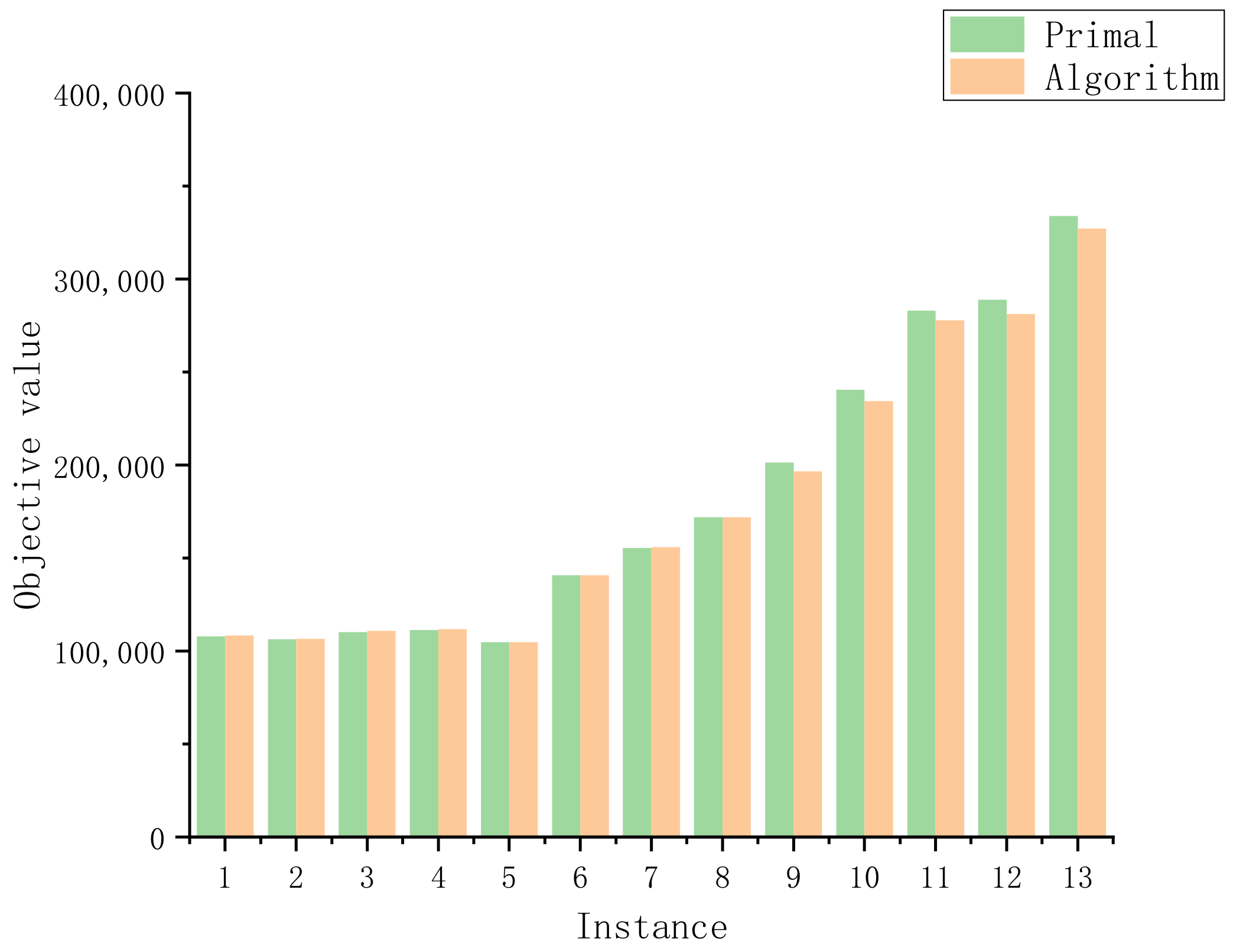
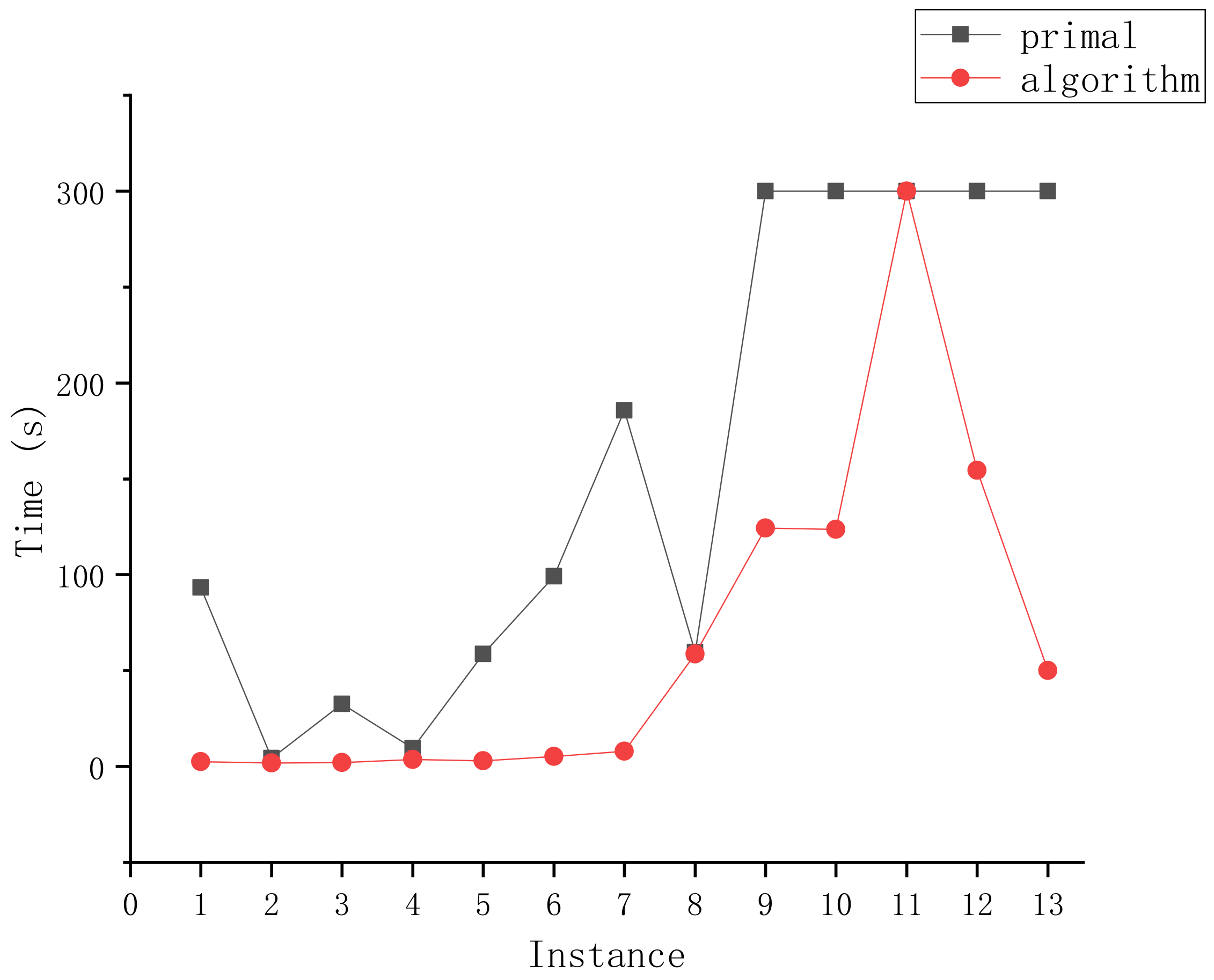
5.2. Numerical Results for Middle-Scale Instances

Table 3. Performancecomparisons over middle-scale instances. Maximum computational time was 300 s.

Instances	Primal Solution			Algorithm Solution
	Objective Value	Time (s)	MipGap	Objective Value	Time (s)	MipGap
1	108,026	93.364	0.659%	108,388	2.466	0.584%
2	106,311	4.387	0.971%	106,471	1.912	0.672%
3	110,258	32.725	0.770%	110,838	2.113	0.911%
4	111,310	9.489	0.849%	111,675	3.723	0.720%
5	104,650	58.595	0.996%	104,707	2.955	0.546%
6	140,672	99.172	0.929%	140,835	5.209	0.655%
7	155,432	185.72	0.819%	155,909	7.931	0.658%
8	171,934	59.611	0.431%	171,934	58.613	0.431%
9	201,334	300	3.488%	196,515	124.316	0.501%
10	240,476	300	3.479%	234,385	123.697	0.242%
11	282,930	300	3.480%	277,861	300	1.18%
12	288,994	300	4.005%	281,203	154.366	0.60%
13	333,992	300	3.487%	327,104	49.997	0.97%

reports the computational results with respect to middle-scale instances. The three columns related to primal SND formulation give the objective values, computational time in seconds, and MipGap of each instance solved directly by Gurobi. The next three columns were results obtained by the proposed algorithm. The results indicate that the proposed algorithm can efficiently and effectively solve middle-scale instances. The numerical results confirm the efficiency of the proposed algorithm: the computational time is significantly reduced compared to that of solving instances directly by Gurobi.

We show the objective value comparison in the middle-scale instances in Figure 4.

The objective values of the iterative backbone algorithm outperformed those of the primal solution with the growth of instance scale. As the scale increased, the objective value of the proposed algorithm became more prominent, and the maximum difference between two objective values reached 2.33%. Figure 5 compares the running time required by the primal formulation and our proposed algorithm. The time required by the iterative backbone algorithm is significantly less than that of the primal algorithm. In instances 9–13 of middle scale instances, the primal formulation did not achieve the required MIP gap within 300 s. These results confirmed that the effectiveness of the proposed algorithm is significantly better than that of solving SND directly by Gurobi.

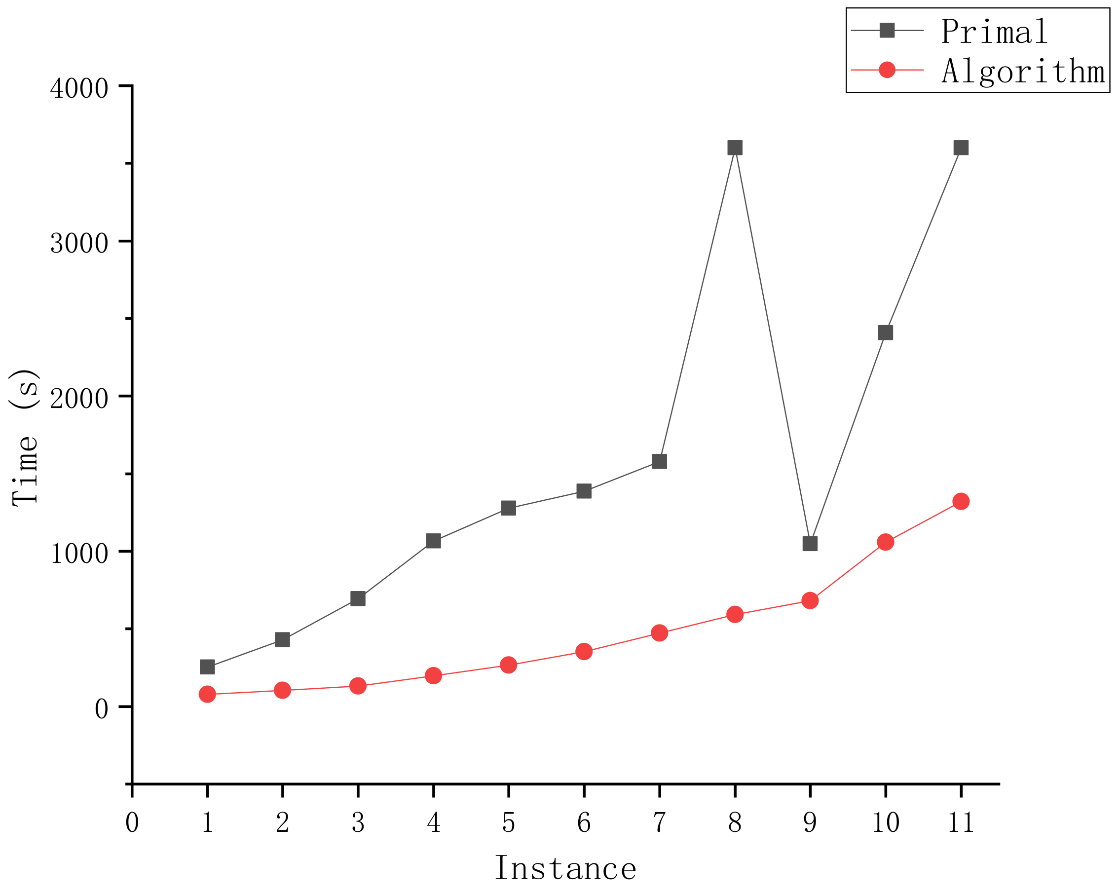
5.3. Numerical Results for Large-Scale Instances

The computational results for large-scale instances are shown in

Table 4. Performance comparisons over large-scale instances. Maximum computational time was 3600 s.

Instances	Primal Formulation			Algorithm Solution
	Objective Value	Time (s)	MipGap	Objective Value	Time (s)	MipGap
1	429,374	253.38	3.632%	427,374	79.103	3.632%
2	473,947	429.229	3.599%	473,947	104.698	3.599%
3	527,062	695.665	3.360%	527,062	131.458	3.360%
4	564,208	1065.901	3.805%	564,208	198.915	3.805%
5	626,500	1276.453	3.706%	626,500	265.52	3.706%
6	683,395	1387.908	3.471%	683,605	354.024	3.501%
7	748,470	1578.352	3.367%	748,370	473.046	3.354%
8	N.A.	3600	N.A.	782,448	591.897	3.678%
9	828,434	1052.945	3.675%	828,434	682.609	3.675%
10	913,316	2409.463	3.676%	913,316	1057.459	3.676%
11	N.A.	3600	N.A.	968,393	1321.356	3.447%

.

The primal formulation often takes two to five times as long as our algorithm. Moreover, as the scale increases, the primal formulation can not obtain a feasible integer solution within the time limit. However, the proposed iterative backbone algorithm can efficiently solve all instances. We show the objective values in Figure 6. It can be seen in the figure that instances 8 and 11 could not obtain one integer solution within the time limit, whereas the algorithm proposed by us obtained the solutions in 591 and 1321 s. The objective value of the primal solution was better only in instance 6.

Figure 7 compares the running time required to obtain the objective. The running times of the proposed algorithm are significantly shorter than those of solving SND directly, which confirms the proposed algorithm’s effectiveness in improving efficiency and finding high-quality solutions for large-scale applications.

6. Conclusions

In this work, we addressed the service network design problem for the real applications of express service providers and presented a mixed-integer optimization model. The mode integrates commodity flow, vehicle dispatching, and fleet sizing. Since the SND problem is NP-hard and there is a lack of efficient algorithms to solve large-scale applications, we presented an iterative backbone algorithm to solve it. The computational study indicates that the algorithm speeds up the computational process and outperforms the primal formulation solved by the state-of-the-art MIP solver Gurobi. The solution quality is also better than that of the primal solution in most cases.

With the continuous growth of transportation demand, service network design algorithms will become increasingly important. Although this algorithm has high efficiency, it essentially belongs to the class of heuristic algorithms. Theoretical proofs cannot guarantee the solution quality. Therefore, the future study will focus on developing efficient exact algorithms to solve the proposed formulations, i.e., a branch-and-price framework. Since the branching process makes intractable progress, we will resort to reinforcement learning approaches to accelerate the branch and bound process to enhance the branch-and-price algorithm. Another research direction is to find valid inequalities to strengthen the formulation. These inequalities could reduce the feasible region so that one can apply the solver to find the optimal solution faster.

References

1. UPS. 2021 Annual Report on Form 10-k; Technical Report; UPS: Atlanta, GA, USA, 2021. [Google Scholar]
2. FedEx. 2021 Annual Report: Moving the World Forward; Technical Report; FedEx: Memphis, TN, USA, 2021. [Google Scholar]
3. Crainic, T.G.; Gendreau, M.; Gendron, B. Service network design. In Network Design with Applications to Transportation and Logistics; Springer: Cham, Switzerland, 2021; pp. 347–382. [Google Scholar]
4. Goodarzian, F.; Hosseini-Nasab, H. Applying a fuzzy multi-objective model for a production–distribution network design problem by using a novel self-adoptive evolutionary algorithm. Int. J. Syst. Sci. Oper. Logist. 2021, 8, 1–22. [Google Scholar] [CrossRef]
5. Zhang, X.; Liu, X. A two-stage robust model for express service network design with surging demand. Eur. J. Oper. Res. 2022, 299, 154–167. [Google Scholar] [CrossRef]
6. Magnanti, T.L.; Wong, R.T. Network design and transportation planning: Models and algorithms. Transp. Sci. 1984, 18, 1–55. [Google Scholar] [CrossRef] [Green Version]
7. Pedersen, M.B.; Crainic, T.G.; Madsen, O.B. Models and tabu search metaheuristics for service network design with asset-balance requirements. Transp. Sci. 2009, 43, 158–177. [Google Scholar] [CrossRef]
8. Hewitt, M.; Lehuédé, F. The Service Network Scheduling Problem. 2022. hal-03598983v2f.
9. Hewitt, M. The Flexible Scheduled Service Network Design Problem. Transp. Sci. 2022. [Google Scholar] [CrossRef]
10. Dayarian, I.; Rocco, A.; Erera, A.; Savelsbergh, M. Operations design for high-velocity intra-city package service. Transp. Res. Part B Methodol. 2022, 161, 150–168. [Google Scholar] [CrossRef]
11. Bilegan, I.C.; Crainic, T.G.; Wang, Y. Scheduled service network design with revenue management considerations and an intermodal barge transportation illustration. Eur. J. Oper. Res. 2022, 300, 164–177. [Google Scholar] [CrossRef]
12. Balakrishnan, A.; Magnanti, T.L.; Mirchandani, P.; Wong, R.T. Network Design with Routing Requirements. In Network Design with Applications to Transportation and Logistics; Springer: Cham, Switzerland, 2021; pp. 209–253. [Google Scholar]
13. Crainic, T.G.; Gendron, B.; Kazemzadeh, M.R.A. A Taxonomy of Multilayer Network Design and a Survey of Transportation and Telecommunication Applications. Eur. J. Oper. Res. 2022, 303, 1–13. [Google Scholar] [CrossRef]
14. Farahani, R.Z.; Rezapour, S.; Drezner, T.; Fallah, S. Competitive supply chain network design: An overview of classifications, models, solution techniques and applications. Omega 2014, 45, 92–118. [Google Scholar] [CrossRef]
15. Zhang, X.; Zou, B.; Feng, Z.; Wang, Y.; Yan, W. A Review on Remanufacturing Reverse Logistics Network Design and Model Optimization. Processes 2021, 10, 84. [Google Scholar] [CrossRef]
16. Minoux, M. Networks synthesis and optimum network design problems: Models, solution methods and applications. Networks 1989, 19, 313–360. [Google Scholar] [CrossRef]
17. Crainic, T.G.; Rousseau, J.M. Multicommodity, multimode freight transportation: A general modeling and algorithmic framework for the service network design problem. Transp. Res. Part B Methodol. 1986, 20, 225–242. [Google Scholar] [CrossRef]
18. Kim, D.; Barnhart, C.; Ware, K.; Reinhardt, G. Multimodal express package delivery: A service network design application. Transp. Sci. 1999, 33, 391–407. [Google Scholar] [CrossRef]
19. Lai, M.F.; Lo, H.K. Ferry service network design: Optimal fleet size, routing, and scheduling. Transp. Res. Part A Policy Pract. 2004, 38, 305–328. [Google Scholar] [CrossRef]
20. Zhu, E.; Crainic, T.G.; Gendreau, M. Scheduled service network design for freight rail transportation. Oper. Res. 2014, 62, 383–400. [Google Scholar] [CrossRef] [Green Version]
21. Caramia, M.; Guerriero, F. A heuristic approach to long-haul freight transportation with multiple objective functions. Omega 2009, 37, 600–614. [Google Scholar] [CrossRef]
22. Scherr, Y.O.; Neumann-Saavedra, B.A.; Hewitt, M.; Mattfeld, D.C. Service network design for same day delivery with mixed autonomous fleets. Transp. Res. Procedia 2018, 30, 23–32. [Google Scholar] [CrossRef]
23. Scherr, Y.O.; Saavedra, B.A.N.; Hewitt, M.; Mattfeld, D.C. Service network design with mixed autonomous fleets. Transp. Res. Part E Logist. Transp. Rev. 2019, 124, 40–55. [Google Scholar] [CrossRef]
24. Barnhart, C.; Schneur, R.R. Air network design for express shipment service. Oper. Res. 1996, 44, 852–863. [Google Scholar] [CrossRef]
25. Yu, S.; Yang, Z.; Yu, B. Air express network design based on express path choices–Chinese case study. J. Air Transp. Manag. 2017, 61, 73–80. [Google Scholar] [CrossRef]
26. Demir, E.; Burgholzer, W.; Hrušovský, M.; Arıkan, E.; Jammernegg, W.; Van Woensel, T. A green intermodal service network design problem with travel time uncertainty. Transp. Res. Part B Methodol. 2016, 93, 789–807. [Google Scholar] [CrossRef]
27. Zhao, R.; Liu, W.; Zhang, F.; Koo, T.T.; Lodewijks, G. Passenger shuttle service network design in an airport. Transp. Transp. Dyn. 2022, 10, 1099–1125. [Google Scholar] [CrossRef]
28. Lanza, G.; Crainic, T.G.; Rei, W.; Ricciardi, N. Scheduled service network design with quality targets and stochastic travel times. Eur. J. Oper. Res. 2021, 288, 30–46. [Google Scholar] [CrossRef]
29. Jiang, X.; Bai, R.; Atkin, J.; Kendall, G. A scheme for determining vehicle routes based on Arc-based service network design. INFOR Inf. Syst. Oper. Res. 2017, 55, 16–37. [Google Scholar] [CrossRef]
30. Li, X.; Ding, Y.; Pan, K.; Jiang, D.; Aneja, Y.P. Single-path service network design problem with resource constraints. Transp. Res. Part E Logist. Transp. Rev. 2020, 140, 101945. [Google Scholar] [CrossRef]
31. Ghamlouche, I.; Crainic, T.G.; Gendreau, M. Cycle-based neighbourhoods for fixed-charge capacitated multicommodity network design. Oper. Res. 2003, 51, 655–667. [Google Scholar] [CrossRef] [Green Version]
32. Andersen, J.; Crainic, T.G.; Christiansen, M. Service network design with management and coordination of multiple fleets. Eur. J. Oper. Res. 2009, 193, 377–389. [Google Scholar] [CrossRef]
33. Andersen, J.; Christiansen, M.; Crainic, T.G.; Grønhaug, R. Branch and price for service network design with asset management constraints. Transp. Sci. 2011, 45, 33–49. [Google Scholar] [CrossRef]
34. Crainic, T.G.; Hewitt, M.; Toulouse, M.; Vu, D.M. Service network design with resource constraints. Transp. Sci. 2016, 50, 1380–1393. [Google Scholar] [CrossRef] [Green Version]
35. Boland, N.; Hewitt, M.; Marshall, L.; Savelsbergh, M. The continuous-time service network design problem. Oper. Res. 2017, 65, 1303–1321. [Google Scholar] [CrossRef] [Green Version]
36. Chiou, S.W. Bilevel programming for the continuous transport network design problem. Transp. Res. Part B Methodol. 2005, 39, 361–383. [Google Scholar] [CrossRef]
37. Di, Z.; Yang, L.; Qi, J.; Gao, Z. Transportation network design for maximizing flow-based accessibility. Transp. Res. Part B Methodol. 2018, 110, 209–238. [Google Scholar] [CrossRef]
38. Haider Bangyal, W.; Hameed, A.; Ahmad, J.; Nisar, K.; Haque, M.R.; Ibrahim, A.; Asri, A.; Rodrigues, J.J.; Khan, M.A.; BRawat, D.; et al. New modified controlled bat algorithm for numerical optimization problem. Comput. Mater. Contin. 2022, 70, 2241–2259. [Google Scholar] [CrossRef]
39. Bangyal, W.H.; Hameed, A.; Alosaimi, W.; Alyami, H. A new initialization approach in particle swarm optimization for global optimization problems. Comput. Intell. Neurosci. 2021, 2021, 6628889. [Google Scholar] [CrossRef] [PubMed]
40. Pervaiz, S.; Ul-Qayyum, Z.; Bangyal, W.H.; Gao, L.; Ahmad, J. A systematic literature review on particle swarm optimization techniques for medical diseases detection. Comput. Math. Methods Med. 2021, 2021, 5990999. [Google Scholar] [CrossRef]
41. Crainic, T.G.; Frangioni, A.; Gendron, B. Bundle-based relaxation methods for multicommodity capacitated fixed charge network design. Discret. Appl. Math. 2001, 112, 73–99. [Google Scholar] [CrossRef]
42. Li, X.; Wei, K.; Aneja, Y.P.; Tian, P. Design-balanced capacitated multicommodity network design with heterogeneous assets. Omega 2017, 67, 145–159. [Google Scholar] [CrossRef]
43. Li, X.; Wei, K.; Guo, Z.; Wang, W.; Aneja, Y.P. An exact approach for the service network design problem with heterogeneous resource constraints. Omega 2021, 102, 102376. [Google Scholar] [CrossRef]
44. Chu, J.C. Mixed-integer programming model and branch-and-price-and-cut algorithm for urban bus network design and timetabling. Transp. Res. Part B Methodol. 2018, 108, 188–216. [Google Scholar] [CrossRef]
Figure 1. Express service network.
Processes 10 01373 g001
Figure 2. Time-space network.
Processes 10 01373 g002
Figure 3. Flow chart of the algorithm.
Processes 10 01373 g003
Figure 4. Objective values for middle-scale instances.
Processes 10 01373 g004
Figure 5. Running time for middle-scale instances.
Processes 10 01373 g005
Figure 6. Objective values for large-scale instances.
Processes 10 01373 g006
Figure 7. Running time for large-scale instances.
Processes 10 01373 g007