Development of a Hydrokinetic Turbine Backwater Prediction Model for Inland Flow through Validated CFD Models

Abstract

Hydrokinetic turbine deployment in inland water reticulation systems such as irrigation canals has potential for future renewable energy development. Although research and development analysing the hydrodynamic effects of these turbines in tidal applications has been carried out, inland canal system applications with spatial constraints leading to possible blockage and backwater effects resulting from turbine deployment have not been considered. Some attempts have been made to develop backwater models, but these were site-specific and performed under constant operational conditions. Therefore, the aim of this work was to develop a generic and simplified method for calculating the backwater effect of HK turbines in inland systems. An analytical backwater approximation based on assumptions of performance metrics and inflow conditions was tested using validated computational fluid dynamics (CFD) models. For detailed prediction of the turbine effect on the flow field, CFD models based on Reynolds-averaged Navier–Stokes equations with Reynolds stress closure models were employed. Additionally, a multiphase model was validated through experimental results to capture the water surface profile and backwater effect with reasonable accuracy. The developed analytical backwater model showed good correlation with the experimental results. The model’s energy-based approach provides a simplified tool that is easily incorporated into simple backwater approximations, while also allowing the inclusion of retaining structures as additional blockages. The model utilizes only the flow velocity and the thrust coefficient, providing a useful tool for first-order analysis of the backwater from the deployment of inland turbine systems.

1. Introduction

Research and development of hydrokinetic (HK) devices in canal systems is increasing in popularity due to increasing electricity costs and the drive towards finding renewable energy sources with unconventional applications [1,2,3]. Although most development has focussed on tidal applications, multiple opportunities exist for the deployment of HK systems within inland water infrastructure (e.g., canal systems) [1]. However, the placement of such a device can have significant water level and hydrodynamic energy loss effects [4].

Prediction of the hydrodynamic effects of hydrokinetic turbines in canal systems remains an important pre-development objective. Due to the nature of canal design, these systems usually have flat slopes and subcritical flow regimes. Therefore, the analysis of backwater effects from blockages is critical for the prevention of flooding and water loss. This is especially important in array schemes where the cumulative effect of multiple devices can exceed the top of the channel and cause it to overtop.

Generally, backwater calculations utilize a blockage size (e.g., typical backwards-facing step, weir or pier shape) or energy loss function (quantified energy losses) to predict the backwater effect. Due to the novelty of HK energy, a streamlined procedure for determining the backwater effect has not yet been determined. This may be attributed to the variability of turbine types, operational conditions, and efficiencies, all of which result in a different effective blockage.

Previous studies have investigated the hydrodynamic effects of horizontal-axis hydrokinetic turbines (HAHTs) both experimentally (e.g., in canals [5], investigating boundary layers [6] and varying Reynolds numbers [7]) and computationally (e.g., both CFD applications in [4,8]). However, most of the studies are performed under constant operational conditions, and are site-specific (e.g., three-bladed [9] and two-bladed [9,10] turbines under optimal conditions). Some attempts have been made in the past to develop backwater models using roughness values [4] or analytical relationships [11], but the lack of experimental results over a range of turbine designs and operational conditions has resulted in site-specific models. Additionally, use of the models without in-depth knowledge of input variables limits their utility.

This study aimed to develop a simplified method for calculating the backwater effect of HK turbines in canal systems. An analytical approximation based on assumptions of performance metrics and inflow conditions was tested using validated computational fluid dynamics (CFD) models. These models allow a larger dataset and, thus, validation of the analytical approximation recommended.

2. Background

Placement of an HK device extracting energy in confined flow may affect water surfaces and water surface profiles. This is especially true in array schemes, and must be considered to ensure that the clearance between the rotor blades and the surface is sufficient. Myers and Bahaj [12] investigated a 1:30 scale HAHT model (rotor diameter, d_T = 0.4 m), and observed a clear difference in the water surface once energy was extracted. Water depths increased immediately upstream of the rotor and decreased downstream for about 2 d_T. Details of the water surface profiles can be seen in Figure 1. The results observed a standing wave 7–8 d_T downstream (it should be noted that this was for the high-freestream-velocity case).

Prediction of such occurrences requires understanding of the specific energy and flow regime (Froude number) to predict flow behaviour after HK deployment; here, a Froude number based on turbine diameter ($F{r}_D=\frac{U}{\sqrt{g{d}_t}}$, where U is the mean velocity and d_t is the turbine diameter) may be more useful, which has also been found to govern the free-surface effects [13].

The flow effects observed can be explained using the specific energy of the flow section, which is a function of water depth and velocity. When ignoring friction losses (e.g., from the channel sides and bed), the specific energy may be defined as follows:

$$E=y+\frac{\alpha Q^2}{2g{A}^2}$$

(1)

where y is the water depth, α is the energy coefficient, Q is the volumetric flow rate, A is the cross-sectional area, and g is the gravitational acceleration. The energy coefficient can then be defined as follows:

$$\propto =\frac{\sum u^3\Delta A}{U^{3}A}$$

(2)

where A is the total flow area and u is the velocity measured within an elemental area, $\Delta A$. The flow regime (sub- or supercritical) and, thus, the Froude number of the flow govern the behaviour of the flow [14].

A parameter of specific interest is the critical depth of the channel in which the turbine is placed. When the water surface decreases to critical or subcritical depth, flow phenomena such as hydraulic jumps may form downstream to allow recovery to normal flow depth.

Simplification of crucial free-surface parameters in inland HK installations can be summarized by two fundamental effects:

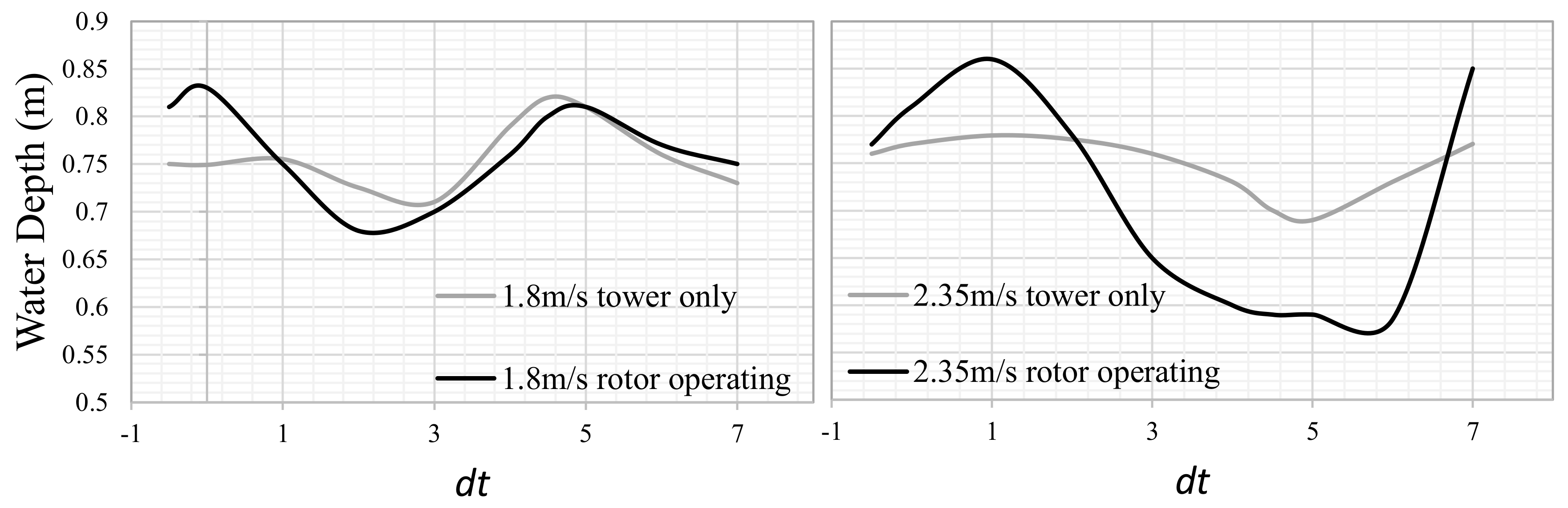
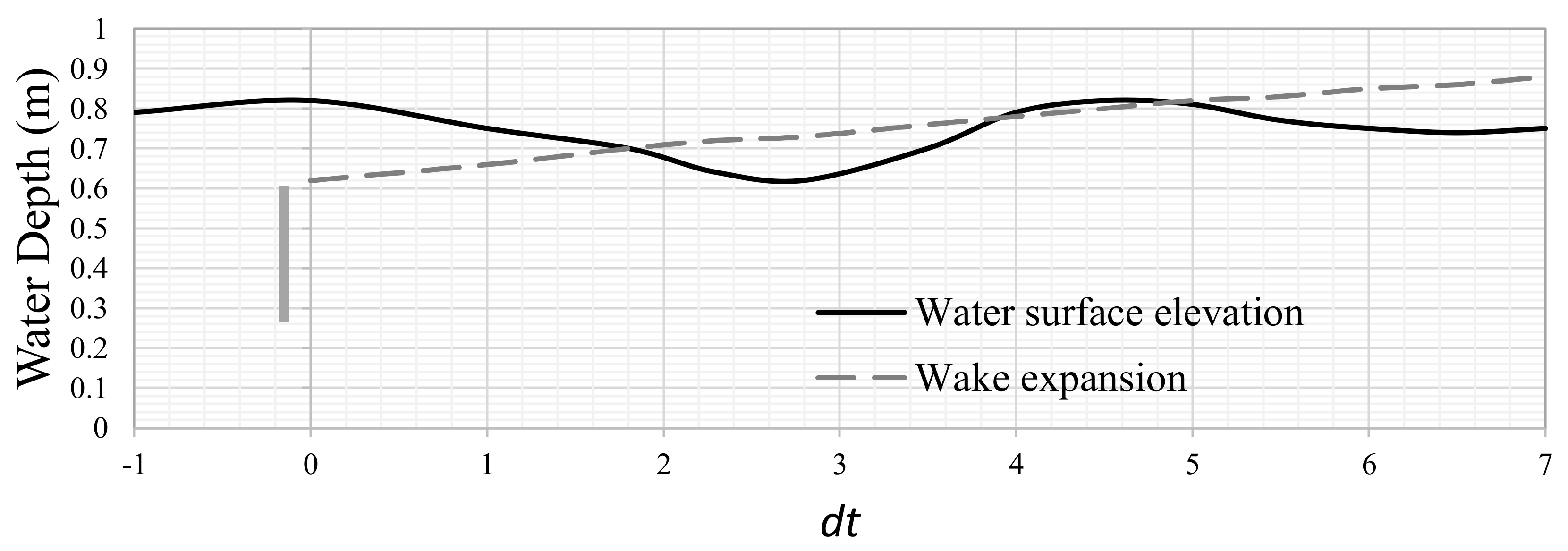
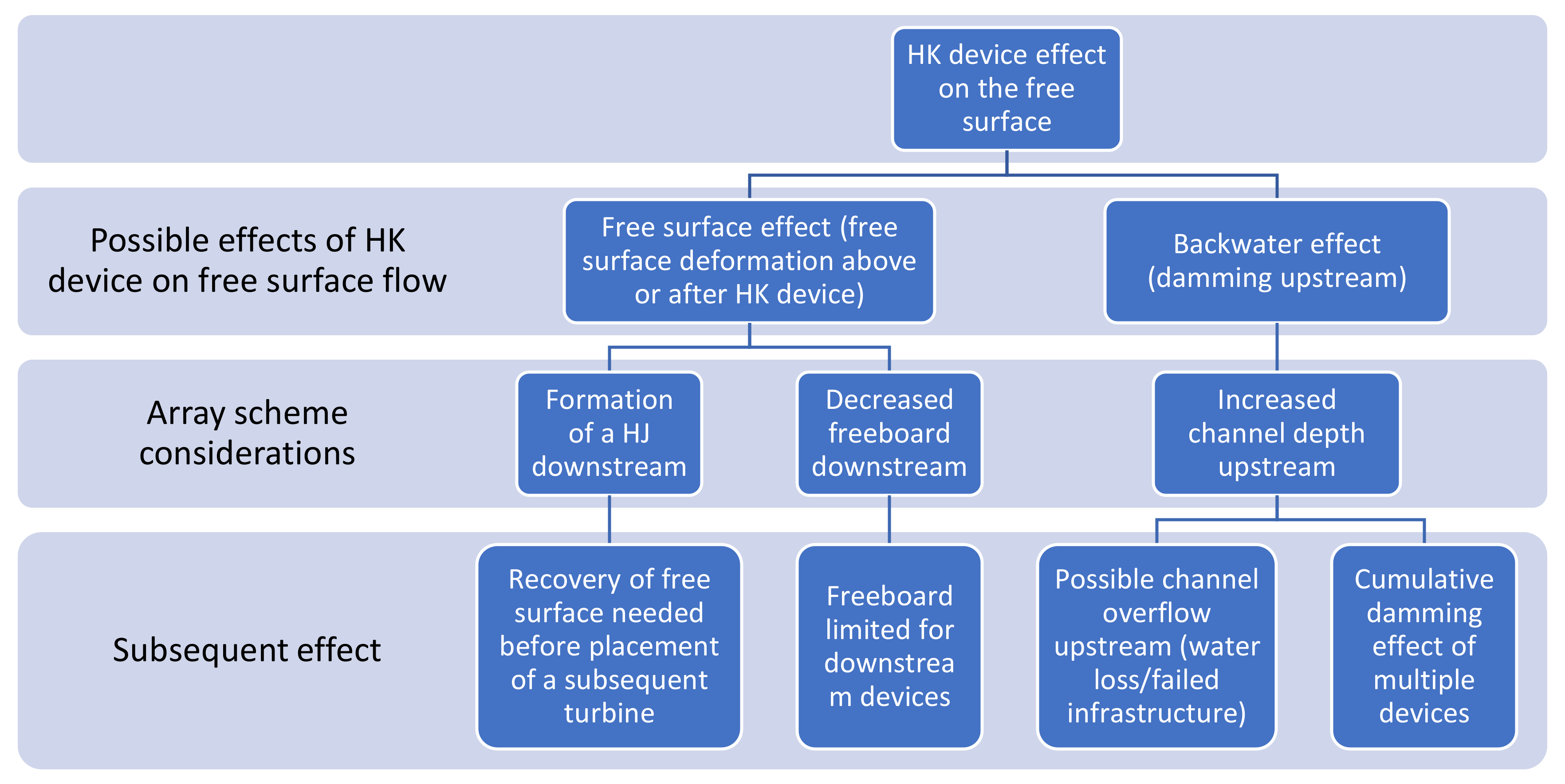
• Free-surface effects in the form of a possible standing wave formed, or decreased water surface above the turbine (due to decreasing pressure).
• Potential backwater effects caused (e.g., damming upstream).

2.1. Free-Surface Effects of HK Turbines

Free-surface effects are a critical aspect in riverine and tidal turbine array design, as the standing wave formed downstream of the turbine affects additional downstream turbines. Previous studies have concluded that the depth of the downstream water surface is strongly dependant on the Fr_D. Additionally, the blockage ratio also affects this free-surface change, albeit not as strongly as Fr_D [13]_.

Myers and Bahaj [12] found that when imposing the typical wake expansion on the water surface, this coincided with the increased elevation observed 4–5 d_t downstream of the turbine rotor (as shown in Figure 2). In addition, due to the wake expansion coincident with the free surface, cumulative turbine placement at intervals smaller than the recovery length may cause the flow to approach critical depth, causing severe undulations in the water surface profiles (WSPs). Turbine operation and efficiency may also vary due to decreasing fluid velocity over the blades during operation. Accurate quantification of the WSPs around an array may be a challenge due to the multiple effects of turbulence, wake mixing, and superposition of WSP effects [12].

The presence of a support structure (tower/stanchion) also strongly affects the free-surface effect [12] (Figure 1). The same experiment also indicated the strong possibility of the formation of a hydraulic jump downstream of the turbine when flow is forced to a supercritical level due to the presence of the turbine and support structure.

Free-surface effects may be more pronounced for shallow turbines compared to turbines installed well below the free surface. It is also important to consider possible cross-sectional changes in the infrastructure where the turbine is placed, as this may alter/dampen/exaggerate these effects. Specified clearance coefficients have been investigated to limit the severity of decreased depths downstream of the turbine, or possible exposure of the turbine. Birjandi [15] proposed a clearance coefficient, C_h, defined as follows:

$$C_h=\frac{H}{L}$$

(3)

where H is the turbine submergence depth (i.e., the height between the top of the turbine and the water surface) and L is the rotor diameter. The recommended clearance coefficients for commercially available turbines can be seen in

Table 1. Clearance coefficients for commercial HAHTs.

Turbine		Clearance Coefficient
Seaflow	2-Bladed, 300 kW	0.18–0.64
SeaGen	2-Bladed, 1.2 MW (2× 600 kW)	0.25–0.38
HS300	3-Bladed, 300 kW	0.75
AK-1000	3-Bladed, 1 MW	1.02

.

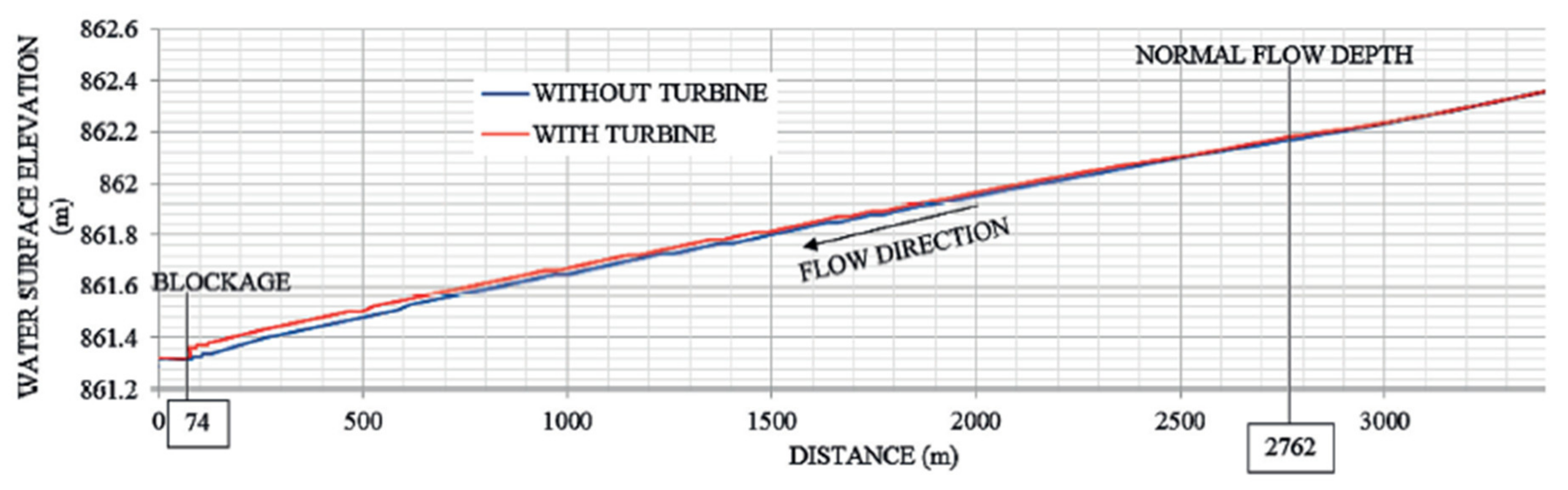
2.2. Backwater Effect

A turbine acts as a blockage in the channel and results in energy loss in inland flow infrastructure (where flow is constrained). When Fr << 1 and subcritical flow is prevalent, the backwater effect (damming upstream) may extend a large distance upstream as well as causing significant damming. This depends greatly on the blockage ratio, which is a function of the turbine swept area (A_T), channel flow area (A_o) ($BR\left(\%\right)=\raisebox{1ex}{$A_T$}\!\left/ \!\raisebox{-1ex}{$A_o$}\right.$), and additional constrictions [16], as well as the theoretical to actual efficiency [17].

In a study on a pilot HK installation in an irrigation canal, the backwater effect from the presence of the turbine extended up to 2.7 km upstream, due to the flat slope and subcritical flow present in the channel [1] (Figure 3). The clearance coefficient for this installation had not yet been defined. The specific turbine studied in that project contained grids upstream of the turbine, which trapped debris and caused a further increase in the backwater effect, to the point of channel overtopping. The blockage ratio for the installation was around 12.5%.

Additional to the blockage ratio, the Froude number (Fr) or Froude number based on turbine diameter (Fr_D) of the flow can influence the backwater effect. A previous study analysing this effect drew the following conclusions [13]:

• The upstream free-surface deformation increased with Fr_D.
• The location of maximum damming (i.e., the highest water level) moved closer to the turbine as Fr_D increased.

Previous studies have attempted to quantity the effective blockage of an HK device. Some have addressed this through the relationship of power extracted to total power dissipated by the devices [18], analytical relationships [11], and even enhanced Manning n-values quantifying the energy loss as a friction loss [4]. However, a simple formula quantifying the effective blockage for different turbine types and operational conditions is yet to be determined, and provides the motivation for this paper.

2.3. Backwater Calculations

The extraction of energy resulting from the HK device may also be analytically incorporated through the use of the momentum equation [19], where the power extraction term is added as a shear stress component (added to the effective shear stress caused by bed friction). Assuming gradually varied steady-state flow, the conservation of mass and momentum can be used to adjust the standard open-channel flow equation [20] with the addition of a term for artificial energy extraction [19]:

$$\left(1-\frac{Q^2}{h^3{b}^{2}g}\right)\frac{\partial h}{\partial x}=\frac{\partial h}{\partial x}\frac{Q^2}{g{h}^2{b}^3}-\frac{1}{\rho gbh}P {\tau }_{eff}$$

(4)

The effective shear (${\tau }_{eff}$) is defined as a combination of the bed shear (${\tau }_o$) and power extraction added as a shear term (${\tau }_{add}$):

$${\tau }_{eff}={\tau }_o+{\tau }_{add}=\rho \frac{g}{C^2}{U}^2+\frac{P_{x}R}{U}$$

(5)

where P is the wetted perimeter, C is the Chezy friction coefficient, and $P_x$ is the term added for power extraction, which may be more useful to express in terms of $P_A$ being the power extracted per unit area, as the flow passes through a plane where $P_x=\frac{P_A}{\Delta x}$ ($\Delta x$ being the change in distance). Such an effect can be seen graphically in Figure 4, where a 10% energy extraction term has been added.

A previous study [21] attempted to determine the backwater curve for instances when either the cross-section varied, the channel slope changed, or there was an obstacle in the channel and gradually varied flow was present. The model was based on the Bernoulli equation between two cross-sections. The energy loss between the cross-sections (related to distance) was termed the hydraulic loss, I, which can be calculated as follows:

$$I=\frac{n^2{U}^2}{R_H^{\frac{4}{3}}}$$

(6)

where n is the Manning roughness (s/m^1/3), R_h is the hydraulic radius of the channel (m), and U is the velocity of the water (m/s). The change in water levels (Δz) between two sections can then be determined between two significant cross-sections (e.g., 0 and 1) and calculated as shown in Equation (7), where $\alpha$ is the Coriolis coefficient and U₀ and U₁ are the average velocities over distance $\Delta L$:

$$\Delta z=\Delta L\left(\frac{I_0+I_1}{2}\right)+\frac{\alpha }{2g}\left(U_0^2-U_1^2\right)$$

(7)

Very few models have been developed to attempt to predict the backwater effect—mostly 1D analytical models [4,11]. Most studies have focussed on tidal arrays and using free-surface effects to determine the optimal number and placement of turbines [22,23]. Within tidal applications, free-surface effects are only of concern for tip clearance; therefore, these models have limitations within the application in steady inland channels where spatial constraints are of primary concern.

In a study by Kartezhnikova and Ravens [4], an increased Manning roughness coefficient was used on the channel section representing the hydrokinetic device. The n-value used was a function of the actual channel n-value, slope, water depth, device efficiency, blockage ratio, and device deployment density. This method can then be used to determine the hydraulic impact, as well as the impact of various device configurations.

The head loss associated with the channel friction ($h_{Lt})$ (used in the energy conservation equation) can be written as shown in Equation (8), as a function of cross-sectional area ($A_0$), channel hydraulic radius ($R_h$), discharge ($Q_n$), and the length over which the loss is applied (L).

$$h_{Lt}={\left(\frac{Q_n}{A_0{R}_h{}^{2/3}}\right)}^{2}L$$

(8)

Based on the assumption that the upstream and downstream velocity and pressure heads are equal, and assuming that the drag loss is negligible, the following equation for an enhanced bottom roughness ($n_t$) can be derived as a function of the total power dissipated ($h_p$), change in elevation ($\Delta z$), and channel Manning roughness coefficient ($n)$.

$$n_t=n{\left(1-\frac{h_p}{\Delta z}\right)}^{-1/2}$$

(9)

Lalander and Leijon [11] investigated the use of numerical and analytical models to determine the effects on upstream water levels in a river. The analytical models are dependent on the channel blockage (of the HK device) determining energy loss from the energy capture, as well as the energy losses in the wake. The numerical models are based on the same theory—that energy is removed, causing a power loss; thus, energy capture is a component of the total friction in the channel. The total head loss can be determined as the sum of the friction loss ($\Delta h_f$) and head loss caused by the turbine ($\Delta h_t$), and P_t is the total power of the turbine (W). The formulation of the stress term ${\tau }_f$ is shown in Equation (11), where f is equal to the Darcy–Weisbach coefficient (unitless) and U is the velocity of water (m/s).

$$\Delta h_{tot}=\Delta h_f+\Delta h_t=\frac{L}{\rho g{R}_h}\ast {\tau }_f+\frac{P_t}{\rho gQ}$$

(10)

$${\tau }_f=\frac{f\rho }{8}\ast U^2$$

(11)

It is also important to consider the blockage effect, which can increase the turbine power output [22,24].

2.4. Summary of Literature

When HK devices are placed in array schemes in inland channels/rivers, the cumulative effect and inter-effect of these devices should be well understood to avoid unfavourable free-surface effects. As shown in the organogram (Figure 5), the blockage resulting from the HK device (in typical subcritical, flat-sloped channels) may have multiple subsequent effects influencing downstream installations (within the array) as well as upstream flow conditions. Neglecting the free-surface effects in high-blockage cases may result in exposed downstream turbines (i.e., freeboard reduced), hydraulic jump formation (enforced critical flow), and upstream damming effects, and may also lead to potential blade-tip cavitation problems. Accurately quantifying the water surface effects is a challenge, and guidelines to avoid unfavourable conditions may be extremely useful.

For inland systems, the backwater effect and the calculation thereof are of primary concern. Existing models include multiple unknowns and assumptions of values required as inputs that may not be available to users. Development of a clear, simple, effective blockage approximation of an HK device that can be applied to typical backwater calculations is necessary.

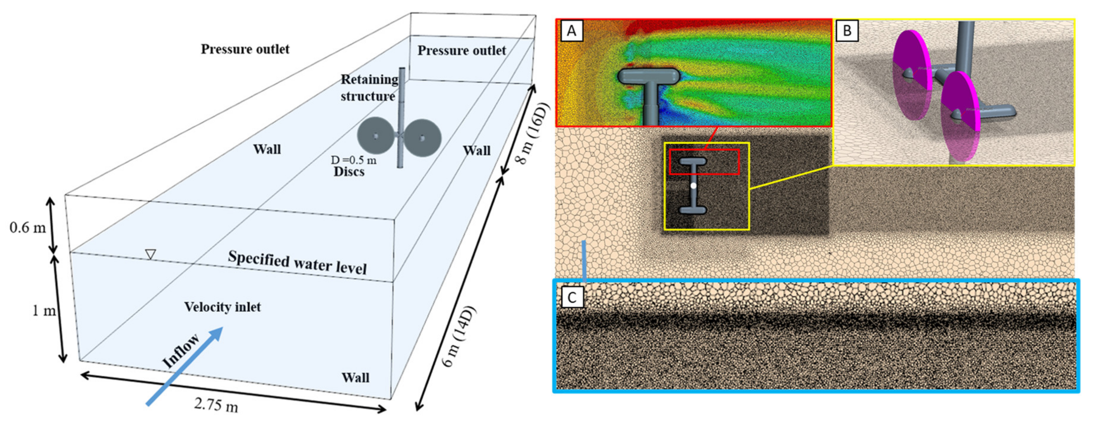
3. Validation of CFD Models

Comprehensive validation of a developed analytical model requires a dataset from a range of turbine styles under various operational conditions. Computational models offer an alternative to physical scale models to simulate the complex flow physics around HK devices. However, the importance of model validation through a physical model dataset should not be neglected. A number of studies have tested and validated modelling approaches for HK turbines [25,26].

Developments in tidal energy have led to multiple large-scale analyses of tidal turbine arrays, where simplified numerical models are used for array schemes [27,28,29,30]. With the ever-increasing availability and reliability of computational power, computational fluid dynamics (CFD) simulations are being used to model complex external effects and more accurately resolve fluid dynamic and wall effects [31]. Additionally, blade element momentum (BEM) theory is often used as a rotor modelling technique that also significantly reduces computational load [32].

CFD models may be used to resolve the effects of turbulence at the sub-grid-scale level, and are being used more often for first-order analysis or design. They have the potential to offer more comprehensive solutions and insights when their limitations are understood. Accurately representing turbulent flow in CFD is imperative due to its strong dependence on initial conditions, as well as the wide range of scales (eddies) present in the flow. Most often, statistical approaches based on the Reynolds-averaged Navier–Stokes (RANS) equations, with eddy viscosity models for turbulence closure, are used [33].

CFD models are valuable tools in flow-field analysis, especially at the sub-grid-scale level and for resolving turbulent length scales. When they are correctly applied and their limitations are understood, they offer useful insights and an alternative to laboratory testing. Correctly representing the turbulent flow, along with prescription of initial conditions, is important—especially due the wide range of scaled eddies present in the flow. Approaches based on the Reynolds-averaged Navier–Stokes (RANS) equations are most often used with various turbulence closure models incorporated, such as eddy viscosity models (k-Epsilon and SST k-ω).

A number of recent studies have used the BEM embedded in CFD method [8,34,35], which is also widely used in wind turbine array models, with good representation in terms of experimental results [36,37]. Various authors [38,39] have used this method to analyse the flow field of turbines arranged in arrays—specifically for tidal turbine optimization. A study analysing the accuracy of RANS approaches revealed good correlation with the experimental data found when using a Reynolds stress turbulence model (RSM) coupled with a BEM blade modelling technique (RSM-BEM) [40]. The study also highlights the importance of using an RSM rather than standard eddy viscosity models, due to the strong anisotropic flow in the wake.

3.1. CFD Models

Three different turbines (shown in

Table 2. Turbines modelled in CFD.

Turbine	Name	Blades	Diameter (m)	CFD Model
T1	RM1 [10]	2-Bladed NACA4415	0.5	Multiphase RSM-BEM model
T2	IFREMER [9]	3-Bladed NACA63418	0.7	Single-phase RSM-BEM model
T3	SHP [1]	3-Bladed custom blade	1	Single-phase RSM-FRG model

) were modelled using CFD and validated with experimental results (a variation of free-surface, wake, and performance measurements). The primary validation case used was the U.S. Department of Energy’s Reference Model 1 (RM1) dual-rotor axial flow turbine, which was modelled in the St. Anthony Falls Laboratory (SAFL) at the University of Minnesota [10]. Free-surface measurements allowed validation of the multiphase CFD model and free-surface deformation.

Additionally, two three-bladed turbine models with experimental results found in the literature [41] and tested on site [1] were modelled as specified in [40], for further measurements and validation of the backwater calculation methods. Where possible, BEM-VD (virtual disk) models were used to reduce the computational expense required. However, for the turbines which customized NACA profiles (Smart Hydropower turbine used in [1]) the full rotor geometry was modelled using a sliding mesh.

3.2. RM1 Model Validation

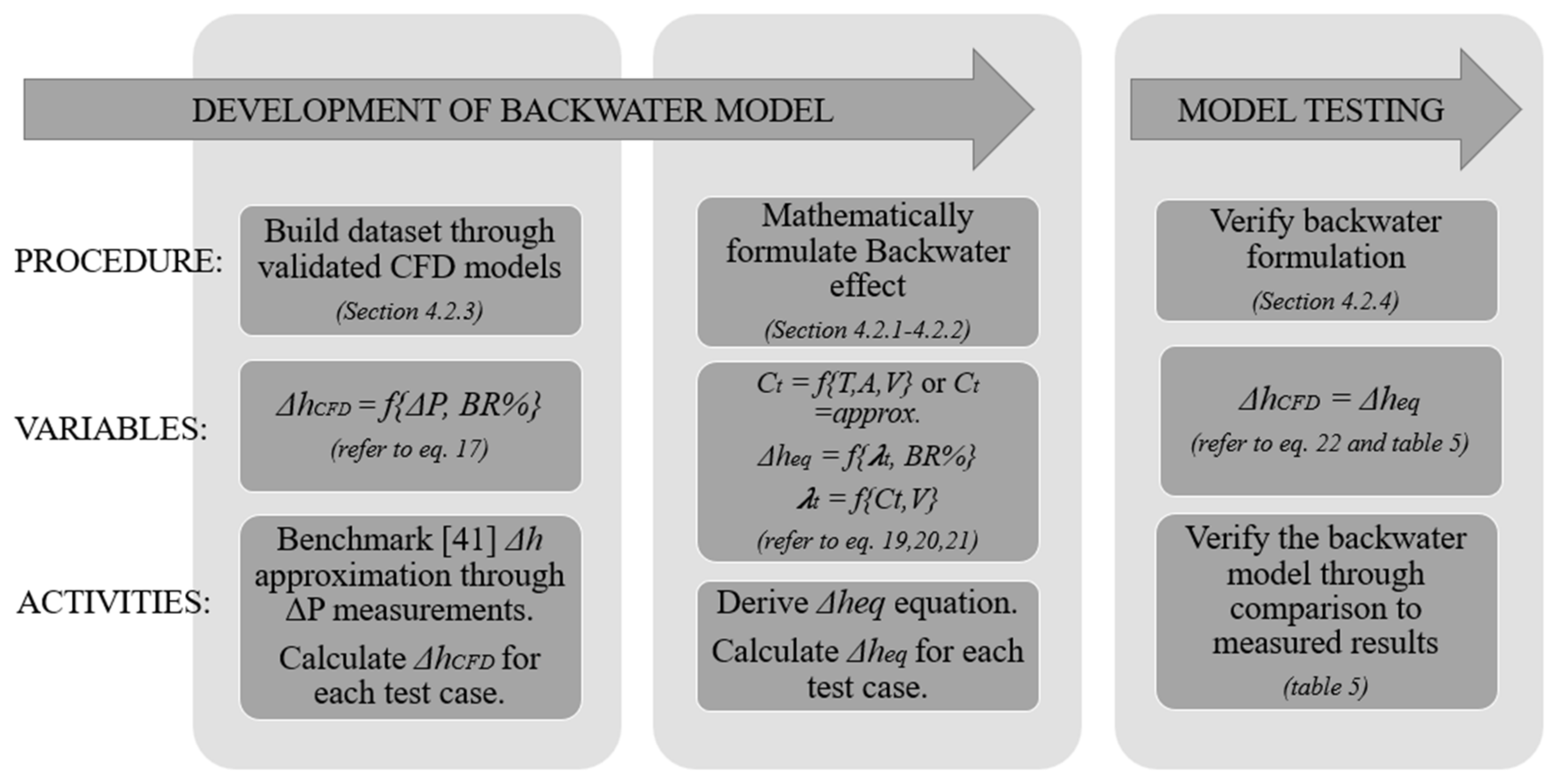
A 0.5 m diameter dual-rotor axial flow tidal turbine was investigated in a laboratory setup. The relevant details of the experiment can be seen in

Table 3. RM1 laboratory setup details [42].

Description	Variable
Rotor diameter	0.5 m
Blade profile	NACA 4415
Flow depth	1 m
Flow rate	2.425 m3/s
Tip speed ratios measured	1 to 9
Flow velocity (Uhub)	1.05 m/s
Turbulence intensity	5%
Froude number	0.28
Reynolds number (chord)	~3.0 × 105

, with additional details available in [42]. The experimental results [42] provide high-resolution wake measurements of the near- and far-wake flow field surrounding the turbine from −5 to 10 d_t. These were used previously to validate the CFD procedure for a single-phase analysis [40].

Although the velocity profiles and performance metrics were adequately modelled with both the single-phase and multiphase models, correct approximation of the backwater effect through the multiphase modelling required validation. For this, free-surface measurements were collected for the optimal operational case (TSR = 5.1, U = 1.05 m/s) of the RM1 experimental setup, at a resolution of 1 d_t (diameters) in the streamwise direction, and 0.4 d_t in the cross-stream direction. The measurement zone was −5 dt to 10 dt downstream. Elevation data were sampled at 50 Hz for 120 seconds at each location using a Massa ultrasonic range sensor, allowing for both time-averaged and fluctuating water surface elevation analysis and CFD validation.

Siemens STAR-CCM+ Commercial modelling software was used to simulate the turbines. The computational domain representing the RM1 laboratory model is shown in Figure 6. A wall-bounded model was used, extending from −14 d_t upstream to 16 d_t downstream of the axis of rotation. The specified inlet length allowed full flow development prior to reaching the turbine axis of rotation. The outlet length ensured that no effects from the downstream boundary condition affected the near-wake behaviour. Previous studies have found that around 15 d_t is usually adequate for the outlet boundary length [43,44].

A velocity inlet and downstream pressure outlet were specified as boundary conditions. The laboratory test turbulence and velocity values that were measured experimentally were specified at the inlet. Full development of the boundary layer on all surfaces (i.e., boundary walls, blades, and stanchion) was ensured through the specific turbulence model wall treatment and mesh resolution for each test case (details seen in [40]).

A virtual disk (VD) rotor modelling technique was used, and a BEM model was employed over the VD. This VD-BEM modelling approach has demonstrated good accuracy in the past, also significantly reducing computational costs [8,34,35,45,46]. A BEM tip-loss correction was incorporated using the Prandtl tip-loss correction method [47].

A Reynolds stress model (RSM) was used to allow more accuracy in prediction of possible flow anisotropy. The RS linear pressure strain two-layer (RS-LPS2) model [48,49] was found to model the near wake accurately, with a low y⁺ wall treatment on the turbine and turbine structure (y⁺ < 1).

Only transient simulations were performed, where unsteady terms were discretized using a 2nd-order implicit scheme. A time step ensuring Courant numbers of less than 1 over the domain was ensured as far as possible (some cells exceeded 1 at the blade tips, where smaller time steps did not change results and, therefore, larger Courant numbers were allowed to reduce computational time). The time steps were around 0.003 s for the BEM-CFD models. However, the time steps varied over each approach, depending on the results of the grid convergence index (GCI).

The computational domain (Figure 6) consisted of a polyhedral mesh with grid refinements in the free surface, near wake, far wake, and surrounding the turbine structure. In the past, results indicated the importance of fine grids to track the tip vortices when using simplified RANS models [31]. For grid refinement, an adapted GCI method [50] was used, due to the variance in grid sensitivity in the different regions. Separate regions’ mesh sizes were incrementally decreased, until no changes in turbine performance, free surface, or wake behaviour were observed. As depicted in Figure 6, the final mesh sizes were around 14 million cells.

The smallest cell sizes were specified at the near wake and free surface, where a 10 mm minimum size proved to be adequate. Refinement in the near-wake region is imperative for accurate development of the complex near-wake behaviour, where both separated and attached flow exist [51]. Gibson and Launder [52] investigated the pressure fluctuation effects of capturing the boundary layer surrounding the turbine, and noted the importance of an accurate capture of boundary layer formation. For the VD rotor modelling technique, a minimum of four cells over the blade thickness was ensured for all meshes, which is the recommended minimum when using the VD method. A mesh base size of 14 mm (2.8% d_t) proved adequate in the far-wake region.

The channel walls around the turbine were modelled as non-slip walls using a high-y+ wall treatment to ensure that the effects of the wall boundary layer were included in the simulation. A two-layer formulation may be applied to the linear pressure strain model (LPS2 model). All analyses used the two-layer formulation.

Simulation of the air–water interface (multiphase flow) may be approached in various ways. A multiphase analysis ensures a robust approach, but demands a higher computational load; therefore, a symmetry boundary condition is often used in a single-phase model [40].

Due to the necessity of free-surface measurements in this analysis, the free surface was modelled using a volume-of-fluid approach. This approach uses a 2nd-order discretization to compute a clear interface between the air and water. A volume-fraction variable is used to specify the spatial distribution of each phase. Cells with multiple phases are treated as mixtures, and the method is highly dependent on adequate mesh resolution. A high-resolution mesh (Figure 6C) was ensured on the free surface, with the final cell size determined through a GCI test focussed on a free-surface profile analysis.

Validation of the modelled wake and performance can be seen in [40]. Due to the importance of the backwater approximation, and correct modelling of the backwater effect caused by the turbine blockage, the free-surface measurements from a multiphase model were compared in this paper. Comparison of the experimental and CFD results can be seen in Figure 7. The results correlated well, with the computed free-surface behaviour fitting well with the experimental tests. The CFD results were recorded over one rotation and plotted as an envelope. The backwater effect was predicted well, with a maximum of 12 mm damming occurring upstream.

4. Methods

The primary objective of the development of a backwater model is to allow a usable model with only basic inputs required. Thus, a mathematical formulation based on existing models, basic hydrodynamic principles, and a set of recommended assumptions (where/if information is not yet available) was carried out. The workflow for the backwater model’s development can be seen in Figure 8, and is explained in the following subsections.

4.1. Assumptions and Exclusions

It is important to state the limitations of the model. Operational condition boundaries were set to within the typical canal operating conditions, where deployment of HK devices would be considered. Scenarios outside of these boundaries were not considered, as it was assumed that the use of such a model would not be necessary outside of these conditions (e.g., at supercritical flow conditions) [1,14,53].

The following limitations on flow conditions were set:

• Subcritical flow regime (Fr < 1);
• 5000 < Re < 1,500,000;
• Typical operational velocities of channels (0.8–2.8 m/s);
• Manning n-value around 0.016–0.023 s/m^1/3 (lined channel).

4.2. Mathematical Formulation

Energy losses in a channel are categorized and included with various approximations. For channel roughness, the friction losses can be accounted for by the Manning equation. Additionally, sudden losses due to channel features such as piers, bends, and drop structures have also been defined/estimated empirically, and can be included as form losses [14]. These are typically defined as eddy losses (h_e), included as an energy loss:

$$h_e=C_L\frac{V^2}{2g}$$

(12)

where C_L is the loss coefficient predefined for typical losses in a channel. The drop in water level due to a particular loss can be quantified/included by applying either the momentum or energy equation over a channel section, and the upstream and downstream sections (in which the energy loss exists). Additionally, an empirical approach may be used, where experimental results are used to determine an empirical relationship, such as that done by Yarnell in 1934 for bridge piers [54].

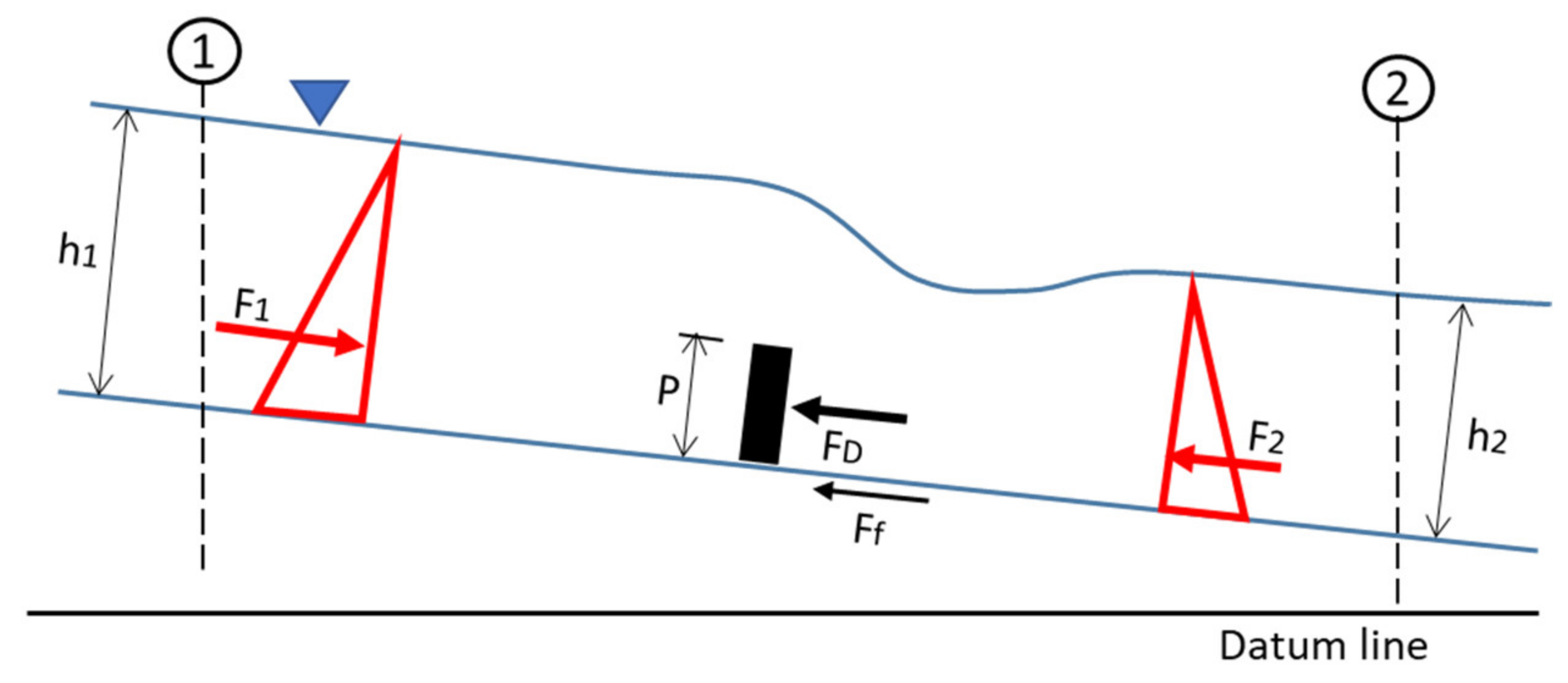
4.2.1. Approach 1: Momentum Approach

A possible approach often used to determine the effect of an object/structure on the free surface (backwater effect) is the momentum approach. Energy losses occur due to flow separation, vortex generation, friction, and turbulence—all associated with the changes in velocity due to the presence of the turbine. In some cases, the presence of the turbine may also result in the formation of a hydraulic jump on the water surface, resulting in additional energy losses. Applying the momentum approach avoids inclusion of these individual energy losses by considering the change in momentum between an upstream and downstream section. Additionally, if drag can be quantified, the momentum approach may be favourable.

The simple momentum formulation between two flow sections can be used with the resistance of the turbine represented as a drag coefficient, as shown in Figure 9 and Equation (13), where the change in momentum is quantified by the hydrostatic forces upstream (F₁) and downstream (F₂) of the device (water level change), as well as the friction from the channel bed and walls (F_f) and the force due to the turbine (F_D). This can then be rewritten to Equation (14), in terms of the drag force (F_D) due to the presence of the turbine.

$$F_1-F_2-F_D-F_f=\rho Q\left({\beta }_2{V}_2-{\beta }_1{V}_1\right)$$

(13)

$$F_D=\frac{1}{2}\rho gB{h}_1{}^2-\frac{1}{2}\rho gB{h}_2{}^2-\rho Q\left({\beta }_2{V}_2-{\beta }_1{V}_1\right)$$

(14)

The drag coefficient for the HK device can be rewritten, which allows the determination of $h_1$ (the upstream water level) through knowledge of the drag coefficient and downstream flow conditions. However, this requires knowledge of the downstream conditions, which is not always possible in feasibility studies in the design phase. An alternative conservative analysis would be to use the normal flow depth as the downstream value.

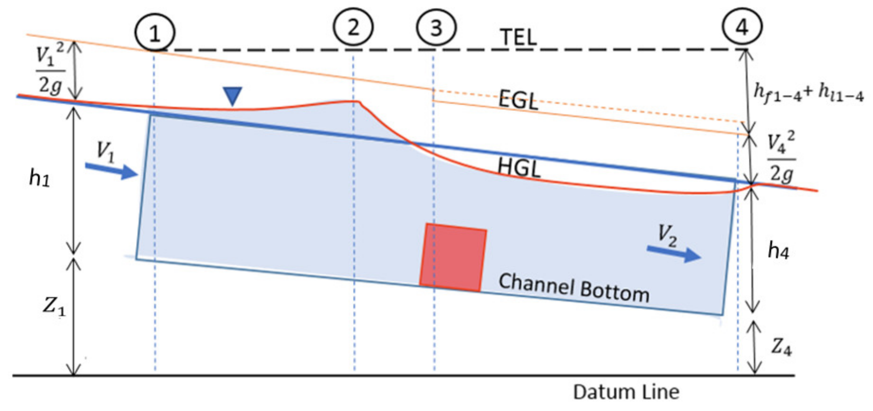
4.2.2. Approach 2: Energy Approach

The energy approach is more often used to determine backwater effects in typical open-channel flow scenarios. This is also a common approach in bridge pier modelling [14] when modelling the backwater effect of arch bridges [56], bridge piers, and even irregular structures such as wood jams [57].

The energy approach can be seen in Equation (15) and Figure 10. All energy losses between a point upstream and downstream of an HK device or blockage are quantified as terms that contribute to either the friction losses (h_f) or local losses (h_l).

$$\frac{V_1{}^2}{2g}+h_1+Z_1=\frac{V_4{}^2}{2g}+h_4+Z_4+\sum h_f{}_{1-4}+\sum h_l{}_{1-4}$$

(15)

All terms are defined in terms of velocity U), water depth (h), and distance from a datum (Z). The total energy (TEL), energy grade line (EGL), and water level/hydraulic grade line (HGL) are shown in Figure 10.

Approximations of the loss due to the presence of the turbine have been attempted, such as those mentioned in Section 2 and Section 3. However, preliminary tests of these methods indicated inaccuracies over a range of varying turbines and operational scenarios.

A method of including the turbine loss in the energy equation includes quantifying it in terms of a loss coefficient that has been calibrated to the turbine type and operating conditions. The energy loss due to the presence of the turbine (h_t) can be written as a function of a loss coefficient ($\alpha$), the freestream velocity (U), and the blockage ratio of the turbine, as shown in Equation (16).

$$h_t=\alpha \frac{U^2}{2g}\times \frac{A_t}{A}$$

(16)

Although this approach is most often used in the literature, the loss (h_t) may also be quantified as a pressure drop, which is then directly converted to an energy loss as follows:

$$h_t=\frac{\Delta P_t}{\rho g}\times \frac{A_t}{A}$$

(17)

The pressure change ($\Delta P_t$) is measured in the computational models as the pressure drop across the turbine, and applied (with consideration to the blockage ratio) to the channel area. This approach was followed to allow the use of CFD models to approximate energy loss due to the presence of the turbine. Other than the losses due to the direct pressure drop over the turbine, there are additional losses in the near wake, due to the turbulent flow. Using the $\Delta P_t$ approximation (Equation (17)) allows measurement of the pressure drop over the turbine and near-wake area, thus including additional losses.

4.2.3. Validation of Pressure Drop Measurement in CFD Results

CFD has previously been used to measure the backwater effects from blockages such as bridge piers [58], with computed and measured levels showing almost identical results. Multiple methods have also been analysed and validated for determining the backwater effects of common structures found in river channels [59,60,61]. To validate whether the approximation for h_t shown in Equation (17) holds true, the $\Delta P_t$ was measured in the CFD model for the RM1 validation case. The subsequently calculated loss (h_t) was then compared to the measured backwater effects in the laboratory tests (as well as multiphase CFD analysis). Inclusion of the support structure blockage was incorporated using the Yarnell approximation. The Yarnell approximation for a single circular bridge pier (similar to the support stanchion) was implemented:

$${\left[\frac{\Delta y}{y}\right]}_{empirical}=K\left(K+5F_r{}^2-0.6\right)\left(15{\alpha }^4\right)F{r}^2$$

(18)

where Δy is the backwater generated by the pier, y is the undisturbed flow depth, F_r is the downstream Froude number, and α is the ratio of the flow area obstructed by the pier to the total flow area downstream of the pier (also referred to as the blockage ratio). K is used as a coefficient reflecting the pier’s shape. To ensure that the Yarnell approximation and pressure loss ($\Delta P_t)$calculation work independently, the RM1 model free-surface deformation was measured with and without the stanchion structure (Figure 11), and the results were compared to the backwater calculation using only the pressure drop, as well as including the stanchion through the Yarnell approximation.

The pressure drop due to the presence of the HK device was found to be maximal when measured over the size of the turbine-swept area from 1 D upstream to 1.5 D downstream (Figure 12). The calculated backwater (Equation (17)) was then compared to the measured backwater (

Table 4. Comparison of measured and predicted backwater levels.

	ΔPt Disk (Pa)	ΔPt Plane (Pa)	$\mathbf{Calculated} {\mathit{h}}_{\mathit{t}} \left(\mathbf{mm}\right)$	Yarnell Approx. (mm)	$\mathbf{Measured} {\mathit{h}}_{\mathit{t}} \left(\mathbf{mm}\right)$	$\frac{\mathit{h}\mathit{t} \mathit{m}\mathit{e}\mathit{a}\mathit{s}-\mathit{h}\mathit{t} \mathit{c}\mathit{a}\mathit{l}\mathit{c}}{\mathit{y}} (\%)$
RM1 (no stanchion)	570	57.73	8.30	-	9.60	0.13%
RM1 (with stanchion)	530	74.09	7.72	4.36	12.00	0.01%
			12.66

), which was calculated from the average disk pressure drop, as shown in Figure 13.

As shown in Table 4, the calculated analytical backwater values from Equation (17) and the computational reading for disk ΔP result in a very similar h_t, as would be the result of the RM1 device in channel flow.

4.2.4. Lambda Approximation

To allow a simple empirical model for the determination of the energy loss due to the turbine, λ_T was selected as the energy loss coefficient used in the energy equation:

$$h_t={\lambda }_T\times \frac{A_t}{A} \frac{U^2}{2g}$$

(19)

where h_t is included as a loss in the energy equation (Equation (15)), and λ_T is calculated as a function of the thrust coefficient (C_t):

$${\lambda }_T=\frac{C_t\times U^2}{2g}$$

(20)

where C_t is a value that can be obtained from the manufacturer, calculated, or assumed in the pre-feasibility stage. For HAHTs, these thrust coefficients (C_t) usually range from 0.52 to 0.89 [9,62,63,64]. According to the actuator disk theory, C_t may be written in terms of the induction factor a [65]. It is also known that ideally, according to the Betz limit, a = $\frac{1}{3}$; therefore, the ideal and highest attainable C_t would be 0.88. Theoretically, according to the BEM theory, this should result in the highest velocity deficit in the near wake and, therefore, the “worst case” scenario for the operational conditions. Realistically, the values lie at an upper limit of C_t = 0.8. The thrust coefficient can be calculated directly if the thrust force (T), inlet velocity (U), and swept area (A) are known:

$$C_t=\frac{T}{\left(\frac{1}{2}\right)\rho U^{2}A}$$

(21)

To justify the use of the λ_T approximation, the validated CFD models were analysed, the pressure drop/total thrust was measured, and the subsequent backwater effect was determined. The calculated h_t (through Equation (19)) was then compared to the h_t determined through the $\Delta P_t$ (Equation (17)) results, as validated in Section 4.2.3.

Two approximations for λ_T were included (calculated and assumed C_t). The model should be usable with only basic knowledge of the turbine installation and operating parameters; therefore, simple available metrics could be used to obtain a conservative result. Acceptable correlation between the experimental and calculated values created confidence to proceed with the model and build a larger dataset to analyse the model’s accuracy at a larger operational variance from optimal conditions.

A regression to the mean approach was used to accumulate the necessary dataset for the analysis of the aforementioned calculation procedure and assumptions. This was required to reduce computational costs, and due to the lack of available data on various input parameters. The dataset was created through results from three models of turbines typically used for inland installations (Table 2). These CFD models were validated through benchmark validation using experimental results obtained at optimal performance points. The models were then varied in five primary operational states, namely:

• Inlet velocity changes (0.4 < U < 2.8);
• Blockage ratio changes (Swept area to flow area) (4% < BR < 23%);
• Tip speed ratio changes (lower or higher load applied) (3 < TSR < 6);
• Froude number (0.18 < Fr < 0.34) (within the subcritical flow regime);
• Froude number based on turbine diameter (0.15 < Fr_D < 0.9).

These primary variables have been previously investigated and shown to influence the turbine thrust imposed on the flow area, and may therefore influence the backwater effect. Constraints were set to the variation of these variables to ensure that the computational models remained within realistic scenarios, whilst allowing insight into the effects of changes. The primary objective of the model validation was to ensure that a relative level of accuracy was obtained and, more importantly, a conservative approach to predicting the possible backwater effects caused by such a device.

A measure of accuracy of the methods is indicated by the mean square absolute error. The absolute error (MAE), rather than relative error (RMSE), was used to place greater emphasis of the larger backwater values (at higher blockage ratios) rather than uniform predictions over the range of backwater predictions (h_t). Additionally, as the sample size changed in the analysis, the strength of the sample size effect was minimized when comparing MAE. The variance was also included to give an indication of the test conditions with greater variability, and under which test conditions the model (and assumptions) performed best.

$$\sigma =\sqrt{\frac{1}{N}\sum {\left({\frac{h_t}{y}}_{exp}-{\frac{h_t}{y}}_{calc}\right)}^2}$$

(22)

The MAE ($\sigma$) and variance values calculated for various scenarios are shown in

Table 5. Mean absolute error and variance for test cases.

Test Condition	Ct	N	MAE	Variance
All tests conducted	Equation (21)	14	1.45	2.26
	0.8	14	1.42	2.17
	0.89	14	1.99	4.27
Optimal operational point	Equation (21)	3	1.26	1.85
	0.8	3	1.25	1.83
Variation of blockage ratios (BR = 4–22%) at optimal operational point	Equation (21)	4	0.35	0.16
	0.8	4	0.27	0.09
Variation of inlet velocities at optimal tip speed ratios	Equation (21)	4	2.4	7.65
	0.8	4	1.36	2.47

. The variations between experimental and approximated h_t for variations in blockage ratio (BR) velocity (U) and Fr_D are shown in Figure 14.

From the results in Table 5 and Figure 14, the following observations can be drawn:

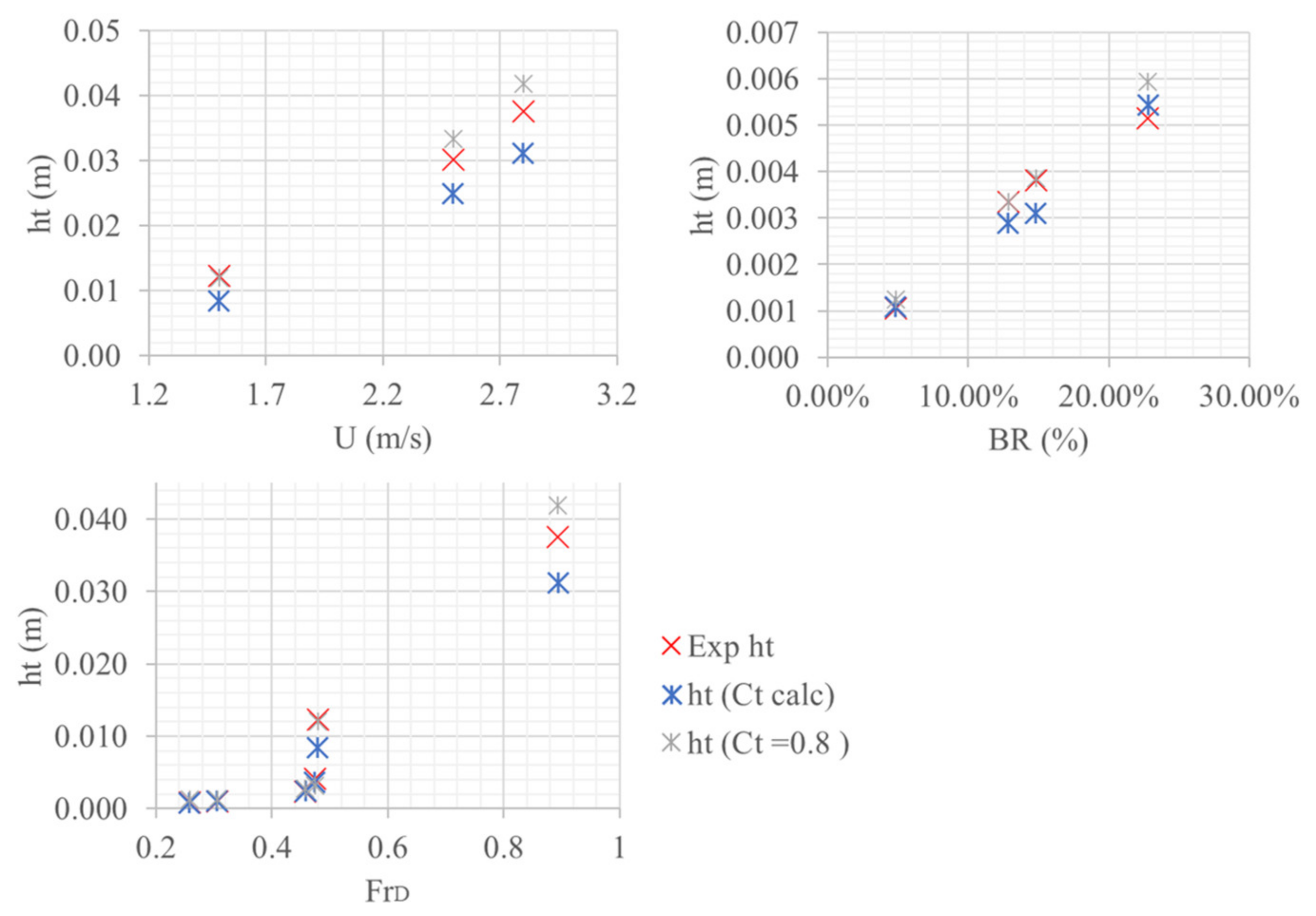
• At turbine optimal operational points, a maximum deviation of 13% from the predicted backwater was obtained when using the correct C_t value. This deviation increased to 19% for the C_t = 0.8 approximation.
• When utilizing the C_t assumption of 0.8, a conservative result was obtained, with the backwater estimation generally overestimating the measured blockage.
• Calculating C_t based on the turbine thrust (measured thrust) lowered the h_t approximation. However, for test cases operating close to the optimal performance and highest C_t value, the backwater was underestimated by up to 20%.
• Test cases at low operational velocities (low Froude numbers) resulted in larger errors in approximating h_t; however, it is important to note that these are unfavourable installation conditions and far from typical installations. The turbines may have low performance at these low operational velocities and, therefore, pose an unrealistic scenario. Here, the C_t calculation resulted in a more realistic value, due to the reduced performance.
• The C_t approximation resulted in large overestimations of the h_t at lower TSRs. However, the C_t equation (Equation (22)) performed well in these scenarios, as the turbine thrust was significantly lower, and the C_t assumption did not hold.
• The C_t approximation gave significantly better results for the three-bladed turbines. The two-bladed (T1) case predicted better results with the C_t calculation, which was also higher than the 0.8 approximation, indicating that the turbine operates closer to the Betz limit and ideal induction factor (a), which could be further tested and calibrated. The C_t calculation performed better in this case, predicting C_t = 0.89. Therefore, utilizing this assumption may be favourable for avoiding errors—especially when turbines with higher operational tip speed ratios are used.

Based on the small dataset obtained from the three turbine models, a C_t value for each turbine can be determined empirically, which could be improved with a larger dataset.

The recommended model also performed significantly better than models found in the literature, as well as needing less input data and background knowledge on specific turbine performance. This indicates the usefulness of this approximation.

5. Conclusions

Quantifying the backwater resulting from the effective blockage caused by the operating turbine remains a challenge for the deployment of HK turbines in inland infrastructure, such as canal systems. This paper shows a simple analytical model to estimate the effective blockage and backwater effect from HK devices. The development of the model followed a similar approach to what has been previously used for bridge pier modelling and quantifying blockages from such structures.

Three variations of typical examples of commercially available HK devices were modelled using a recommended CFD approach, and conditions were varied to allow testing over a range of operational conditions. The water surface profile measurements from the Reference Model 1 (RM1) scaled model experiments allowed validation of the water surface deformation obtained when using a VOF approach coupled with an RS-LPS2 Reynolds stress closure model and BEM-VD blade modelling approach. This highlights the usefulness of CFD models in HK energy development.

The developed backwater model allows a conservative approach with various levels of certainty attainable, depending on the input parameters installed. Although the recommended procedure is an extremely simplified approximation, the results obtained were significantly closer to available dataset of backwater effects than the methods found in the literature. The ease of use also makes this method useful for engineers and developers when detailed numerical models are not feasible.

This model also allows cumulative estimation of backwater, with simple inclusion of blockage structures or multiple turbines using available approximations such as the Yarnell equation. Additionally, due to the nature of flow in canals (flat slopes), subcritical conditions govern, and backwater effects extend a large distance upstream. This allows simple cumulative inclusion of blockages without complex computational modelling, making this approach simple and relatively accurate (or at least favourably conservative).

This approach allows room for further development and determination of calibrated thrust coefficients for typical turbines or typical operational conditions (similar to what was previously done for pier shapes, etc.). Additionally, a similar approach may be investigated for cross-flow turbines where experimental results are available.

Although this paper focussed on backwater determination, other free-surface effects—such as the water level drop over the turbine, or possible hydraulic jumps downstream—are important considerations for array designs. Recommendations for clearance coefficients and turbine spacing (due to wake recovery) should be carefully considered prior to deployment.

References

1. Niebuhr, C.M.; van Dijk, M.; Bhagwan, J.N. Development of a design and implementation process for the integration of hy-drokinetic devices into existing infrastructure in South Africa. Water SA 2019, 45, 434–446. [Google Scholar] [CrossRef] [Green Version]
2. Riglin, J.D. Design, Manufacture and Prototyping of a Hydrokinetic Turbine Unit for River Application. Master’s Thesis, Lehigh University, Bethlehem, PA, USA, 2016. [Google Scholar]
3. Runge, S. Performance and Technology Readiness of a Freestream Turbine in a Canal Environment. Ph.D. Thesis, Cardiff University, Cardiff, UK, 2018. [Google Scholar]
4. Kartezhnikova, M.; Ravens, T.M. Hydraulic impacts of hydrokinetic devices. Renew. Energy 2014, 66, 425–432. [Google Scholar] [CrossRef] [Green Version]
5. Gunawan, B.; Roberts, J.; Neary, V. Hydrodynamic Effects of Hydrokinetic Turbine Deployment in an Irrigation Canal. In Proceedings of the 3rd Marine Energy Technology Symposium, Washington, DC, USA, 27–29 April 2015; pp. 1–6. [Google Scholar]
6. Bahaj, A.S.; Myers, L.E.; Rawlinson-Smith, R.I.; Thomson, M. The effect of boundary proximity upon the wake structure of horizontal axis marine current turbines. J. Offshore Mech. Arct. Eng. 2011, 134, 021104. [Google Scholar] [CrossRef]
7. Bachant, P.; Wosnik, M. Effects of Reynolds Number on the Energy Conversion and Near-Wake Dynamics of a High Solidity Vertical-Axis Cross-Flow Turbine. Energies 2016, 9, 73. [Google Scholar] [CrossRef] [Green Version]
8. Turnock, S.R.; Phillips, A.B.; Banks, J.; Nicholls-Lee, R. Modelling tidal current turbine wakes using a coupled RANS-BEMT approach as a tool for analysing power capture of arrays of turbines. Ocean Eng. 2011, 38, 1300–1307. [Google Scholar] [CrossRef] [Green Version]
9. Mycek, P.; Gaurier, B.; Germain, G.; Pinon, G.; Rivoalen, E. Experimental study of the turbulence intensity effects on marine current turbines behaviour. Part II: Two interacting turbines. Renew. Energy 2014, 68, 876–892. [Google Scholar] [CrossRef] [Green Version]
10. Hill, C.; Neary, V.S.; Guala, M.; Sotiropoulos, F. Performance and Wake Characterization of a Model Hydrokinetic Turbine: The Reference Model 1 (RM1) Dual Rotor Tidal Energy Converter. Energies 2020, 13, 5145. [Google Scholar] [CrossRef]
11. Lalander, E.; Leijon, M. In-stream energy converters in a river—Effects on upstream hydropower station. Renew. Energy 2011, 36, 399–404. [Google Scholar] [CrossRef]
12. Myers, L.; Bahaj, A.S. Wake studies of a 1/30th scale horizontal axis marine current turbine. Ocean Eng. 2007, 34, 758–762. [Google Scholar] [CrossRef]
13. Adamski, S.J. Numerical Modeling of the Effects of a Free Surface on the Operating Characteristics of Marine Hydrokinetic Turbines. Ph.D. Thesis, University of Washington, Washington, DC, USA, 2013. [Google Scholar]
14. Henderson, F.M. Open Channel Flow; The Mcmillan Company: New York, NY, USA, 1966. [Google Scholar]
15. Birjandi, A.H.; Bibeau, E.L.; Chatoorgoon, V.; Kumar, A. Power measurement of hydrokinetic turbines with free-surface and blockage effect. Ocean Eng. 2013, 69, 9–17. [Google Scholar] [CrossRef]
16. Niebuhr, C.; van Dijk, M.; Neary, V.; Bhagwan, J. A review of hydrokinetic turbines and enhancement techniques for canal installations: Technology, applicability and potential. Renew. Sustain. Energy Rev. 2019, 113, 109240. [Google Scholar] [CrossRef]
17. Whelan, J.I.; Graham, J.M.R.; Peiró, J. A free-surface and blockage correction for tidal turbines. J. Fluid Mech. 2009, 624, 281–291. [Google Scholar] [CrossRef]
18. Polagye, B.L. Hydrodynamic Effects of Kinetic Power Extraction by In-Stream Tidal Turbines; University of Washington: Washington, DC, USA, 2009. [Google Scholar]
19. Bryden, I.; Grinsted, T.; Melville, G. Assessing the potential of a simple tidal channel to deliver useful energy. Appl. Ocean Res. 2004, 26, 198–204. [Google Scholar] [CrossRef]
20. Chanson, H. Hydraulics of Open Channel Flow, 2nd ed.; Elsevier Science & Technology: Amsterdam, The Netherlands, 2004. [Google Scholar]
21. Mańko, R. Ranges of Backwater Curves in Lower Odra. Civ. Environ. Eng. Rep. 2018, 28, 25–35. [Google Scholar] [CrossRef] [Green Version]
22. Garrett, C.; Cummins, P. The efficiency of a turbine in a tidal channel. J. Fluid Mech. 2007, 588, 243–251. [Google Scholar] [CrossRef] [Green Version]
23. Garrett, C.; Cummins, P. The power potential of tidal currents in channels. Proc. R. Soc. A Math. Phys. Eng. Sci. 2005, 461, 2563–2572. [Google Scholar] [CrossRef]
24. Ross, H.; Polagye, B. An experimental assessment of analytical blockage corrections for turbines. Renew. Energy 2020, 152, 1328–1341. [Google Scholar] [CrossRef] [Green Version]
25. López, Y.; Contreras, L.; Laín, S. CFD Simulation of a Horizontal Axis Hydrokinetic Turbine. Renew. Energy Power Qual. J. 2017, 1, 512–517. [Google Scholar] [CrossRef]
26. Laín, S.; Contreras, L.T.; López, O. A review on computational fluid dynamics modeling and simulation of horizontal axis hydrokinetic turbines. J. Braz. Soc. Mech. Sci. Eng. 2019, 41, 375. [Google Scholar] [CrossRef]
27. Adcock, T.A.; Draper, S.; Nishino, T. Tidal power generation—A review of hydrodynamic modelling. J. Power Energy 2015, 229, 755–771. [Google Scholar] [CrossRef]
28. Nishino, T.; Willden, R.H. Effects of 3-D channel blockage and turbulent wake mixing on the limit of power extraction by tidal turbines. Int. J. Heat Fluid Flow 2012, 37, 123–135. [Google Scholar] [CrossRef]
29. Nishino, T.; Willden, R.H.J. Two-scale dynamics of flow past a partial cross-stream array of tidal turbines. J. Fluid Mech. 2013, 730, 220–244. [Google Scholar] [CrossRef] [Green Version]
30. Gotelli, C.; Musa, M.; Guala, M.; Escauriaza, C. Experimental and Numerical Investigation of Wake Interactions of Marine Hydrokinetic Turbines. Energies 2019, 12, 3188. [Google Scholar] [CrossRef] [Green Version]
31. Sanderse, B.; van der Pijl, S.P.; Koren, B. Review of computational fluid dynamics for wind turbine wake aerodynamics. Wind Energy 2011, 14, 799–819. [Google Scholar] [CrossRef] [Green Version]
32. Whale, J.; Anderson, C.; Bareiss, R.; Wagner, S. An experimental and numerical study of the vortex structure in the wake of a wind turbine. J. Wind Eng. Ind. Aerodyn. 2000, 84, 1–21. [Google Scholar] [CrossRef]
33. Pyakurel, P.; Tian, W.; VanZwieten, J.H.; Dhanak, M. Characterization of the mean flow field in the far wake region behind ocean current turbines. J. Ocean Eng. Mar. Energy 2017, 3, 113–123. [Google Scholar] [CrossRef]
34. Masters, I.; Chapman, J.C.; Willis, M.R.; Orme, J.A.C. A robust blade element momentum theory model for tidal stream tur-bines including tip and hub loss corrections. J. Mar. Eng. Technol. 2014, 10, 25–35. [Google Scholar] [CrossRef] [Green Version]
35. Guo, Q.; Zhou, L.; Wang, Z. Comparison of BEM-CFD and full rotor geometry simulations for the performance and flow field of a marine current turbine. Renew. Energy 2015, 75, 640–648. [Google Scholar] [CrossRef]
36. Malki, R.; Masters, I.; Williams, A.J.; Croft, N. The variation in wake structure of a tidal stream turbine with flow velocity. In Proceedings of the MARINE 2011, IV International Conference on Computational Methods in Marine Engineering, Lisbon, Portugal, 28–30 September 2011. [Google Scholar] [CrossRef]
37. Edmunds, M.; Williams, A.; Masters, I.; Croft, N. An enhanced disk averaged CFD model for the simulation of horizontal axis tidal turbines. Renew. Energy 2017, 101, 67–81. [Google Scholar] [CrossRef] [Green Version]
38. Masters, I.; Williams, A.; Croft, T.N.; Togneri, M.; Edmunds, M.; Zangiabadi, E.; Fairley, I.; Karunarathna, H. A Comparison of Numerical Modelling Techniques for Tidal Stream Turbine Analysis. Energies 2015, 8, 7833–7853. [Google Scholar] [CrossRef] [Green Version]
39. Masters, I.; Malki, R.; Williams, A.J.; Croft, T.N. The influence of flow acceleration on tidal stream turbine wake dynamics: A numerical study using a coupled BEM–CFD model. Appl. Math. Model. 2013, 37, 7905–7918. [Google Scholar] [CrossRef]
40. Niebuhr, C.; Schmidt, S.; van Dijk, M.; Smith, L.; Neary, V. A review of commercial numerical modelling approaches for axial hydrokinetic turbine wake analysis in channel flow. Renew. Sustain. Energy Rev. 2022, 158, 112151. [Google Scholar] [CrossRef]
41. Mycek, P.; Gaurier, B.; Germain, G.; Pinon, G.; Rivoalen, E. Experimental study of the turbulence intensity effects on marine current turbines behaviour. Part I: One single turbine. Renew. Energy 2014, 66, 729–746. [Google Scholar] [CrossRef] [Green Version]
42. Hill, C.; Neary, V.S.; Gunawan, B.; Guala, M.; Sotiropoulos, F.U.S. Department of Energy Reference Model Program RM1: Experimental Results; University of Minnesota: Minneapolis, MN, USA, 2014. [Google Scholar]
43. Nasef, M.H.; El-Askary, W.A.; AbdEL-hamid, A.A.; Gad, H.E. Evaluation of Savonius rotor performance: Static and dynamic studies. J. Wind Eng. Ind. Aerodyn. 2013, 123, 1–11. [Google Scholar] [CrossRef]
44. Franke, J.; Hirsch, C.; Jensen, A.G.; Krus, H.W.; Schatzmann, P.S.; Miles, S.D.; Wisse, J.A.; Wright, N.G. Recommendations on the use of CFD in wind engineering. In Proceedings of the CWE2006 Fourth International Symposium Computational Wind Engineering, Yokohama, Japan, 16–19 July 2006. [Google Scholar]
45. Malki, R.; Williams, A.; Croft, T.; Togneri, M.; Masters, I. A coupled blade element momentum—Computational fluid dynamics model for evaluating tidal stream turbine performance. Appl. Math. Model. 2013, 37, 3006–3020. [Google Scholar] [CrossRef] [Green Version]
46. Bekker, A.; Van Dijk, M.; Niebuhr, C.M. A review of low head hydropower at wastewater treatment works and development of an evaluation framework for South Africa. Renew. Sustain. Energy Rev. 2022, 159, 112216. [Google Scholar] [CrossRef]
47. Shen, W.Z.; Mikkelsen, R.; Sørensen, J.N.; Bak, C. Tip loss corrections for wind turbine computations. Wind Energy 2005, 8, 457–475. [Google Scholar] [CrossRef]
48. Speziale, C.G.; Sarkar, S.; Gatski, T.B. Modelling the pressure-strain correlation of turbulence: An invariant dynamical systems approach. J. Fluid. Mech. 1991, 227, 245–272. [Google Scholar] [CrossRef]
49. Sarkar, S.; Lakshmanan, B. Application of a Reynolds stress turbulence model to the compressible shear layer. AIAA J. 1991, 29, 743–749. [Google Scholar] [CrossRef] [Green Version]
50. Roache, P.J. Perspectvie: A method for Uniform Reporting of Grid Refinement Studies. J. Fluids Eng. Trans. ASME 1994, 116, 405–413. [Google Scholar] [CrossRef]
51. Silva, P.A.S.F.; De Oliveira, T.F.; Brasil Junior, A.C.P.; Vaz, J.R.P.P.; Oliveira, T.F.D.E.; Junior, A.C.P.B.; Vaz, J.R.P.P. Numerical Study of Wake Characteristics in a Horizontal-Axis Hydrokinetic Turbine. Ann. Braziian Acad. Sci. 2016, 88, 2441–2456. [Google Scholar] [CrossRef] [Green Version]
52. Gibson, M.M.; Launder, B.E. Ground effects on pressure fluctuations in the atmospheric boundary layer. J. Fluid Mech. 1978, 86, 491–511. [Google Scholar] [CrossRef]
53. Neary, V.S.; Gunawan, B.; Hill, C.; Chamorro, L.P. Near and far field flow disturbances induced by model hydrokinetic tur-bine: ADV and ADP comparison. Renew. Energy 2013, 60, 1–6. [Google Scholar] [CrossRef]
54. Yarnell, D. Bridge Piers as Channel Obstructions; United States Department of Agriculture: Washington, DC, USA, 1934. [Google Scholar]
55. Azinfar, H.; Kells, J.A. Backwater Prediction due to the Blockage Caused by a Single, Submerged Spur Dike in an Open Channel. J. Hydraul. Eng. 2008, 134, 1153–1157. [Google Scholar] [CrossRef]
56. Martin-Vide, J.; Prio, J. Backwater of arch bridges under free and submerged conditions. J. Hydraul. Res. 2005, 43, 515–521. [Google Scholar] [CrossRef]
57. Follett, E.; Schalko, I.; Nepf, H. Momentum and Energy Predict the Backwater Rise Generated by a Large Wood Jam. Geophys. Res. Lett. 2020, 47, e2020GL089346. [Google Scholar] [CrossRef]
58. Kocaman, S. Prediction of Backwater Profiles due to Bridges in a Compound Channel Using CFD. Adv. Mech. Eng. 2014, 6, 905217. [Google Scholar] [CrossRef]
59. Azinfar, H.; Kells, J.A. Drag force and associated backwater effect due to an open channel spur dike field. J. Hydraul. Res. 2011, 49, 248–256. [Google Scholar] [CrossRef]
60. Raju, K.R.; Rana, O.; Asawa, G.; Pillai, A. Rational assessment of blockage effect in channel flow past smooth circular cylinders. J. Hydraul. Res. 1983, 21, 289–302. [Google Scholar] [CrossRef]
61. Morandi, B.; Di Felice, F.; Costanzo, M.; Romano, G.; Dhomé, D.; Allo, J. Experimental investigation of the near wake of a horizontal axis tidal current turbine. Int. J. Mar. Energy 2016, 14, 229–247. [Google Scholar] [CrossRef]
62. Jeffcoate, P.; Whittaker, T.; Boake, C.; Elsaesser, B. Field tests of multiple 1/10 scale tidal turbines in steady flows. Renew. Energy 2016, 87, 240–252. [Google Scholar] [CrossRef]
63. Stallard, T.; Collings, R.; Feng, T.; Whelan, J. Interactions between tidal turbine wakes: Experimental study of a group of three-bladed rotors. Philos. Trans. R. Soc. A Math. Phys. Eng. Sci. 2013, 371, 20120159. [Google Scholar] [CrossRef] [PubMed]
64. Lam, W.-H.; Chen, L. Equations used to predict the velocity distribution within a wake from a horizontal-axis tidal-current turbine. Ocean Eng. 2014, 79, 35–42. [Google Scholar] [CrossRef]
65. Sandia National Laboritories: Refernce Model Porject (RMP). Available online: https://energy.sandia.gov/programs/renewable-energy/water-power/projects/reference-model-project-rmp/ (accessed on 21 January 2022).
Figure 1. Water surface profile through a scaled turbine operating at 2 different velocities, compared to the no-energy-extraction stage [12].
Processes 10 01310 g001
Figure 2. Wake expansion effect with free surface [12].
Processes 10 01310 g002
Figure 3. Backwater effect due to turbine blockages [1].
Processes 10 01310 g003
Figure 4. Influence of artificial energy extraction on speed and depth of flow [19].
Processes 10 01310 g004
Figure 5. Water surface deformation from HK devices in inland flow infrastructure.
Processes 10 01310 g005
Figure 6. Computational domain with grid refinements: (A) near wake, (B) blades, and (C) free surface.
Processes 10 01310 g006
Figure 7. Comparison of experimental and computational water surface profiles for the RM1 tests: (a) experiment and CFD water surface graphics; (b) lateral WSE comparison; (c) longitudinal centreline WSE comparison.
Processes 10 01310 g007
Figure 8. Workflow of backwater model development.
Processes 10 01310 g008
Figure 9. Momentum approach schematic (adapted form [55]).
Processes 10 01310 g009
Figure 10. Energy approach.
Processes 10 01310 g010
Figure 11. (a,b) Velocity and (c,d) surface water measurements graphics for the RM1 full model vs. the RM1 rotor and nacelle only.
Processes 10 01310 g011
Figure 12. Pressure measurements over the horizontal and vertical planes (at the turbine hub height centerline).
Processes 10 01310 g012
Figure 13. Pressure measurements over the disk and planes upstream and downstream of the RM1 turbine and retaining structure.
Processes 10 01310 g013
Figure 14. Effects of U, BR, and FrD on the determined ht values.
Processes 10 01310 g014