Article

Renewable Fuels from Integrated Power- and Biomass-to-X Processes: A Superstructure Optimization Study

1
Artec Sustainability Research Center, University of Bremen, Enrique-Schmidt-Straße 7, 28359 Bremen, Germany
2
Advanced Energy Systems Institute, University of Bremen, Enrique-Schmidt Straße 7, 28359 Bremen, Germany
3
SPT-PSE, University of Twente, 7522NB Enschede, The Netherlands
*
Author to whom correspondence should be addressed.
Processes 2022, 10(7), 1298; https://doi.org/10.3390/pr10071298
Submission received: 30 May 2022 / Revised: 22 June 2022 / Accepted: 27 June 2022 / Published: 30 June 2022
(This article belongs to the Special Issue Biomass Conversion Process and Biorefinery)

Abstract

:
This work presents a superstructure optimization study for the production of renewable fuels with a focus on jet fuel. Power-to-X via the methanol (MTJ) and Fischer–Tropsch (FT) route is combined with Biomass-to-X (BtX) via an algae-based biorefinery to an integrated Power- and Biomass-to-X (PBtX) process. Possible integration by algae remnant utilization for H2/CO2 production, wastewater recycling and heat integration is included. Modeling is performed using the novel Open sUperstrucTure moDeling and OptimizatiOn fRamework (OUTDOOR). Novel methods to account for advanced mass balances and uncertain input data are included. Economic optimization proposes a PBtX process. This process combines algae processing with MTJ and depicts a highly mass- and energy integrated plant. It produces fuels at 211 EUR/MWhLHV (ca. 2530 EUR/t), a cost reduction of 21% to 11.5% compared to stand-alone electricity- or bio-based production at algae costs of 25 EUR/tAlgae-sludge and electricity costs of 72 EUR/MWh. Investigation of uncertain data indicates that a combination of BtX and MTJ is economically superior to FT for a wide parameter range. Only for high algae costs of >40 EUR/tAlgae-sludge stand-alone electricity-based MTJ is economically superior and for high MTJ costs above 2000–2400 EUR/tJet FT is the optimal option.

1. Introduction

Due to the urgent threat of climate change induced by anthropogenic greenhouse gas (GHG) emissions, various countries have set out targets for an extensive reduction in CO2 and other GHG. In some sectors such as electricity generation, the defossilization is progressing fast in countries such as Germany, achieving shares of renewable energy production of about 50% in 2020. However, other sectors such as the (petro)chemical industry as well as the mobility sector are much harder to defossilize.
There are already a plethora of different renewable processes to produce petroleum and petrochemical products such as jet fuel as diesel but also platform chemicals, such as light olefins, aromatics or methanol. Bio-based processes (Biomass-to-X = BtX) such as biorefineries utilize energy crops but also waste streams, lignocellulose materials and even micro- and macro algae to produce fuels and biochemicals [1,2]. Electricity-based processes, so-called Power-to-X (PtX) processes, apply water electrolysis in combination with carbon capture to produce mixtures of hydrogen (H2) and carbon dioxide (CO2), that serve as reacting agent in methanol or Fischer–Tropsch synthesis to produce hydrocarbons [3]. However, each process alternative has its own characteristics in terms of cost, utility demands, efficiency or consumption of raw materials such as fresh water.
In order to find an optimal (sustainable) process design, the different concepts have to be compared to each other under specific boundary conditions. What is more, not only should stand-alone processes be reviewed, but also partly or totally integrated Power- and Biomass-to-X processes (PBtX) have to be considered, leading to a vast number of potential process designs.
One way to investigate optimal process designs where many different process layouts are available is the application of superstructure optimization. Superstructure optimization is a methodology for process synthesis which utilizes mathematical models and optimization algorithms to identify optimal process flowsheets for given objective functions [
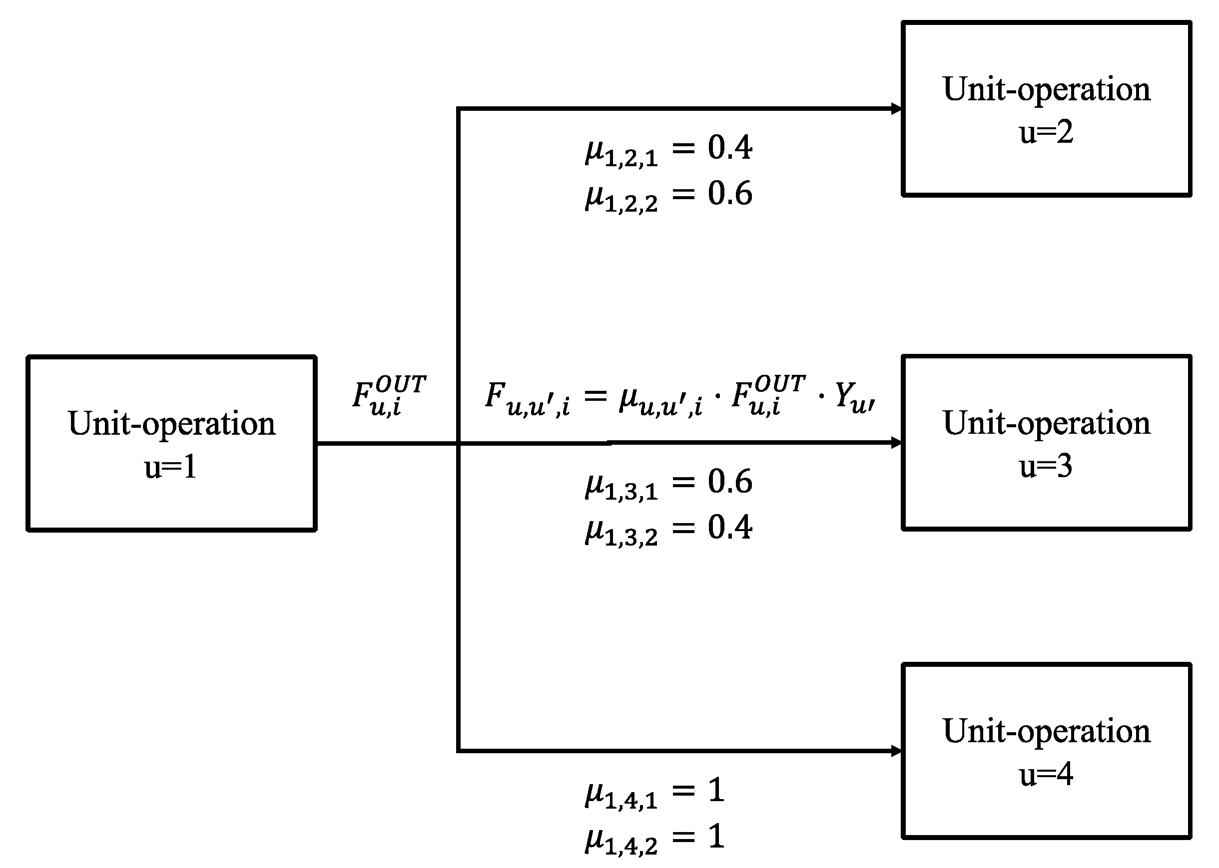
4]. A superstructure represents a large number of possible flowsheets, where unit-operations are described as generic blocks by mass, energy and cost balances [4,5]. Using mathematical modeling, the unit-operations and possible flowsheets are translated into a mathematical program which can be solved using state-of-the art optimization solvers [1,6].
Relevant work regarding superstructure optimization in the area of biorefinery process design was carried out by Gong and You, Bertran et al., Galanopoulos et al., Niziolek et al. and Onel et al. Gong et al. utilized superstructure optimization to identify cost- and emission optimal algae biorefineries producing biodiesel, green diesel and other value-added products [7]. They concluded that manufacturing algal bioproducts reduces GHG by 63% compared to the petrochemical counterparts. Combining biodiesel production with value-added products also reduces the costs of the biodiesel to the level of cost-competitiveness to other biodiesel products. Galanopoulos et al. combined a biorefinery based on wheat-straw for the production of bioethanol and levulinic acid with an algae-based biorefinery for biodiesel and glycerol production. The integration of wastewater and CO2 from wheat-straw refinery as a raw material in algae cultivation and the recycling of algae remnant as a raw material for bioethanol production results in a cost reduction of about 40% for open pond cultivation [8]. Niziolek et al. investigated the bio-based production of aromatics via methanol amongst others. Their superstructure includes biomass gasification, methanol synthesis, methanol-to-aromatics and several recycling schemes for light gases such as combustion for energy production or conversion in autothermal reforming. Different biomass feedstocks are studied, namely corn stover, switchgrass and hardwood. They calculate payback times of roughly 9 years for the most profitable process configuration. Onel et al. set up a superstructure using forest residues and natural gas to produce liquid transportation fuels and olefins by utilizing the Fischer–Tropsch route [9]. They also incorporated heat, power and water integration in their model. They concluded that the optimal process configuration depends on the desired fuels and olefins and that such a combined production could lead to economic viability [9].
In the field of PtX superstructure optimization work has been performed by Sanchez et al., Uebbing et al. and Kenkel et al. [10,11,12]. Sánchez et al. investigated a superstructure of ammonia-based electricity production. In their problem, decisions on gas clean-up after electricity production in a combined gas and steam turbine as well as final N2/Air separation are made. The MINLP uses detailed sub-models for, e.g., ammonia decomposition and aims to minimize operation costs of power production. Results show that power production costs can vary between 0.05 and 0.81 EUR/kWh depending on plant capacity and ammonia price [10]. Uebbing et al. investigated a CO2 methanation superstructure combining biogas processing and water electrolysis to provide synthetic natural gas for the gas grid. They combine detailed unit models with indirect heat integration and optimized for maximal exergetic efficiency and minimal capital costs. Results show that using solid oxide electrolysis for H2 supply has a higher exergetic efficiency than using alkaline electrolysis [11]. However, this comes at the price of substantial higher capital costs. Kenkel et al. investigated bi-criteria power-to-methanol process designs with different CO2 sources and different electrolyzer types in combination with direct hydrogenation of CO2 to methanol [12]. In their work, green methanol is produced cost-optimally by a combination of low-pressure alkaline electrolysis, CO2 from flue gases captured by amine scrubbing and utilization of purge gases for steam production. Using this process layout methanol is produced at ca. 900 EUR/t, with H2 supply contributing over 70% of the total costs [12].
In addition to superstructure-based studies, several conventional techno-economic studies on the production of liquid fuels have been performed by Schemme et al., Liebner et al., Albrecht et al. and König et al. among others [3,13,14,15]. Schemme et al. investigated costs of several H2 process routes for fuels such as gasoline, diesel and DME. They conclude that DME is the cheapest option with ca. 1.85 EUR/lDiesel equivalent [14]. Liebner et al. compare their MtSynFuels process with the Fischer–Tropsch route for the production of fuels and calculate production of roughly 180 $/t using natural gas as raw material [14]. Albrecht et al. propose a standardized method for techno-economic evaluation of alternative fuels and demonstrate it on a combined Power-and Biomass-to-X process using the Fischer–Tropsch route including PEM electrolysis and biomass pyrolysis among other technology steps. They estimate fuel production costs in the range of 1.2–2.8 EUR/l [3]. König modeled a Fischer–Tropsch process for the production of jet fuel and calculated costs at 3.38 EUR/kg [15].
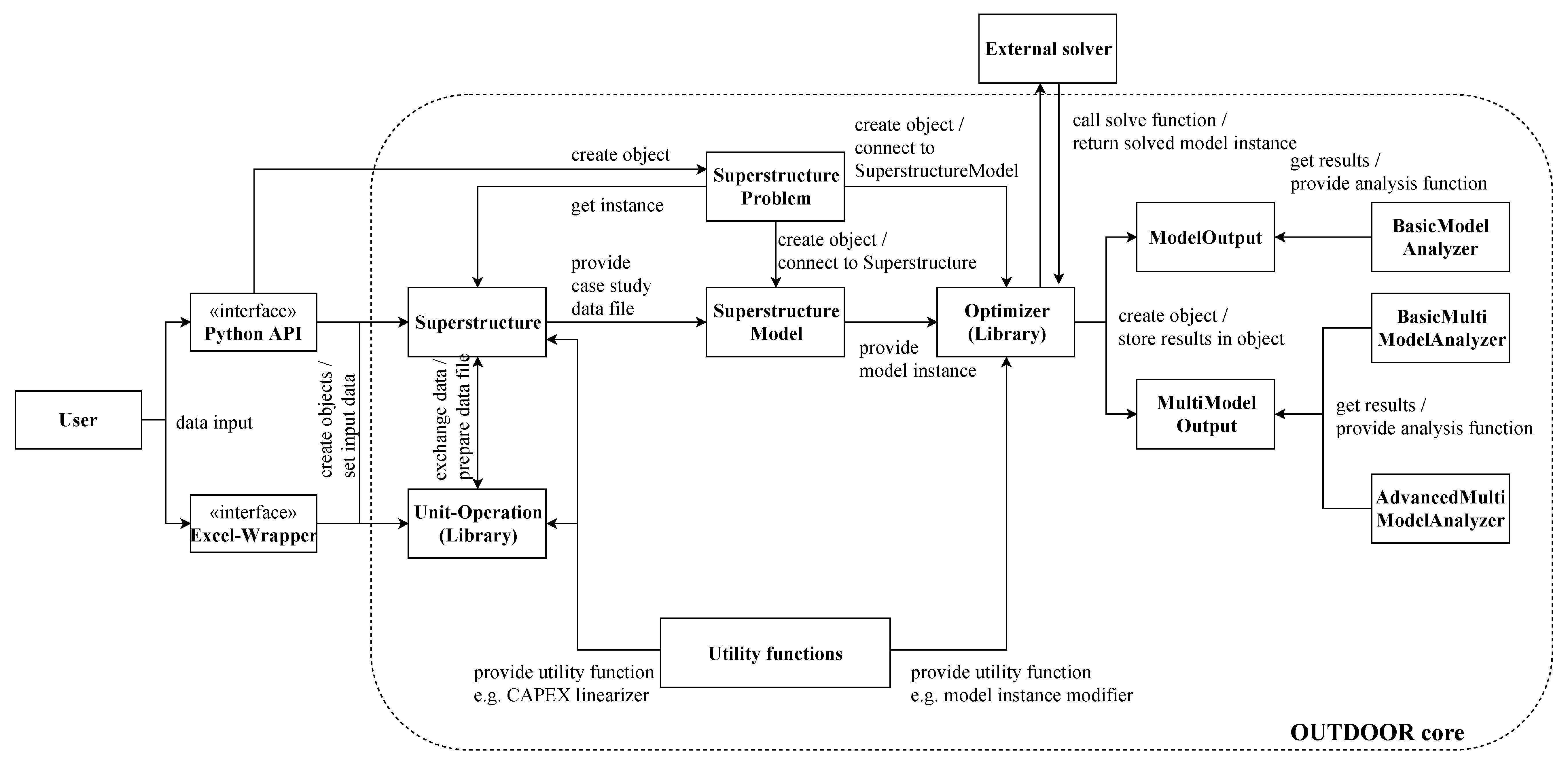
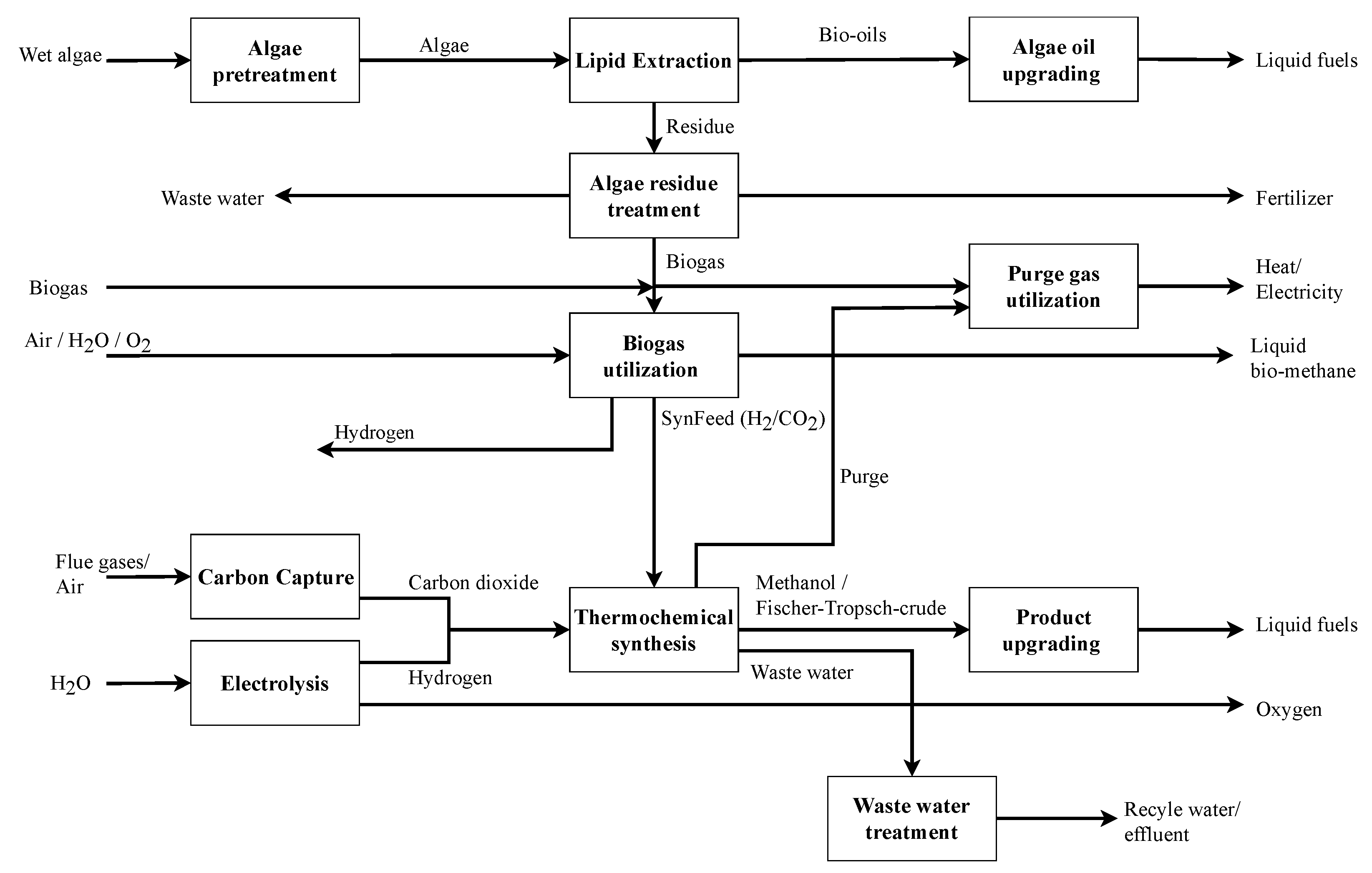
While PtX as well as BtX and even PBtX processes a have been investigated, no superstructure optimization has been performed to find optimal integrated PBtX process designs for the production of jet fuel as one major mid- to long term required liquid fuel in the transport sector. To close this knowledge gap, we present a superstructure optimization study, which aims to find cost optimal process designs from an integrated PBtX jet fuel refinery. This renewable refinery combines HEFA (hydroprocessed esters and fatty acids) production from microalgae as well as remnant biogas processing together with water electrolysis, carbon capture and thermochemical conversion of H2/CO2 to jet fuel via the methanol (methanol-to-jet = MTJ) or Fischer–Tropsch (FT) route. Such a comprehensive superstructure has not been investigated in literature yet, and the deep integration of PtX and BtX processes, including novel technologies with uncertain data requires an advanced modeling approach as well as methodologies to handle the emerging uncertainties. In the course of this study, the Open sUperstrucTure moDeling and OptimizatiOn fRamework (OUTDOOR), a python-based superstructure modeling and optimization tool is enhanced to facilitate such complex investigations.
This paper is structured as follows: First, the superstructure of the integrated refinery is described in detail (Section 2), then the problem statement and solution approach are given (Section 3). Section 4 presents the results of the process synthesis and gives a discussion on the cost efficiency of novel processes as well as integrated concepts. Finally, a conclusion is presented and further investigation is proposed.

2. Process Description

The general layout of the superstructure is depicted in Figure 1. It includes 11 main processing steps. The bio-based pathway includes a biorefinery using algae biomass as raw material to produce HEFA as main product, with minor shares of gasoline and diesel as by-products. The PtX pathway includes different water electrolysis and carbon capture technologies to produce H2 and CO2 with subsequent methanol or Fischer–Tropsch synthesis, including their respective upgrading to jet fuel and further by-products. A combined PBtX process is realized by integrating algae residue conversion to SynFeed (H2/CO2 mixture) as input for thermochemical synthesis as well as combined wastewater management, purge gas utilization and heat integration. The detailed processing steps and considered technology options of the renewable refinery are described in detail in the following section.

2.1. Power-to-X Process

Electricity-based fuel production uses carbon capture processes for pure CO2 production as well as water electrolysis for H2 production with oxygen (O2) by-product. H2 and CO2 are consumed in thermochemical synthesis by either methanol synthesis or Fischer–Tropsch synthesis. Produced intermediates are afterwards upgraded depending on the primary synthesis to liquid fuels.

2.1.1. Carbon Capture

The carbon capture section provides CO2 as a raw material for thermochemical synthesis. Three different technologies, namely low temperature direct air capture (LT-DAC), oxyfuel fired cement factory with subsequent cooling and water separation (OXY) as well as oil refinery flue gas scrubbing using monoethanolamine (MEA-CC) are included in the superstructure [16,17,18]. While LT-DAC and MEA-CC produce low-pressure CO2 at 1 bar, OXY internally prepares the carbon dioxide at 70 bar. As shown in Figure 2 the low-pressure CO2 streams are mixed with potential flows from a CO2-distributor (CO2-DIST) and compressed to high pressure for thermochemical synthesis.

2.1.2. Water Electrolysis

Water electrolysis provides the H2 feedstock for thermochemical synthesis as well as hydrotreating processes. Included technologies are high- and low-pressure alkaline electrolysis (HP-AEL/AEL) at 30 and 1 bar, high-pressure proton exchange membrane electrolysis (HP-PEMEL) at 30 bar and solid oxide electrolysis (SOEL) at ambient pressure (see Figure 3). While PEMEL and AEL operate at low temperatures of around 70 °C and are powered solely by electricity, SOEL operates at elevated temperatures up to 1000 °C where part of the energy input is introduced as steam. Therefore, electricity demand varies from 4.4 kWh/Nm3 to 4.9 kWh/Nm3 and capital costs from 700 EUR/kWel to 3000 EUR/kWel [19,20,21]. It is assumed that all electrolyzer technologies achieve total conversion, meaning that 1 kg of water is converted to 0.112 kg of H2 and 0.888 kg of O2 (see Equation (1)).
H 2 O   0.112   H 2 + 0.888   O 2  
Three H2 compressors with different compression ratios are included in this superstructure. A first one compresses ambient-pressure H2 to methanol operating pressure of 70 bar (H2-LH-COMP) using multiple stages. A second compressor provides a single-stage compression from 30 bar to 70 bar (H2-MH-COMP) in order to connect HP-AEL and HP-PEMEL to methanol synthesis. A third compressor depicts a single-stage compression of ambient-pressure H2 to medium pressure of 30 bar (H2-LM-COMP). High-pressure hydrogen at 70 bar is solely used in methanol synthesis. However, medium- (30 bar) and low- (1 bar) pressure H2 has several applications in the process structure. Therefore, both streams are connected to their distinct distributing units MP- H2-DIST and LP- H2-DIST. Low-pressure H2 can be distributed to the H2-LM-COMP and H2-LH-COMP as well as being used in energy integration, where it is combusted with other purge gases to produce either steam (HEAT GEN) or electricity (EL GEN). In addition to compression to 70 bar, medium-pressure hydrogen is the electricity-based feed for Fischer–Tropsch synthesis. However, it is also used in the deoxygenation of bio-oil (BIO-U), hydrotreating of methanol-to-jet intermediates (MTJ) and Fischer–Tropsch crude hydrocracking (FT-C). Additionally, it can also be used in HEAT GEN and EL GEN as well as sold as by-product (H2-Pool). Emerging O2 can either be sold as by-product or used in processes such as the oxyfuel cement factory carbon capture and autothermal as well as tri-reforming of bio-methane and biogas (further explained in BtX process sections).

2.1.3. Thermochemical Synthesis and Upgrading

The thermochemical product synthesis is either chosen as methanol synthesis or as Fischer–Tropsch synthesis route (see Figure 4).
Methanol synthesis is implemented as direct hydrogenation of CO2 at 70 bar and 250 °C. It is modeled using a three-step surrogate process. This process includes the main methanol reactor (MEOH SYN), a flash evaporation (MeOH FLASH) to separate purge gas of inert and unreacted components as well as a final distillation column (MeOH DC) which purifies the raw methanol by separating wastewater. Arising purge gas is further treated in the purge gas treatment section, while wastewater is processed in a wastewater treatment plant (WWT). The surrogate model is based on a detailed model provided by Wassermann et al. with yield factors of the methanol reaction, as given in Table 1. [18].
The pure methanol is upgraded using the general concept of methanol-to-jet based on consecutive methanol-to-olefins, olefins oligomerization and hydrofinishing. The product distribution (given in Table 2) as well as hydrogen demand in hydrotreating are based on the MtSynfuels process described by Liebner et al. [14]. The hydrofinishing step requires ca. 0.004 t H2/tMeOH. Here, again wastewater is separated and treated in WWT for recycling or disposal.
The FT route is modeled after the work of König and depicts a conversion with jet fuel as the main product [15]. The detailed model was again consolidated to a limited number of unit-operations. First, the raw materials are mixed (FT-M), afterwards CO2 and H2 are converted to synthesis gas by reverse water-gas-shift reaction at temperatures of 900 °C (RWGS). The required heat is provided internally by fuel gas combustion and small amounts of additional steam. The synthesis gas is afterwards converted to Fischer–Tropsch crude, waxes, wastewater and fuel gas in a FT-reactor at 225 °C and approximately 25 bar (FT-R). The fuel gas produced is used as a heating agent of the RWGS in a burner (FT-B). The wastewater generated in the FT synthesis is sent to the wastewater treatment plant. Crude and waxes are afterwards upgraded. Crude is sent directly to product splitting via distillation. Waxes are first hydrocracked with a H2 demand of 0.006 t H 2 / t Waxes . Afterwards, the produced intermediate is also sent to the distillation column. Here, liquid fuels are again separated and a small share of additional fuel gas is generated, which is sent to the FT-B. The yield factors of the main Fischer–Tropsch reaction as well as FT-upgrading and MTJ process are given in Table 2.
The capital costs for the MTJ are between 300–700 EUR/tJet (if scaled down to small scale) [14]. Capital costs for small scale FT synthesis are reported to be between 270 and 800 EUR/tJet [13,14,15]. Additionally, Liebner states that MTJ can deliver a 15% cost reduction in comparison to FT synthesis in small scale. Considering König’s rather conservative data for FT synthesis of approximately 780 EUR/tJet, costs for MTJ are assumed to be roughly 85% of this value, leading to base case capital costs of 660 EUR/tJet. Considering the 20-year plant lifetime and 5% interest to calculate the capital recovery factor and assuming 10% of yearly operational costs based on the fixed capital investment, total processing costs of ca. 1500 EUR/tJet are taken as base value (Equation (2)).
C M T J = 660 EUR t + 660   EUR / t C R F · 10 % = 1485   1500   EUR / t Jet

2.2. Biomass-to-X Process

The BtX process pathway is two-fold in this superstructure. The first path utilizes biogas from a biogas plant with a composition of 65 vol. -% CH4 and 35 vol. -% CO2 for the production of SynFeed in thermochemical synthesis. The second pathway depicts an algae-based biorefinery to produce hydroprocessed esters and fatty acids (HEFA) from the algae lipids, while recycling algae residue for either anaerobic digestion or combustion. While the biogas plant is limited to 3.5 t/h (ca. 3000 Nm3/h), depicting a large size bio-methane plant, the capacity of the biorefinery is unlimited.

2.2.1. Algae Raw Material

The biorefinery pathway uses microalgae biomass to produce liquid fuels from the algae-oil as well as biogas, recycle water and solid fertilizer from the remaining carbohydrates, protein and water shares. Industrial algae cultivation is a process that is still under development and subject to a broad scientific discussion. Different cultivation reactor concepts from open ponds, over photo-bioreactors and thin-layered cascade reactors exist. Additionally, different strains of algae differ greatly in terms of productivity, lipid content or even applied culture broth. The literature reports productivity values from 5 to a maximum of 60 g/m2/d, while lipid content can rise up to 50 or even 70 wt.-% [22,23]. On top of that, microalgae can be clustered into freshwater and saline strains, where the former can also be used to treat municipal wastewater, while the latter is not dependent on fresh water reserves [24,25]. During cultivation algae are strongly diluted with about 0.15 g/L to 4 g/L in open ponds and photo-bioreactors [26]. To effectively use the biomass, it has to be harvested and dewatered. A typical primal harvesting technology is the sedimentation basin which can increase the biomass concentration up to 1%. Afterwards, technologies such as dissolved air flotation can be used to further increase biomass concentration to 10% [27]. Further dewatering can be achieved using mechanical filter presses or centrifugation which increase dry biomass concentrations to 20–30% [28]. For complete dewatering, different drying technologies can be used [28]. However, they are energy-intensive. Thus, algae-sludge is often further processed with a concentration of 20–30%.
Due to this broad spectrum of raw material and processing alternatives, thw literature reports algae production costs between 145 and 1315 EUR/tDry-mass [22].
Because of the variety of technology options as well as scarcely available detailed techno-economic models in the literature, the wet algae biomass is simply modeled as a raw material which is produced on-site in this superstructure. It is assumed that the algae-sludge is harvested and dewatered using conventional processes leading to a dry matter concentration of 10 wt.-%. Algae costs of 265 EUR/tDry-mass based on results from Davis et al. serve as base case costs [22]. These costs can be affiliated with a large-scale production with cultivation productivity of 25 g/m2/d [22]. Assuming 10 wt.-% dry biomass this leads to 26.5 EUR/tAlgae-sludge which is rounded to 25 EUR/tAlgae-sludge. Davis et al. use the Scenedesmus acutus strain of algae which has a molar chemical composition of CH1.82O0.49N0.03S0.001P0.002 [22]. Next to about 30% lipids the biomass consists of 2.4% ash, ca. 53% carbohydrates 13% proteins and 1.6% further cell mass [22]. However, they also mention the well-known Chlorella vulgaris strain, which has a more or less similar composition with slightly lower lipids concentration and higher carbohydrates content. It is often discussed as major strain in biodiesel production [29]. In order to keep the generic character of the algae production process the lipid content as well as the costs of algae-sludge are varied in the later optimization study, thus showing more general effects and not specifically for one chosen algae strain. Table 3 gives an overview of the key parameters of the algae raw material.

2.2.2. Biomass Pretreatment and Lipid Extraction

Typical micro algae for fuels production exhibit lipid contents of 25 wt.-%. However, only a certain share of those oils is directly available. Some is mixed with other components and stored in cell walls, which reduces the amount of extractable oil. To break intercellular walls and increase the available oil content, a pretreatment step can be included. Additionally, this step increases the availability of the ligno-cellulosic residue for anaerobic digestion. Various technologies from physical to thermal and chemical concepts are available. Some examples are high-pressure homogenization, microwaving or milling and grinding. For a broad overview we refer to Kamperidou et al. [30].
In this superstructure a sonication process (SONIC) is implemented (see Figure 5). It is assumed that 50% of the lipids are available without pretreatment. Using sonication, the available share can be increased to 96% [7].
To separately use the lipids and algae residue, an extraction step is necessary. Oil extraction is commonly performed by chemical extraction using non-polar solvents. Two process alternatives are implemented: The commonly known hexane extraction (HEX-EXT) and the more advanced supercritical CO2 extraction (SUP-CO2-EXT) (see Figure 5). While the hexane extraction only extracts 35% of the available oils, supercritical CO2 extraction has an efficiency of 100% [7]. However, the energy consumption of this alternative is also substantially higher.

2.2.3. Bio-Oil Upgrading

The extracted bio-oil is upgraded based on the UOP refining process (BIO-U). This process includes hydrotreating, hydrocracking and isomerization as well as product distillation. The data of the techno-economic model are extracted from Klein-Marcuschamer et al. [2]. His process design considers a three-stage hydrodeoxygenation reactor at 350 °C to produce saturated alkanes and propane. Afterwards, the alkanes are further treated by hydrocracking and hydro-isomerization. Unreacted hydrogen is recovered and cleaned using amine scrubbing, before internal recycling. The product distribution of the process is depicted in Table 4. The total hydrogen demand is 0.158 t H 2 / t Bio oil . During amine scrubbing, high purity CO2 is produced. Because capital cost data was only based on rough estimates, the complete process design is modeled as one surrogate unit-operation in the superstructure model. This unit-operation includes the complete data such as yield factors, energy demand and capital costs.

2.2.4. Biogas Utilization and SynFeed Upgrading

After lipid extraction, remaining algae biomass and water can be further exploited (see Figure 6). The wet residue is converted into biogas by anaerobic digestion (AAD). Afterwards the gaseous stream and the liquid stream are separated. The liquid stream contains water with diluted salts and remaining solid compounds. The solid compounds are separated from the liquid using centrifugation (CENTR) and can be sold as fertilizer [7]. The water can be purified and used as a raw material for electrolysis or directly used as a cultivation medium in algae cultivation. The second option suggests a co-location of algae biomass production and renewable refinery, as it is assumed in this work. The gaseous product of anaerobic digestion is raw biogas with a composition of 65 vol. -% CH4 and 35 vol. -% CO2 [7]. This biogas can be further utilized. Therefore, a biogas distributor (BG-DIST) is used to distribute among the biogas utilization or the purge gas treatment section.

2.2.5. Biogas Utilization and SynFeed Upgrading

Biogas from anaerobic digestion of algae residue as well as biogas raw material from the biogas plant can be processed in similar ways (see Figure 7). The simplest way to combust biogas to produce energy (further described in purge gas treatment section).
Additionally, three different reforming technologies are included in the superstructure: Steam methane (SMR) and autothermal (ATR) reforming of bio-methane as well as direct biogas tri-reforming produce a CO2/H2 mixture which can be used as feed material for the thermochemical synthesis (therefore called SynFeed). To utilize SMR and ATR upstream biogas purification by pressure swing adsorption (BG-PSA) and vacuum pump (VP) separate CO2 [7]. The pure CO2 stream can be mixed with low-pressure CO2 from carbon capture to provide raw material for thermochemical synthesis, or it just can be vented to the environment. SMR, ATR and TRIR are similar in that they include a series of reforming steps, namely pre-reforming at 500 °C, main reforming to syngas as well as two-stage water-gas-shift reaction at 350 °C and 210 °C to convert CO and H2O to H2 and CO2 [31]. In the end, the raw SynFeed is available at approximately 23 bar and cooled down to 40 °C for compression to 70 bar [31]. Differences in the process design arise in the main synthesis reaction. The SMR unit uses an externally fired isothermal reactor at 890 °C, where heat supply is provided by combustion of a share of the inlet bio-methane [31]. Hot flue gas is used in heat recovery and steam generation to produce excess electricity. ATR and TRIR both utilize partial oxidation using pure oxygen instead of air at temperatures around 1000 °C [31]. Due to internal heat supply, no excess heat is produced. The raw SynFeed has to be upgraded to meet the H2/CO2 ratio of the different thermochemical synthesis process options. Therefore, excess hydrogen from SMR is separated by pressure swing adsorption (H2-PSA) and excess CO2 from ATR and TRIR is separated using physical absorption with Selexol as sorbent [31]. H2- and CO2 recovery factors of the given technologies are 89% and 90%, respectively. Independent from the decision on reforming technology and upgrading, the different SynFeed streams are distributed by a set of distributors to Fischer–Tropsch synthesis or compression for methanol synthesis. Fischer–Tropsch synthesis operates at the pressure outlet of the reforming technologies. To use the SynFeed in methanol synthesis a compressor (SYNFEED COMP) is included. The techno-economic models of the reforming technologies, upgrading sections and compressions are taken from a previous study on biogas reforming [31].
In addition to reforming, bio-methane can be liquified at –152 °C by a reversed Rankine process (BM-LIQ). The resulting liquefied bio-methane depicts a liquid fuel. However, it is only considered as a by-product in this work due to the major difference in handling and transportation compared to the other fuels. Additionally, the liquifying process does not produce aviation fuel (shares), which is the main goal of the process layout. Data for the liquification from of bio-methane is taken from Capra et al. [32].

2.2.6. Purge Gas and Wastewater Treatment

Depending on the final process layout, different combustible gases arise, which have to be burned in order to keep emissions of unreacted hydrocarbons to a minimum as well as to increase the overall energy efficiency of the process. These gases are the purge stream from methanol synthesis, raw biogas from either algae remnant treatment or raw material (biogas plant) as well as H2-by-products. Gases can either be burned to produce steam for internal heat supply (HEAT GEN) or electricity by application of a combined cycle power plant (EL GEN) (see Figure 8) [7].
Arising wastewater from distillation columns, compression intercooling or from wet algae biomass can be recycled and used again in processes such as electrolyzers or as steam input for biogas reforming processes. Another option is to release remaining water into the environment as effluent. Anyway, in both cases wastewater has to be purified first in order to reduce impurities and potential remaining hydrocarbons. Wastewater treatment is not modeled in detail but is considered to cost 2.5 EUR/t [3].

2.2.7. Raw Materials, Distributors, Products

Raw materials include biogas from the biogas plant with an input limit of 3.5 t/h, as well as different flue gases, pure O2, wet algae-sludge, process water, air, monoethanolamine and hexane. Except for the biogas raw material, none of the raw materials is limited in terms of availability. External O2 is assumed to be produced using cryogenic air separation.
The main products of the process system are the fuel products. The main products are jet fuel, gasoline, diesel and LPG. The process alternatives derive the exact distribution of fuels. However, in the end, they are summarized under one final product “fuels” with their respective lower heating value. Due to this approach, costs as well as emissions, can be easily allocated to the different main products depending on their energy content. Next to the main fuel pool, by-products include medium-pressure hydrogen, oxygen, solid fertilizer, liquified bio-methane and recycle water for algae cultivation.
A set of 10 distributor units is implemented in the superstructure, which distribute streams according to Table 5.
The flowsheet synthesis is investigated based on generic assumptions. However, relevant data such as electricity or natural gas costs and emission factors are modeled after the German energy system. Table 6 depicts main input parameters. Full load hours were derived from a H2 supply optimization case study by Wassermann et al. [33]. Electricity greenhouse gas (GHG) emissions and fresh water demand (FWD) were calculated based on data from the ecoinvent database [33,34]. They reflect direct electricity purchase from offshore wind farms at the German North Sea with the FLH derived from Wassermann et al. Electricity costs for offshore wind energy are taken from a study published by the Fraunhofer ISE [35]. Steam costs were derived using Aspen Plus simulation and its integrated economic analyzer. The approach assumes natural gas combustion with a cascade of four heat exchangers to produce superheated, high-, medium- as well as low-pressure steam. Natural gas at costs were assumed to be 2.785 ct/kWh [12]. Costs of unit-operations, natural gas and final cooling were allocated to the different steam types based on their energy content. Table 7 presents costs, GHG emissions and FWD of major raw materials and (by-)products.

3. Methodology

3.1. Problem Statement

The following components and parameters of the superstructure model are given:
  • Techno-economic sub-models for different unit-operations including:
    Split factors;
    Concentration requirements;
    Specific utility demands;
    Inlet- and outlet temperatures for heating/cooling demands;
    Capital costs functions;
    Lifetime;
    Cost factors for operation and maintenance, direct- and indirect capital costs;
    For reactor units: Stoichiometric and Yield parameters;
    For combined gas- and steam turbine / steam furnace: Efficiencies.
  • Key parameters (costs, environmental burdens) for external utilities:
    Electricity;
    Steam (super-heated, high-, medium- and low-pressure);
    Cooling water;
    Refrigeration.
  • Total plant full load operating hours (FLH).
  • Interest rate for capital costs calculation.
  • Key parameters for raw materials:
    Composition;
    Purchase costs;
    Environmental input balance;
    Minimum and maximum availability.
  • Key parameters for byproducts:
    Revenues;
    Environmental avoided burdens.
  • Key parameters for high temperature heat pump:
    Coefficient of performance (COP);
    Inlet- and outlet temperature;
    Linear capital costs.
  • Given chemical components and their key parameters:
    CO2 equivalent;
    Lower heating value.
The OUTDOOR mathematical model is used, which implements the following constraints:
  • Mass balances must be met;
  • Splits are fixed based on given parameters for normal unit-operations;
  • Splits are variable for distributor units; the outlet composition is fixed;
  • The main product is a mixture of liquid hydrocarbons with respect to their lower heating value;
  • The yearly production of main product is set to 240,000 MWh which corresponds to 20,000 t/a fuel given a mean lower heating value of 12 MWh/t (43.2 MJ/kg);
  • The model is not time-indexed but works with a fixed annual number of full load hours;
  • A base case is investigated in detail with:
    Algae-sludge costs of 25 EUR/t;
    MTJ processing costs of 1500 EUR/t;
    Electricity price of 72 EUR/MWh;
    Algae lipid content of 25 wt.-%.
  • Four different scenarios are investigated using the developed screening algorithm with:
    Scenario 1: Electricity price of 72 EUR/MWh and lipid content of 25 wt.-%;
    Scenario 2: Electricity price of 36 EUR/MWh and lipid content of 25 wt.-%;
    Scenario 3: Electricity price of 72 EUR/MWh and lipid content of 50 wt.-%;
    Scenario 4: Electricity price of 36 EUR/MWh and lipid content of 50 wt.-%.
  • For every scenario a set of mutable parameters are calculated:
    MTJ processing costs: 680–2800 EUR/t;
    Algae-sludge purchase costs: 5–105 EUR/t.
With the given parameters and constraints, the optimization model minimizes the net production costs of the fuel mixture as calculated in Equation (3). To do so, it also determines:
  • The accurate mass- and energy-balances;
  • The total GHG emissions and fresh water demand;
  • Choice and size of technology;
  • Variable splits for distributor units;
  • Capital and operational costs for the sized unit-operations.
min N P C = C A P E X + O P E X P R O F I T S cap PROD
For the collected data, all costs are implemented as EUR 2020. The complete Excel-based data input sheet can be found in the Supplementary Information S1.

3.2. Solution Approach

To strengthen scientific discussion and the ability to recreate scientific output, the optimization model is created with OUTDOOR (Open sUperstrucTure moDeling and OptimizatiOn fRamework) [42]. OUTDOOR is an open-source python module which combines object-oriented programming and data management with conventional algebraic modeling via the Pyomo modeling language. OUTDOOR models are written as mixed-integer linear programming models (MILP) which allows the usage of different open-source as well as state-of-the art commercial solvers. The base model is extensively presented and discussed by Kenkel et al. [12]. It utilizes different concepts modelling and programming concepts as well as approaches from techno-economic and life cycle analysis calculations [43,44,45,46]. In the course of this work, the modeling framework was extended and the model updated for necessary functions. Below, the general aspects of the framework and the required added functionalities are described. The complete, updated optimization model can also be found in the Supplementary Material S2. The updated version of the python package can be found under https://github.com/PKenkel/OUTDOOR (accessed on 29 May 2022).

3.2.1. OUTDOOR General Modeling Framework

OUTDOOR is a highly object-oriented software which aims for maximum automation in the superstructure modeling and optimization procedure, but also provides a modular toolset for general modeling and optimization purposes. The detailed model architecture with roles and interaction of included classes is given in the Appendix BFigure A2. Below, the superstructure modeling and optimization algorithm which is implemented in OUTDOOR will be shortly explained using Figure 9. First, the user has to input the data of the case study. In order to accelerate and simplify this process, OUTDOOR provides object-oriented classes and data structures. Different unit-operation classes such as stream splitters, reactors or product pools act as blueprints for the unit-operation objects that are necessary. These objects are created and parametrized with data such as specific energy demand, capital cost functions or split factors. Afterwards, the created unit-operation objects are added to an object of the superstructure class. This class depicts the boundary conditions such as plant operating hours per year, electricity prices or yearly desired product load. Object instantiation can be carried out by using a python IDE and the included python API. However, OUTDOOR also comes with a Microsoft Excel-based user interface that provides ready-made Excel sheet templates that can be used to fill in unit-operation and boundary conditions data sets.
When the user included the case study data OUTDOOR’s automated algorithm does the rest independently. The algorithm first creates an empty optimization model, which is an object that inherits from Pyomos AbstractModel class and depicts empty equations describing all substantial correlations of the model: Mass and energy balances, cost functions, emissions and logic constraints. Additionally, the superstructure object is used to generate a data file which depicts the model-readable data version of the case study. The data file and the empty optimization model are used in a third step to create a filled model instance, which then includes all required equations as well as all the required data for the case study. This model instance is afterwards processed by internal optimizer classes which in turn take advantage of external solvers such as Gurobi, Cplex or cbc. After the model is solved, the included data (sets, parameters, calculated variables and objective) are saved into OUTDOOR’s model output class in order to cut down on used memory storage. The model output class saves all data in common python data structures such as lists and dictionaries. Additionally, OUTDOOR provides a set of analyzer classes which are able to perform techno-economic and environmental analysis, create flowsheets, save results as txt-files or create graphs and tables for sensitivity analysis, respectively.
Next to the described capabilities, OUTDOOR provides a set of utility functions which are used by the different classes. These include an automated piecewise-linearizer for non-linear capital cost functions as well as different automated optimization modes such as multi-objective optimization and sensitivity analysis. The selectable predefined objective functions of OUTDOOR’s superstructure model are minimization of net production costs (NPC), net production greenhouse gas emissions (NPE) and net production fresh water demand (NPFWD).

3.2.2. Added Functionalities

Prior to this work, OUTDOOR already provided several functionalities for superstructure modeling and optimization. Nonetheless, some features were missing to investigate process synthesis for highly integrated novel processes. One was a variable distribution of mass flows instead of connections via fixed split factors. This would enable flowsheets that use shares of intermediate products to satisfy demands in other unit-operations while selling the remaining fractions as by-products. The second feature that was missing is an approach to handle uncertain input data and compare competing technology alternatives with respect to this uncertainty. By applying fitting methods, the economics of novel technologies still in the development phase can be compared to each other even if overall processing costs of such options are still uncertain to some level, hence supporting the decision-making in early design phases. Within the scope of this work, both features are developed and integrated in OUTDOOR as presented in the following:

Distributor Units

Normally, unit-operations in OUTDOOR interact with each other by pre-defined specific split factors. These split factors describe separation performance as well as connection between different unit-operations. They are defined for the connection of one process u to another process u′ for every chemical component i. In combination with the requirement of mass balance (see model in Supplementary Information), these split factors build the topology of the superstructure. However, one major disadvantage of pre-defined split parameters is that they bound the topology to (more or less) binary decisions. An example is given in Figure 10, where F u , i O U T is the outlet flow of component i of unit-operation u, μ u , u , i is the pre-defined split factor of component i from unit u to u′ and F u , u , i is the actual flow of component i from unit u to u′ based on the binary decision variable of Y u that depicts the choice of technology. It is clear, from the figure, that the given topology can only result in either choosing to send 40% of i = 1 and 60% of i = 2 to units u = 2 and 60% of i = 1 and 40% of i = 2 to u = 3 or to send the total stream to unit u = 4, otherwise mass balances are disobeyed. When investigating highly integrated processes, this can lead to suboptimal process layouts. Sometimes, it could be beneficial to distribute flows more variable. This can be especially the case if intermediate products are used in other process stages as reacting material. In this case, it could be beneficial to only process the right amount to satisfy the demand, while the rest is, e.g., sold to the market.
In order to model such behavior, we developed the distributor unit, which works in similar way to a multi-target valve. The detailed mathematical formulation can be found in the model, provided in the Supplementary Information. The general concept is depicted for a two-target distributor in Figure 11 and works as follows:
Prior to the optimization target processes, u′ are assigned to the distributor as well as the accuracy of splitting in terms of number of calculated decimal points. During the optimization, the outlet flow F u , i O U T of component i from the distributor u is calculated as the sum of inlet flows coming from connected unit-operations. This outlet flow can be distributed to the targets according to the defined accuracy. While the mass flow split is variable, the composition of each flow is equal. In order to achieve this behavior, the distributor unit is assigned an indexed parameter d u , k D I S T which includes a binary number system (e.g., [0, 0.1, 0.2, 0.4, 0.8, 0.01….]). Multiplication of the indexed parameter with assigned binary variables Y u , u , k D I S T and outlet flow F u , i O U T determines the slack variable F u , u , k , i D I S T . The total split to a target is then derived by the sum of all shares combined with the binary decision variable Y u (see Figure 11). In the final model, bi-linear equations are linearized by Big-M formulations and additional constraints assure mass balance. Using this approach, every distributor unit adds NB binary variables to the model, as shown in Equation (4), where NT is the number of assigned targets and ND the degree of distribution accuracy.
N B = N T   1 + 4 N D

Optimal Design Screening Algorithm

So far, each case study in OUTDOOR is optimized for one of the three predefined objective functions with a fixed parameter set. Additionally, OUTDOOR already includes a functionality to automate sensitivity analysis where one parameter is modified step by step while all other parameters are set constant. However, to compare novel or competing process alternatives with uncertain input data, it can be practical to modify two parameters, e.g., the processing costs of two alternatives at the same time. This so-called two-way sensitivity analysis results in a multi-dimensional solution matrix including outcomes such as minimized costs but also technology choice and flowsheet topology for every parameter pair. In order to create and analyze such a multi-dimensional solution matrix, a screening algorithm, inspecting economic designs is developed and implemented in OUTDOOR. The proposed algorithm combines two-way sensitivity analysis with tailor-made automated graph construction and works as follows:
  • Definition of two parameters (which are, e.g., processing costs of two alternatives);
  • Definition of minimum and maximum value as well as step size for both parameters;
  • Definition of process alternatives which should be screened for;
  • Preparation of N x-values and N y-values based on step one and two;
  • Execution of two-way sensitivity analysis for N x N superstructure models by iteratively:
    • Modification of model instance parameters;
    • Execution of superstructure optimization for given model instance;
    • Extraction of single-optimization results and adding them to multi-dimensional solution matrix;
  • Conversion of technology choice results to numerical scale;
  • Interpretation of multi-dimensional solution matrix for graph creation.
Steps 1–3 have to be performed by the user; step 4–7 are performed automatically by OUTDOOR. To perform the two-way sensitivity analysis, OUTDOOR’s integrated optimizer algorithm first calculates two lists of linearly spaced values for the chosen mutable parameters based on the minimum and maximum value as well as step size. Afterwards, an iteration of parameter modification, superstructure optimization and single-run results file saving is performed until every parameter combination is explored. Parameter modification is implemented as an extension of the already existing sensitivity analysis functionalities. Hence, OUTDOOR’s modular architecture is exploited to keep effort at a minimum level. The total file, containing all results data of every independent optimization is returned as an overall solution file. This multi-model-output object can be connected to one of the aforementioned analyzer classes which includes a method to automatically create a technology choice graph for a maximum of four different processes.
This graph method first extracts the mutable parameter lists and sets up a mesh grid on an x- and y-axis, based on these parameters. Afterwards, the main results, namely calculated net production costs (NPC) and technology choice for every calculated single-optimization are extracted. The NPC are mapped over the mesh grid according to the given parameter set. The technology choice is first translated into numeric values based on the defined technology choices. This is achieved by utilizing a system of binary numbers where single technology choices are references by an ascending binary number and a combination of different choices is assigned the sum of the single numbers. An example is presented in Table 8. In the end, the NPC are plotted as a contour graph on the x,y-meshgrid while the numeric scale of technology choice is plotted as a heatmap with discrete numbers and colors. Figure 12 presents the general mapping of NPC and technology choice from given numbers in a mesh grid to the final graph. This graph provides a simple and intuitive way to analyze technology choice and NPC based on two varying parameters.

4. Results and Discussion

4.1. Model Characteristics and Computational Performance

The superstructure model consists of 685,497 constraints and 24,4823 variables, of which 1600 are binary. The base case optimization was performed on a server using four 2.2 GHz cores with a total RAM of 300 GB available. Utilizing Gurobi 9.1.2 as an optimization solver, the base case takes a total 2033 s resulting in an optimal solution with a 0.01% remaining optimality gap, which is Gurobi’s default threshold. Of those 2033 s, 11% are required by OUTDOOR’s automated superstructure construction and model building, 35% are invested in transferring the python model to the Gurobi solver and 53% are actually required by the solver. It is notable that roughly 16% of the solver time is required in order to reduce the optimality gap from 1% to 0.01%.
The screening algorithm requires numerous sequential optimizations. Therefore, the different scenarios were calculated in parallel on an external server, where each scenario was assigned a maximum number of four 2.2 GHz cores, with a total RAM of 300 GB. During the screening, the single-run solver times vary, depending on the parameter set, and can consume considerably more time (up to >19,000 s) than the base case optimization. In order to reduce calculation time, a remaining optimality gap of 0.1% was allowed for the screening algorithm, leading to total computing times of 42,044 to 87,514 s, depending on the scenario.

4.2. Base Case Results

For the given base case: Electricity costs of 72 EUR/MWh, algae lipid content of 25 wt.-%, algae-sludge costs of 25 EUR/t and MTJ costs of 1500 EUR/t
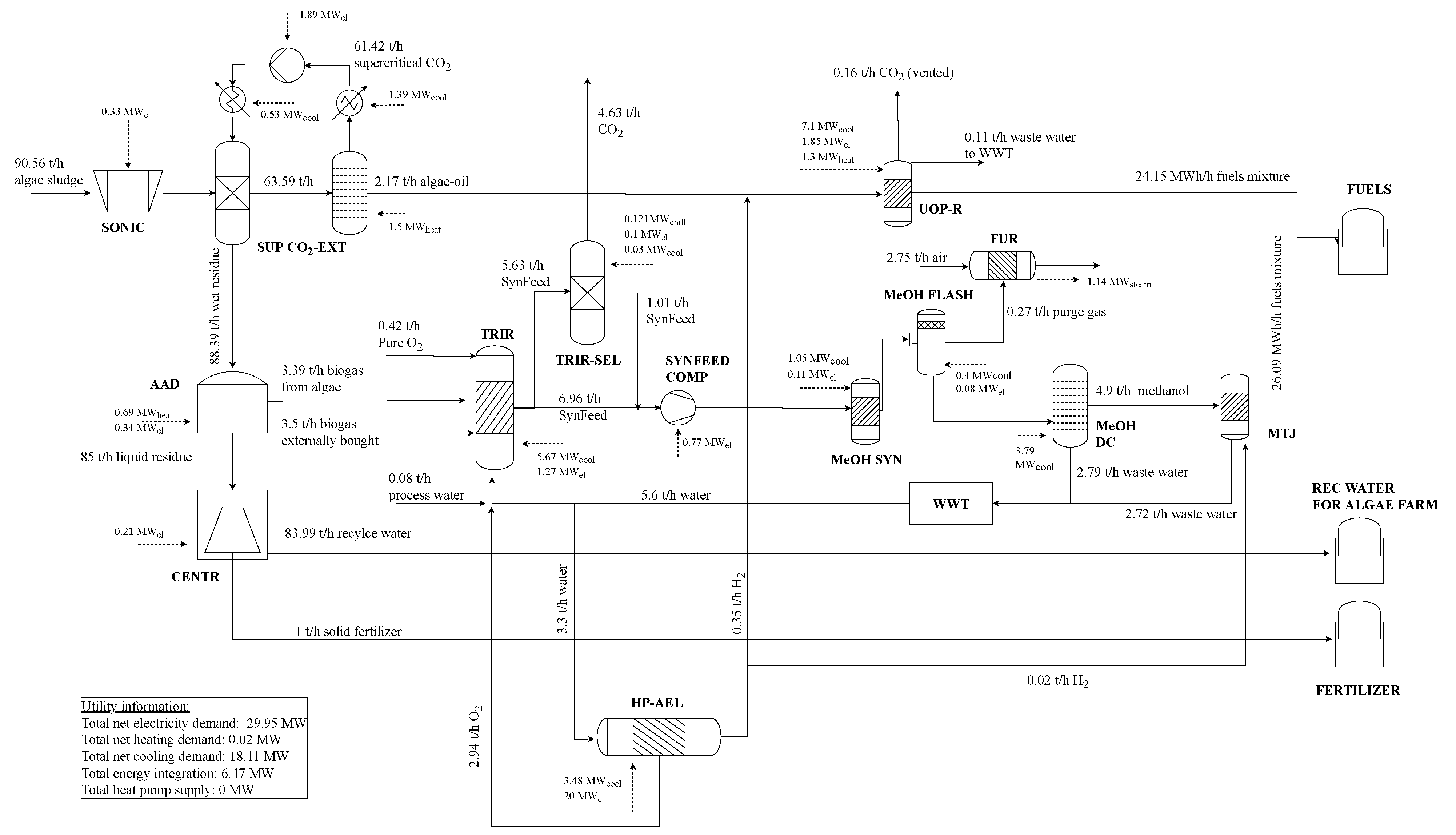
Jet are required for an optimal process design that depicts a highly integrated BtX and PtX process. The detailed flowsheet is depicted in Figure 13. In total 240,000 MWh/a (approximately 20 kt fuels/a) are produced at net production costs of 253 EUR/MWhLHV (approximately 2993 EUR/tFuels). The fuels shares are 47% jet fuel, 23% diesel, 18% gasoline and 12% LPG. Fuels are produced to 52% based on MTJ using algae residue and additional biogas and 48% using hydrotreating of algae bio-oil. Additional CO2 is not used and H
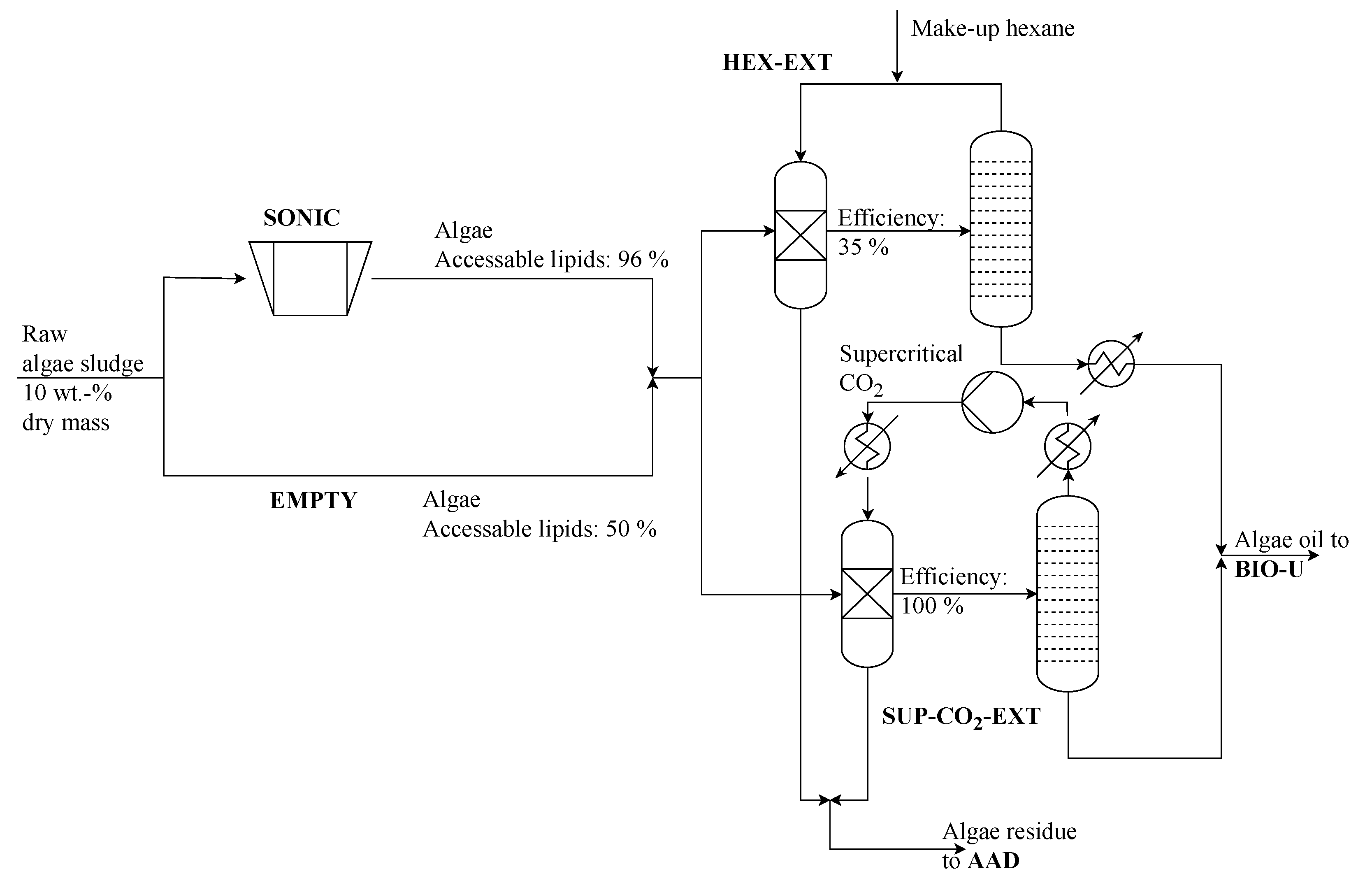
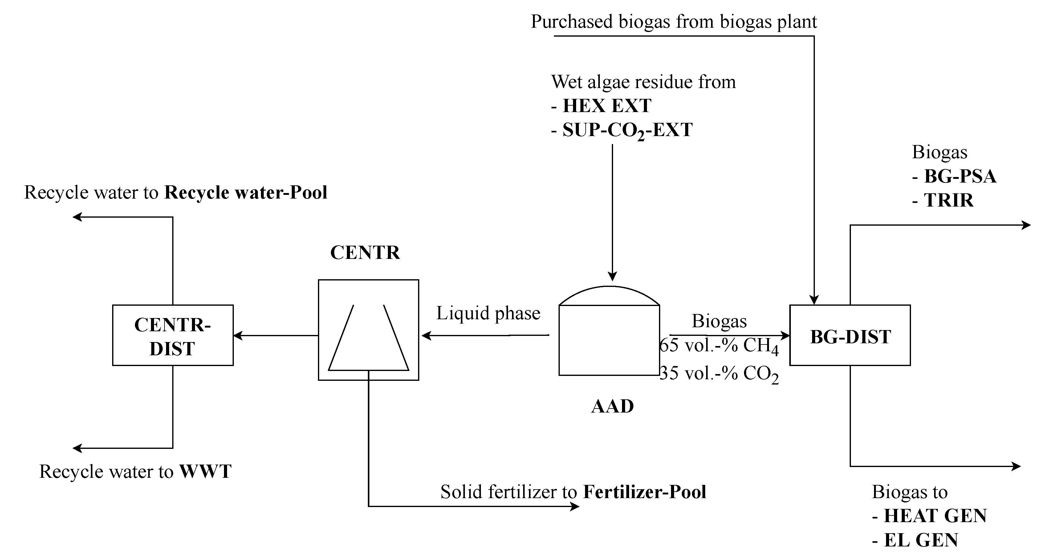
2 from electrolysis is only used in hydrotreating and not as main feed. Algae-sludge is used as raw material and pretreated by sonication. Subsequent lipid extraction is designed as supercritical CO
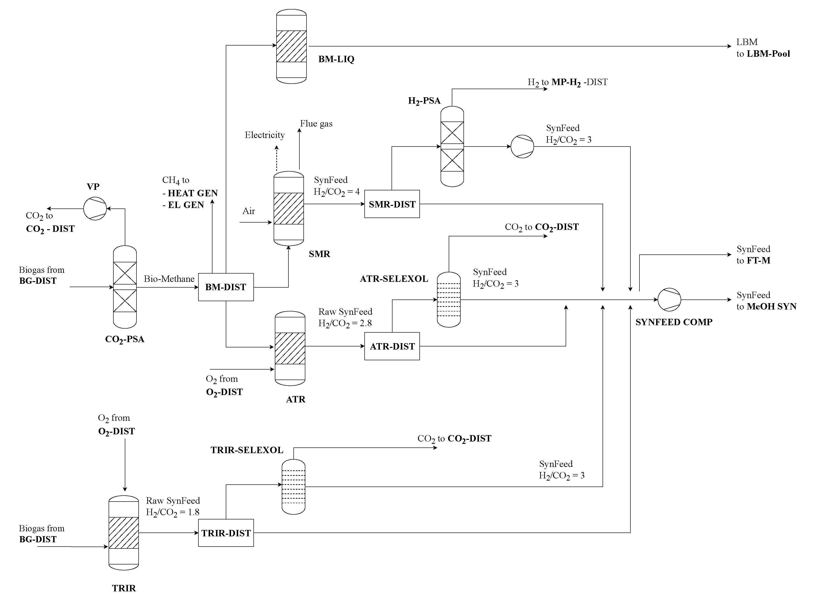
2 extraction. Lipids are afterwards refined to HEFA using hydrodeoxygenation. Algae residue is converted to biogas by anaerobic digestion. Liquid remnants is treated by centrifugation which separates solid fertilizer as a by-product and remaining water for usage in the co-located algae farm. The remaining biogas is mixed with additionally bought biogas from a biogas plant and converted to raw SynFeed by TRIR. Part of the raw SynFeed is upgraded with selexol-based CO2 capture. The captured CO2 is not required anymore and vented. The low-detail model of algae cultivation does not include the acquisition of CO2. However, in the proposed flowsheet, vented CO2 from the TRIR-SEL, BIO-U and HEAT GEN process could provide approximately 30% of the cultivation CO2 demand. The purified SynFeed is mixed with the remaining SynFeed to meet the specification of methanol synthesis. The produced SynFeed is compressed to 70 bar and converted to methanol, and methanol is upgraded to fuels by MTJ. A high-pressure alkaline electrolysis unit produces small amounts of H2 which are utilized in hydrodesoxygenation of bio-oil (BIO-U) and hydrotreating in MTJ. The O
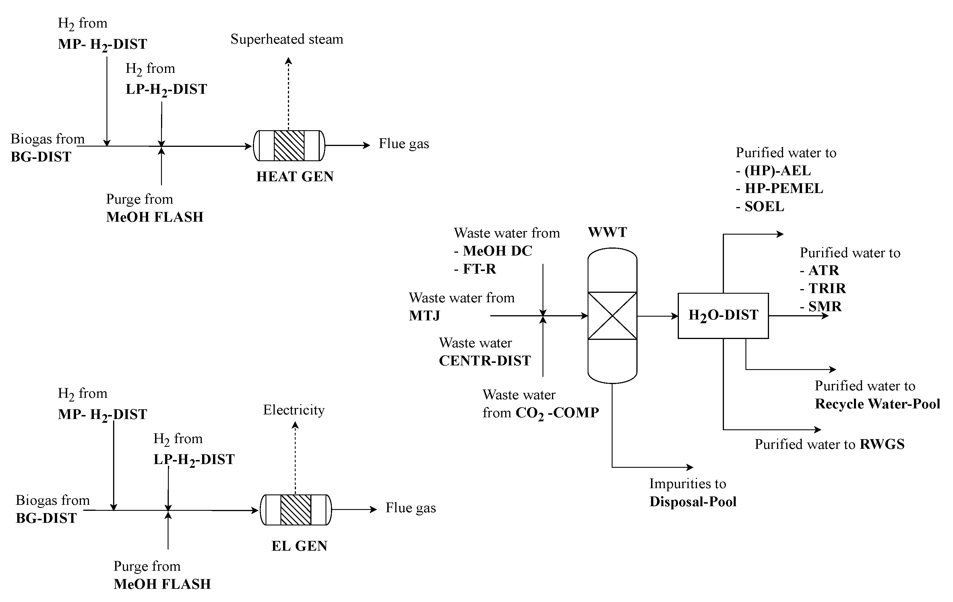
2 by-product of the HP-AEL is used in TRIR to produce the required heat via partial oxidation. Purge gas from the methanol synthesis is combusted to produce superheated steam, which is used to decrease the external steam demand. Wastewater from methanol distillation, MTJ and BIO-U is treated in WWT first, and afterwards used as a raw material in TRIR and HP-AEL.
Heat integration reduces the external heat demand from ca. 6.49 MW to 0.02 MW. Ca 18% of the recovered heat is produced in purge gas treatment and the remaining 82% is gained from waste heat of methanol synthesis and flash as well as hydrodeoxygenation of bio-oils and intercooling of the TRIR process. The model does not include detailed HEX-matching. However, based on the given temperature levels, a first indication of matches can be provided. In such a matching, high-temperature heat from HEAT GEN, MeOH SYN, TRIR and BIO-U would be used for medium temperature demand in BIO-U. Heat from cooling in MeOH FLASH and TRIR would be coupled with the distillation column of the SUP-CO2-EXT. Finally, waste heat from BIO-U or TRIR would be used in the AAD. Additionally, 18.11 MW of cooling utility are required. The total electricity demand is ca. 30 MW, of which 20 MW are required by the HP-AEL.
Table 9 presents the cost breakdown of the NPC. It can be seen that the major cost drivers are capital costs with 43.3% and raw materials with 27.5%; the third and fourth largest share are electricity costs (17%), and operating and maintenance (16.6%).
Figure 14 shows the breakdown of capital costs (left) and electricity demand (right). Largest capital cost shares are generated by MTJ (24.3%), TRIR (15.6%), anaerobic digestion (16.6%) and BIO-U (17.8%).
Electricity is mainly consumed by the high-pressure alkaline electrolysis and the H2 compressor (66.8%) as well as the supercritical CO2 extraction (16.3%). Raw material costs mainly originate from raw algae-sludge purchase (64.7%) and raw biogas (35%).
When comparing the combined PBtX refinery with a purely electricity-based MTJ or FT refinery, a cost reduction ca. 21% and 28% can be achieved, respectively. If compared to a stand-alone biorefinery, where algae residue is converted to a liquid bio-methane by-product, a cost reduction of 11.5% is achieved. A comparison to the literature is not as simple due to the numerous assumptions. Wassermann et al. reported lower MTJ-based jet fuel costs of ca. 2225 EUR/tJet [47]. However, they also used reduced electricity costs of 50 EUR/MWh and lower MTJ process costs of about 400 EUR/tJet based on large scale applications [47]. If both factors are included in the comparison, the total costs of fuel are again in the same range. König calculated FT-based jet fuel prices of 3380 EUR/tFuel [15]. However, he had increased electricity costs of 104 EUR/MWh, but a substantially larger plant with 526 ktJet/a output and high full load hours of 8760 h/a, leading to reduced capital cost shares [15]. In general, all of the results are in the same region depending on the chosen assumptions.
In terms of environmental impacts, the optimal base case comes with negative greenhouse gas emissions of –3.7 t CO 2 / t Fuels , while requiring 960 t H 2 O / t Fuels   of water. When compared to the stand-alone options, greenhouse gas emissions are in the same region for all options. Water demand, on the other hand, is another matter. Algae cultivation requires substantially more water than water electrolysis and carbon capture. Due to avoided burdens for by-products, electricity-based processes even generate negative water demands of ca. –7.5 t H 2 O / t Fuels . Table 10 presents costs and GHG emissions of conventional production of the given yearly product loads considering the actual product distribution and reference GHG emissions and costs from Table 7. Based on these values and the calculated costs and emissions of the renewable refinery, CO2 abatement costs of ca. 561 EUR / t CO 2 arise (see Table 11).

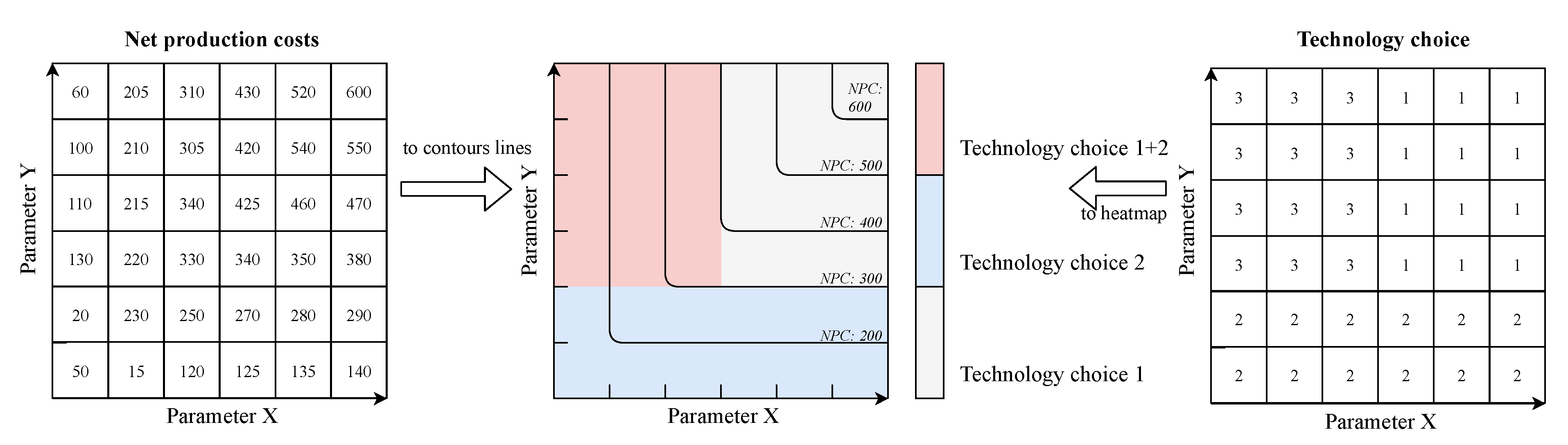
4.3. Optimal Design Screening Algorithm Results
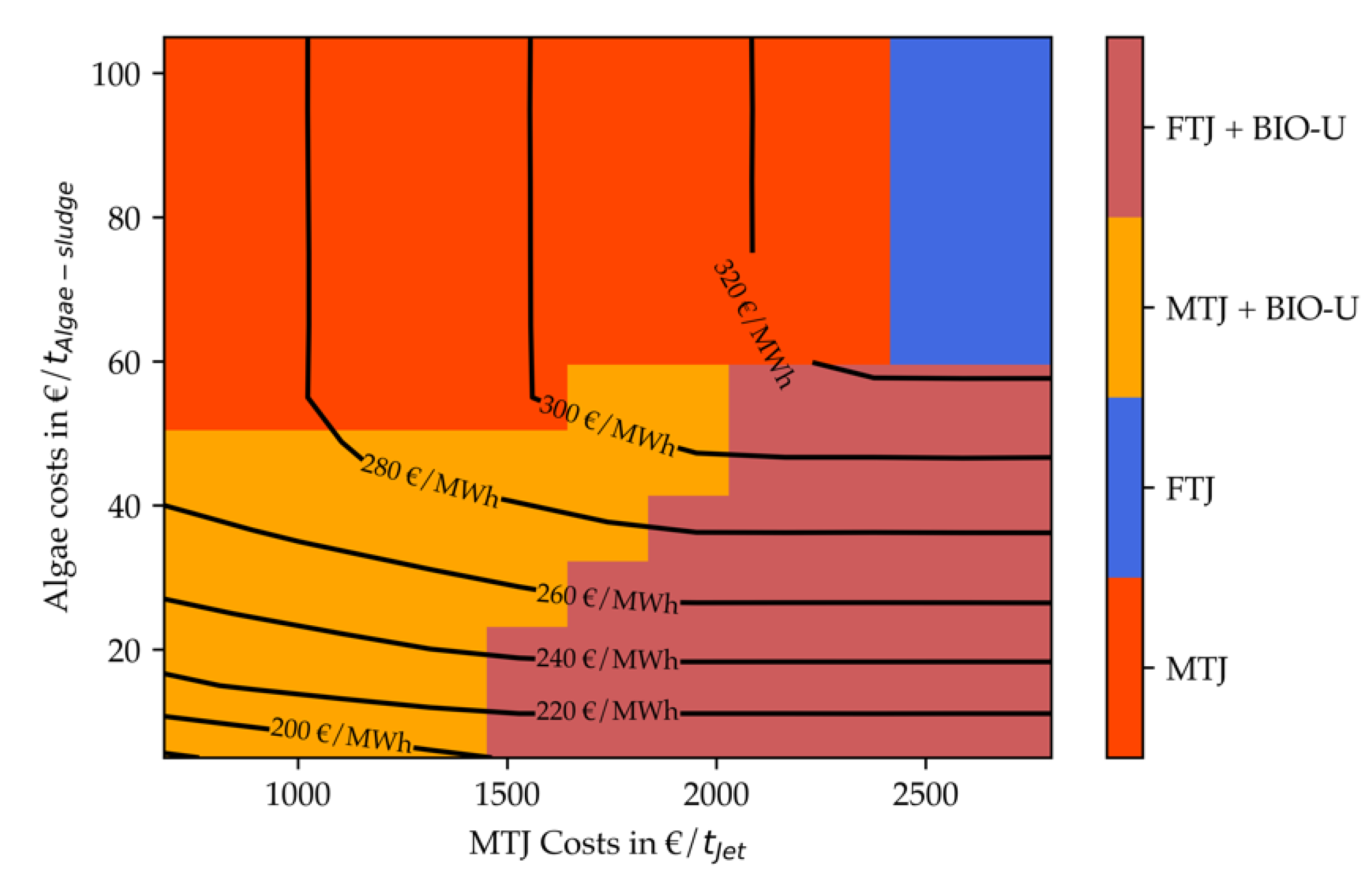
Figure 15 and Figure 16 present the results of the optimal design screening algorithm for the electricity price of 72 EUR/MWh. Figure 15 depicts an algae lipid content of 25 wt.-% and Figure 16 depicts a lipid content of 50 wt.-%.
It can be seen that, for 72 EUR/MWhel and 25% lipids, fuel costs vary between ca. 177 and 331 EUR/MWhLHV (2092–3912 EUR/t) for algae costs between 5 and 105 EUR/tAlgae-sludge and MTJ costs between 680 and 2800 EUR/tJet. Four distinct operating windows appear for different algae costs and total MTJ processing costs. For low algae and MTJ costs, a combination such as presented in the base case is most profitable. For MTJ costs higher then 1500 EUR/tJet, this step is replaced by Fischer–Tropsch synthesis. If algae costs exceed approximately 40 EUR/tAlgae-sludge, a purely electricity-based production is chosen based on methanol synthesis for MTJ costs up to ca. 2400 EUR/tJet. For even higher costs, an FT-based production is most economic.
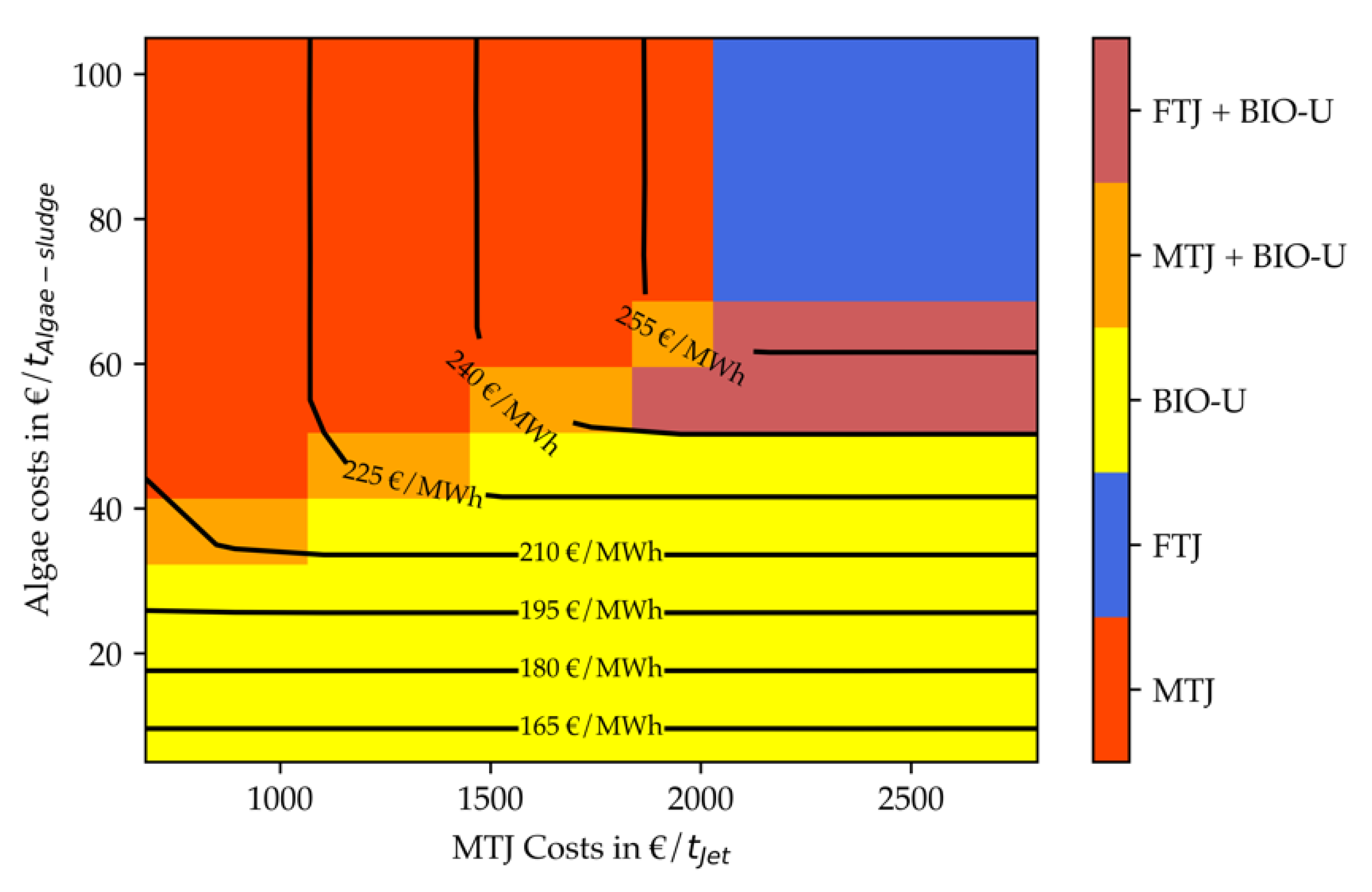
If the lipid content in the raw algae is elevated (Figure 16), the total fuel costs range changes to 2150–3912 EUR/t. The maximum cost value is still associated with a purely electricity-based production; hence it is independent from the lipid content. The minimal price is slightly elevated compared to a lower lipid content. Nonetheless, the costs for combined process concepts are on average about 10% cheaper compared to the case with 25% lipids. This can be explained by the bio-based nature of the combined process: While alkaline electrolysis plays a role in the overall process scheme, the main feedstock for the products is based on algae. If the content of lipids which can be converted directly to fuels rises, this leads to smaller capacities in anaerobic digestion, biogas reforming and MTJ. These processes are the most expensive ones in the total process design, which makes capacity reduction a good cost saver.
Additionally, to the four operating windows recorded previously, now a purely bio-based production is most economic for low algae costs of up to 35 EUR/tAlgae-sludge and MTJ costs higher than 1000–1250 EUR/tJet. Furthermore, the operating window for an integrated design is increased for higher algae costs up to 70–95 EUR/tAlgae-sludge depending on the MTJ costs.
Figure 17 and Figure 18 display the screening results for an electricity price of 36 EUR/MWh. Figure 17 again depicts an algae lipid content of 25%, while Figure 18 depicts a lipid content of 50%. It is evident from Figure 17 the total costs range for decreased electricity price also decreases to ca. 165–263 EUR/MWh (1950–3109 EUR/tFuel). This is equivalent to a 10% to 20% cost reduction compared to the higher electricity price. Especially for purely electricity-based production, the share of electricity costs is high, explaining the increased cost reduction at the high-end of the price range. In general, it can be seen that the operating windows for stand-alone MTJ and FT production processes are increased compared to the cases with higher electricity price. Nonetheless, for low algae costs up to 30–40 EUR/tAlgae-sludge a combination with methanol or Fischer–Tropsch synthesis is still beneficial. As shown in Figure 17, an operating window for a stand-alone biorefinery also emerges for very low algae costs of 5 EUR/tAlgae-sludge and MTJ costs above 1000 EUR/tJet.
Figure 18 shows the results for a lipid content of 50% for a decreased electricity price. It follows the logic of the other graphs. Both stand-alone electricity-based and bio-based production operating windows are increased. For low algae costs, pure algae-based production is most economic. Due to high lipid content, this is the case for algae costs up to 40 EUR/t. The optimal region for integrated process design is very small. Due to the low electricity price, stand-alone MTJ or FT is quickly more economic than a combined process. The total cost range is between 156 and 262 EUR/MWh (1844–3109 EUR/t). The maximum cost value is again similar to scenario 3, due to the independency of the FT process from the algae lipid content. The minimum value is slightly lower, due to more economic usage of algae-oil and lower CAPEX for algae residue treatment, similar to scenario 1 and 2.
All four figures indicate that for stand-alone PtX processes MTJ is more economic up to MTJ costs of 2000–2300 EUR/tJet. Although the Fischer–Tropsch synthesis produces fuels at 1160 EUR/tJet at this capacity, it is less efficient. The reduced efficiency originates from the large usage of internally produced fuel gas for the reverse water-gas-shift reactor. Hence, only 22% of the FT inlet is converted into usable fuels compared to ca. 28% in MTJ. Due to this efficiency disadvantage and an increased H2 demand for synthesis and upgrading compared to MTJ, the electrolyzer capacity is about 16% higher for FT. This difference can explain the allowed increased costs of MTJ. A reversed effect that strengthens this hypothesis can be observed Figure 15 if is compared to Figure 17. With reduced electricity costs, its general share of the total costs is decreasing. This effect leads to a smaller allowed operating window of MTJ compared to FT.

5. Conclusions

This work presented a superstructure optimization study of an integrated biorefinery and Power-to-X process to produce liquid fuels, with a focus on jet fuel. Unlike other superstructure optimization studies, it includes a wide range of electricity- and biomass-based processes and allows a deep integration to benefit from synergy effects.
The Open sUperstrucTure moDeling and OptimizatiOn fRamework (OUTDOOR) was utilized for modeling and optimization. It was improved for novel functionalities such as advanced mass balances, which allow flexible mass integration between PtX and BtX concepts. Furthermore, a screening algorithm to handle uncertain input data—as they often emerge with novel processes—is incorporated. The results indicate that a coupled algae biorefinery and methanol-to-jet based production of jet fuel is economic superior to stand-alone BtX or PtX processes for a wide range of algae production costs and MTJ processing costs. While this work presented a coupling of BtX to the methanol route as superior to the Fischer–Tropsch route for a wide range of MTJ processing costs, it is important to notice that MTJ as well as FT processes can be designed in various ways, utilizing differing process selection, reaction conditions or catalysts. This variety also leads to diverse performances in terms of efficiencies and costs. Therefore, the study at hand should not be seen as a general ranking. Furthermore, the detailed design and engineering of such plants is always highly dependent on the boundary conditions. The increased freshwater demand of the cost-optimal PBtX plant, on the other hand, may be unproblematic for regions with water abundancy; this would be different for water-scarce countries, e.g., Spain, which in turn may have higher solar radiation and thus increased algae growth rates. Moreover, electricity prices as well as used algae strains (saline vs. fresh water) influence the decision on the technology choice. In the end, the complexity of integrated PBtX plant has to be considered. Nonetheless, to meet the decided targets on greenhouse gas reductions, different alternatives for renewable refineries have to be explored, and integrated concepts should not be discarded directly due to potential economic and environmental benefits. In the end, renewable processes have to be designed which meet the different criteria of sustainability while still being flexible enough to react on changing feedstock availability and product demand. Here, the presented framework, methodology and case study provide a promising first start.

Supplementary Materials

The following are available online at https://www.mdpi.com/article/10.3390/pr10071298/s1, Supplementary Information S1; Supplementary Information S2 [43,44,45,48,49,50,51].

Author Contributions

Conceptualization, P.K.; methodology, P.K.; software, P.K.; validation, P.K. and T.W.; formal analysis, P.K.; investigation, P.K.; data curation, P.K.; writing—original draft preparation, P.K.; writing—review and editing, T.W. and E.Z.; visualization, P.K.; supervision, E.Z.; project administration, T.W.; funding acquisition, T.W. All authors have read and agreed to the published version of the manuscript.

Funding

This research was funded by the German Federal Ministry for Economic Affairs and Climate Action within the KEROSyN100 project (funding code 03EIV051A).

Conflicts of Interest

The authors declare no conflict of interest. The funders had no role in the design of the study; in the collection, analyses, or interpretation of data; in the writing of the manuscript, or in the decision to publish the results.

Appendix A

Table A1. List of unit-operations of the renewable refinery superstructure as well as their model data source.
AbbreviationUnit-OperationData Source
LT-DACLow temperature direct air capture[52]
OXYOxyfuel fired cement factory[16,17]
CPUCooling and purification of oxyfuel cement factory flue gases[16,17]
AELLow pressure alkaline electrolyzer at 1 bar[19,20]
HP-AELHigh-pressure alkaline electrolyzer at 30 bar[19,20]
HP-PEMELHigh-pressure polymer electrolyte membrane electrolyzer at 30 bar[19,20]
SOELSolid oxide electrolyzer at 1 bar[21]
ATR-SELSelexol-based CO2 capture plant for ATR SynFeedSimulation, [31]
TRIR-SELSelexol-based CO2 capture plant for TRIR SynFeedSimulation, [31]
H2-PSAHydrogen pressure swing adsorption for H2 separation from SMR SynFeedSimulation, [31,53]
BG-PSABiogas pressure swing adsorption for CO2 separation[7]
VPVacuum pump[7]
H2-LH-COMPH2 compressor from low (1 bar) to high (70 bar) pressureSimulation, [18]
SMR-COMPCompressor for raw SynFeed from SMR to 70 barSimulation, [31]
ATR-COMPCompressor for raw SynFeed from ATR to 70 barSimulation, [31]
MeOH SYNMethanol synthesis unit[18]
MeOH FLASHPurge gas flash[18]
MeOH DCMethanol distillation column for water separation[18]
HEAT GENHeat furnace to produce superheated steam[7]
EL GENCombined gas- and steam turbine to produce electricity[7]
WWTWastewater treatment plant[3]
SMRSteam methane reforming unitSimulation, [31]
ATRAutothermal reforming unitSimulation, [31]
TRIRTri-reforming unit (for raw biogas)Simulation, [31]
MEA-CCAmine scrubbing-based carbon capture from flue gases[18]
CO2-COMPCO2 compressor to 70 bar[18]
H2-MH-COMPH2 compressor from medium (30 bar) to high (70 bar) pressureSimulation, [18]
SYNFEED COMPCompressor for SynFeed with molar H2/CO2 ratio of 3Simulation, [31]
H2O-DISTPurified water distributor
O2-DISTOxygen distributor
CH4-DISTBio-methane distributor
ATR-DISTATR-SynFeed distributor
TRIR-DISTTRIR-SynFeed distributor
SMR-DISTSMR-SynFeed distributor
H2-DISTHydrogen by-product distributor
H2-LM-COMPH2 compressor from low (1 bar) to medium (30 bar) pressureSimulation, [18]
SONICSonication algae pretreatment[7]
HEX-EXTHexane-based lipids extraction[7]
SUP-CO2-EXTSupercritical CO2-based lipid extraction[7]
BIO-UBio-oil upgrading[2]
CENTRCentrifugation[7]
AADAnaerobic digestion[7]
CENTR-DISTCentrifugation water distributor
MTJMethanol-to-Jet[14]
FT-MFischer–Tropsch synthesis mixer[15]
RWGSReverse water gas shift[15]
FT-RFischer–Tropsch reactor[15]
FT-DCFischer–Tropsch distillation column[15]
HYDROFischer–Tropsch hydrocracker[15]
FT-BFischer–Tropsch burner[15]
Figure A1. Superstructure representation of renewable refinery for fuels production.
Processes 10 01298 g0a1

Appendix B

Figure A2. Representation of OUTDOOR software architecture.
Processes 10 01298 g0a2

References

  1. Zondervan, E.; Nawaz, M.; de Haan, A.B.; Woodley, J.M.; Gani, R. Optimal design of a multi-product biorefinery system. Comput. Chem. Eng. 2011, 35, 1752–1766. [Google Scholar] [CrossRef]
  2. Klein-Marcuschamer, D.; Turner, C.; Allen, M.; Gray, P.; Dietzgen, R.G.; Gresshoff, P.M.; Hankamer, B.; Heimann, K.; Scott, P.T.; Stephens, E.; et al. Technoeconomic analysis of renewable aviation fuel from microalgae, Pongamia pinnata, and sugarcane. Biofuels Bioprod. Biorefining 2013, 7, 416–428. [Google Scholar] [CrossRef]
  3. Albrecht, F.G.; König, D.H.; Baucks, N.; Dietrich, R. A standardized methodology for the techno-economic evaluation of alternative fuels—A case study. Fuel 2017, 194, 511–526. [Google Scholar] [CrossRef] [Green Version]
  4. Bertran, M.O.; Frauzem, R.; Sanchez-Arcilla, A.S.; Zhang, L.; Woodley, J.M.; Gani, R. A generic methodology for processing route synthesis and design based on superstructure optimization. Comput. Chem. Eng. 2017, 106, 892–910. [Google Scholar] [CrossRef]
  5. Yeomans, H.; Grossmann, I.E. A systematic modeling framework of superstructure optimization in process synthesis. Comput. Chem. Eng. 1999, 23, 709–731. [Google Scholar] [CrossRef]
  6. Quaglia, A.; Gargalo, C.L.; Chairakwongsa, S.; Sin, G.; Gani, R. Systematic network synthesis and design: Problem formulation, superstructure generation, data management and solution. Comput. Chem. Eng. 2015, 72, 68–86. [Google Scholar] [CrossRef]
  7. Gong, J.; You, F. Value-added chemicals from microalgae: Greener, more economical, or both? ACS Sustain. Chem. Eng. 2015, 3, 82–96. [Google Scholar] [CrossRef]
  8. Galanopoulos, C.; Kenkel, P.; Zondervan, E. Superstructure optimization of an integrated algae biorefinery. Comput. Chem. Eng. 2019, 130, 106530. [Google Scholar] [CrossRef]
  9. Onel, O.; Niziolek, A.M.; Elia, J.A.; Baliban, R.C.; Floudas, C.A. Biomass and natural gas to liquid transportation fuels and olefins (BGTL+C2-C4): Process synthesis and global optimization. Ind. Eng. Chem. Res. 2015, 54, 359–385. [Google Scholar] [CrossRef]
  10. Sánchez, A.; Castellano, E.; Martín, M.; Vega, P. Evaluating ammonia as green fuel for power generation: A thermo-chemical perspective. Appl. Energy 2021, 293, 116956. [Google Scholar] [CrossRef]
  11. Uebbing, J. Power-to-Methane Process Synthesis via Mixed Integer Nonlinear Programming. Ph.D. Thesis, Otto-von-Guericke-Universität Magdeburg, Magdeburg, Germany, 5 July 2021. [Google Scholar]
  12. Kenkel, P.; Wassermann, T.; Rose, C.; Zondervan, E. A generic superstructure modeling and optimization framework on the example of bi-criteria Power-to-Methanol process design. Comput. Chem. Eng. 2021, 150, 107327. [Google Scholar] [CrossRef]
  13. Schemme, S.; Breuer, J.L.; Köller, M.; Meschede, S.; Walman, F.; Samsun, R.C.; Peters, R.; Stolten, D. H2-based synthetic fuels: A techno-economic comparison of alcohol, ether and hydrocarbon production. Int. J. Hydrogen Energy 2020, 45, 5395–5414. [Google Scholar] [CrossRef]
  14. Von Liebner, W.; Wagner, M. MtSynfuels®, die effiziente und wirtschaftliche Alternative zu Fischer-Tropsch-Treibstoffen. Erdoel Erdgas Kohle 2004, 120, 323–326. [Google Scholar]
  15. König, D.H. Techno-Ökonomische Prozessbewertung der Herstellung Synthetischen Flugturbinentreibstoffes aus CO2 und H2. Ph.D. Thesis, Uversität Stuttgart, Stuttgart, Germany, 30 November 2016. [Google Scholar]
  16. Voldsund, M.; Gardarsdottir, S.O.; De Lena, E.; Pérez-Calvo, J.F.; Jamali, A.; Berstad, D.; Fu, C.; Romano, M.; Roussanaly, S.; Anantharaman, R.; et al. Comparison of technologies for CO2 capture from cement production—Part 1: Technical evaluation. Energies 2019, 12, 559. [Google Scholar] [CrossRef] [Green Version]
  17. Gardarsdottir, S.O.; De Lena, E.; Romano, M.; Roussanaly, S.; Voldsund, M.; Pérez-Calvo, J.F.; Berstad, D.; Fu, C.; Anantharaman, R.; Sutter, D.; et al. Comparison of technologies for CO2 capture from cement production—Part 2: Cost analysis. Energies 2019, 12, 542. [Google Scholar] [CrossRef] [Green Version]
  18. Wassermann, T.; Schnuelle, C.; Kenkel, P.; Zondervan, E. Power-to-Methanol at Refineries as a Precursor to Green Jet Fuel Production: A Simulation and Assessment Study. In Proceedings of the Computer Aided Chemical Engineering; Elsevier: Amsterdam, The Netherlands, 2020; Volume 48, pp. 1453–1458. [Google Scholar]
  19. Proost, J. State-of-the art CAPEX data for water electrolysers, and their impact on renewable hydrogen price settings. Int. J. Hydrogen Energy 2019, 44, 4406–4413. [Google Scholar] [CrossRef]
  20. Smolinka, T.; Wiebe, N.; Sterchele, P.; Palzer, A.; Lehner, F.; Jansen, M.; Kiemel, S.; Miehe, R.; Wahren, S.; Zimmermann, F. Industrialisierung der Wasserelektrolyse in Deutschland: Chancen und Herausforderungen für nachhaltigen Wasserstoff für Verkehr; Bundesministerium für Verkehr und digitale Infrastruktur: Berlin, Germany, 2018. [Google Scholar]
  21. Wang, L.; Chen, M.; Küngas, R.; Lin, T.E.; Diethelm, S.; Maréchal, F.; Van herle, J. Power-to-fuels via solid-oxide electrolyzer: Operating window and techno-economics. Renew. Sustain. Energy Rev. 2019, 110, 174–187. [Google Scholar] [CrossRef]
  22. Davis, R.; Markham, J.; Kinchin, C.; Grundl, N.; Tan, E.; Humbird, D. Process Design and Economics for the Production of Algal Biomass: Algal Biomass Production in Open Pond Systems and Processing Through Dewatering for Downstream Conversion; National Renewable Energy Laboratory: Golden, CO, USA, 2016.
  23. Lorenzen, J.; Igl, N.; Tippelt, M.; Stege, A.; Qoura, F.; Sohling, U.; Brück, T. Extraction of microalgae derived lipids with supercritical carbon dioxide in an industrial relevant pilot plant. Bioprocess Biosyst. Eng. 2017, 40, 911–918. [Google Scholar] [CrossRef] [Green Version]
  24. Apel, A.C.; Pfaffinger, C.E.; Basedahl, N.; Mittwollen, N.; Göbel, J.; Sauter, J.; Brück, T.; Weuster-Botz, D. Open thin-layer cascade reactors for saline microalgae production evaluated in a physically simulated Mediterranean summer climate. Algal Res. 2017, 25, 381–390. [Google Scholar] [CrossRef]
  25. Fernández, F.A.; Sevilla, J.M.F.; Grima, E.M. Cost analysis of microalgae production. In Biofuels from Algae; Elsevier: Amsterdam, The Netherlands, 2019; pp. 551–566. [Google Scholar]
  26. Chisti, Y. Biodiesel from microalgae. Biotechnol. Adv. 2007, 25, 294–306. [Google Scholar] [CrossRef]
  27. Davis, R.; Aden, A.; Pienkos, P.T. Techno-economic analysis of autotrophic microalgae for fuel production. Appl. Energy 2011, 88, 3524–3531. [Google Scholar] [CrossRef]
  28. Uduman, N.; Qi, Y.; Danquah, M.K.; Forde, G.M.; Hoadley, A. Dewatering of microalgal cultures: A major bottleneck to algae-based fuels. J. Renew. Sustain. Energy 2010, 2, 12701. [Google Scholar] [CrossRef]
  29. Iglina, T.; Iglin, P.; Pashchenko, D. Industrial CO2 Capture by Algae: A Review and Recent Advances. Sustainability 2022, 14, 3801. [Google Scholar] [CrossRef]
  30. Kamperidou, V.; Terzopoulou, P. Anaerobic digestion of lignocellulosic waste materials. Sustainability 2021, 13, 12810. [Google Scholar] [CrossRef]
  31. Kenkel, P.; Wassermann, T.; Zondervan, E. Biogas Reforming as a Precursor for Integrated Algae Biorefineries: Simulation and Techno-Economic Analysis. Processes 2021, 9, 1348. [Google Scholar] [CrossRef]
  32. Capra, F.; Magli, F.; Gatti, M. Biomethane liquefaction: A systematic comparative analysis of refrigeration technologies. Appl. Therm. Eng. 2019, 158, 113815. [Google Scholar] [CrossRef]
  33. Wassermann, T.; Mühlenbrock, H.; Kenkel, P.; Thöming, J.; Zondervan, E. Optimization of hydrogen supply from renewable electricity including cavern storage. Phys. Sci. Rev. 2022; submitted. [Google Scholar] [CrossRef]
  34. Wernet, G.; Bauer, C.; Steubing, B.; Reinhard, J.; Moreno-Ruiz, E.; Weidema, B. The ecoinvent database version 3 (part I): Overview and methodology. Int. J. Life Cycle Assess. 2016, 3, 1218–1230. [Google Scholar] [CrossRef]
  35. Fraunhofer ISE. Stromgestehungskosten Erneuerbare Energien; Fraunhofer ISE: Freiburg, Germany, 2021. [Google Scholar]
  36. Methanex. Durchschnittlicher Preis für Methanol auf dem europäischen Markt in den Jahren von 2012 bis 2019 (in Euro je Tonne). Available online: https://de.statista.com/statistik/daten/studie/ (accessed on 26 November 2019).
  37. Turton, R.; Bailie, R.C.; Whiting, W.B. Analysis, Synthesis, and Design of Chemical Processes; Pearson Education: Upper Saddle Creek, NJ, USA; Volume 36, ISBN 9780132618120.
  38. Umweltbundesamt. Optionen für Biogas-Bestandanlagen bis 2030 aus Ökonomischer und Energiewirtschaftlicher Sicht; Umwelt Bundesamt: Dessau-Roßlau, Germany, 2020. [Google Scholar]
  39. Langhoff, W. MWV—Jahresbericht 2020. 2020. Available online: https://en2x.de/wp-content/uploads/2021/11/MWV_Mineraloelwirtschaftsverband-e.V.-Jahresbericht-2020.pdf (accessed on 5 May 2022).
  40. IATA. Jet Fuel Price Monitor. Available online: https://www.iata.org/en/publications/economics/fuel-monitor/ (accessed on 15 January 2022).
  41. Wirtschaftsverband Fuels und Energie e.V. Verbraucherpreise. Available online: https://en2x.de/service/statistiken/verbraucherpreise/ (accessed on 5 May 2022).
  42. Kenkel, P.; Wassermann, T.; Rose, C.; Zondervan, E. Outdoor–An open-source superstructure construction and optimization tool. In Computer Aided Chemical Engineering; Elsevier: Amsterdam, The Netherlands, 2021; Volume 50, pp. 413–418. [Google Scholar]
  43. Kong, Q.; Shah, N. Development of an Optimization-Based Framework for Simultaneous Process Synthesis and Heat Integration. Ind. Eng. Chem. Res. 2017, 56, 5000–5013. [Google Scholar] [CrossRef]
  44. Yee, T.F.; Grossmann, I.E. Simultaneous optimization models for heat integration-II. Heat exchanger network synthesis. Comput. Chem. Eng. 1990, 14, 1165–1184. [Google Scholar] [CrossRef]
  45. Ciric, A.R.; Floudas, C.A. Heat exchanger network synthesis without decomposition. Comput. Chem. Eng. 1991, 15, 385–396. [Google Scholar] [CrossRef]
  46. Bisshop, J. AIMMS: Optimization Modelling; AIMMS: Boca Raton, FL, USA, 2016. [Google Scholar]
  47. Wassermann, T.; Muehlenbrock, H.; Kenkel, P.; Zondervan, E. Supply chain optimization for electricity-based jet fuel: The case study Germany. Appl. Energy 2022, 307, 117683. [Google Scholar] [CrossRef]
  48. Bisschop, J. AIMMS Modeling Guide-Integer Programming Tricks. 2016. Available online: https://download.aimms.com/aimms/download/manuals/AIMMS3OM_IntegerProgrammingTricks.pdf (accessed on 26 November 2019).
  49. Morrison, R. SOS2 Constraints in GLPK. Available online: https://www.scribd.com/document/73901813/glpk-sos2-02 (accessed on 26 November 2019).
  50. Peters, M.S.; Timmerhaus, K.D.; West, R.E. Plant Design and Economics for Chemical Engineers, 5th ed.; Glandt, E.D., Klein, M.T., Edgar, T.F., Eds.; McGraw-Hill: New York, NY, USA, 2003. [Google Scholar]
  51. Horne, R.; Grant, T.; Verghese, K. Life Cycle Assessment: Principles, Practice, and Prospects; Csiro Publishing: Clayton, Australia, 2009. [Google Scholar]
  52. Fasihi, M.; Efimova, O.; Breyer, C. Techno-economic assessment of CO2 direct air capture plants. J. Clean. Prod. 2019, 224, 957–980. [Google Scholar] [CrossRef]
  53. Spallina, V.; Pandolfo, D.; Battistella, A.; Romano, M.C.; Van Sint Annaland, M.; Gallucci, F. Techno-economic assessment of membrane assisted fluidized bed reactors for pure H2 production with CO2 capture. Energy Convers. Manag. 2016, 120, 257–273. [Google Scholar] [CrossRef]
Figure 1. Simplified renewable refinery representation (detailed superstructure representation with all unit-operations can be found in Appendix A, Table A1 and Figure A1).
Processes 10 01298 g001
Figure 2. Carbon capture process section of the superstructure.
Processes 10 01298 g002
Figure 3. Water electrolysis process section of the superstructure.
Processes 10 01298 g003
Figure 4. Thermochemical synthesis and upgrading process section of renewable refinery superstructure.
Processes 10 01298 g004
Figure 5. Algae pretreatment and lipid extraction process section of renewable refinery superstructure.
Processes 10 01298 g005
Figure 6. Algae residue treatment process section of renewable refinery superstructure.
Processes 10 01298 g006
Figure 7. Biogas utilization and SynFeed upgrading process section of renewable refinery superstructure.
Processes 10 01298 g007
Figure 8. Wastewater and purge gas treatment process section of renewable refinery superstructure.
Processes 10 01298 g008
Figure 9. Superstructure modeling and optimization algorithm implemented in OUTDOOR.
Processes 10 01298 g009
Figure 10. Example topology based on classic split factors.
Processes 10 01298 g010
Figure 11. Concept representation of distributor unit.
Processes 10 01298 g011
Figure 12. Example building of output diagram of scanning algorithm.
Processes 10 01298 g012
Figure 13. Process flow diagram of NPC-optimized renewable refinery base case.
Processes 10 01298 g013
Figure 14. Capital cost and electricity demand breakdown of renewable refinery base case optimization.
Processes 10 01298 g014
Figure 15. Net production costs (contour lines) and technology choice (heatmap) of optimized renewable refinery depending on algae costs and MTJ costs in scenario 1.
Processes 10 01298 g015
Figure 16. Net production costs (contour lines) and technology choice (heatmap) of optimized renewable refinery depending on algae costs and MTJ costs in scenario 2.
Processes 10 01298 g016
Figure 17. Net production costs (contour lines) and technology choice (heatmap) of optimized renewable refinery depending on algae costs and MTJ costs in scenario 3.
Processes 10 01298 g017
Figure 18. Net production costs (contour lines) and technology choice (heatmap) of optimized renewable refinery depending on algae costs and MTJ costs in scenario 4.
Processes 10 01298 g018
Table 1. Yield factors of methanol reactor, derived from Wassermann et al. [18].
--MeOHCO2O2H2OCOH2
Yield factor (wt.-%)61.92.30.2350.20.4
Table 2. Yield factors for Fischer–Tropsch reaction + upgrading as well as methanol-to-jet process (data from [14,15]).
ComponentJet FuelDieselGasolineLPGFuel GasCO2H2OCrudeWaxes
Yield Factor MTJ0.20.1630.0460.039--0.552--
Yield Factor FT-R----0.668 0.1110.160.062
Yield Factor FT-U0.710.030.24-0.02----
Table 3. Key assumptions of algae biomass raw material (data adapted from [22,25]).
Base CostsCO2 FactorFresh Water
Demand
Lipid ContentDry Biomass Content
25 EUR/tAlgae-sludge−1.8 kg/kg45.9 t/tAlgae-sludge25 wt.-%10 wt.-%
Table 4. Yield factors for the upgrading of bio-oil (data adapted from [2]).
ComponentJet fuelGasolineDieselFuel GasH2OCO2LPG
Yield Factor (wt.-%)4122684613
Table 5. Distributor names and process configuration of renewable refinery superstructure.
Distributor NameInletsTargets
O2-DISTO2 from AEL/HP-PEM/SOEL/HP-AELO2-Productpool, OXY, ATR, TRIR
MP-H2-DISTH2 from H2-PSAHEAT/EL GEN, H2-Productpool, H2-MH-COMP, FT-M, HYDRO, BIO-U, MTJ
BM-DISTBM-PSASMR/ATR, HEAT GEN, EL GEN
H2O-DISTWWTAEL/HP-PEM/SOEL/HP-AEL, ATR, TRIR, SMR, Recycle water pool
SMR-DISTSMRH2-PSA, SYNFEED COMP
ATR-DISTATRATR-SEL, SYNFEED COMP
TRIR-DISTTRIRTRIR-SEL, SYNFEED COMP
BG-DISTBiogas from AADBG-PSA, TRIR, HEAT/ EL GEN
LP-H2-DISTH2 from AEL, SOELH2-LM-COMP, H2-LH-COMP, HEAT/ EL GEN
CENTR-DISTWastewater from CENTRRecycle water Productpool, Wastewater treatment
Table 6. Assumptions on key parameters (data adapted from [3,12,18,33,34,35,36,37,38]).
ParameterValueUnitParameterValueUnit
Interest rate0.05-Waste treatment costs2.5EUR/t
Costs of electricity72EUR/MWhChilling costs19.06EUR/MWh
GHG emissions of electricity0.0085 t CO 2 eq . / MWh Chilling GHG0.4 t CO 2 eq . / MWh
FWD of electricity0.0997 t H 2 O / MWh Chilling FWD3.17 t H 2 O / MWh
Steam GHG emissions0.294 t CO 2 eq . / MWh Superheated Steam at 600 °C37.1EUR/MWh
Steam FWD0.485 t H 2 O / MWh High pressure saturated steam at 330 °C37EUR/MWh
Product   load   cap PROD 200ktMeOH /aMedium pressure saturated steam at 230 °C36.8EUR/MWh
Full load hours per year4777h/aLow pressure saturated steam at 135 °C32.2EUR/MWh
Process water2EUR/tBiogas availability3.5t/h
Table 7. Costs, greenhouse gas emissions and fresh water demand for raw materials and by-products (data adapted from [3,34,36,39,40,41,42]).
--Oxygen Purchase (from ASU)BiogasHydrogen ProductOxygen ProductJet FuelGasolineDieselLPG
Costs (EUR/t)21350200014.7630637566555
GHG   emissions   ( t CO 2 eq . / t )0.585−1.2112.13 0.585 0.440.60.530.58
FWD   ( t H 2 O / t ) 3.570.6054.5 3.57 1.351.561.541.84
Lower heating value32.512042.842.342.743.1
Table 8. Binary mapping of technology choice.
TechnologyNumeric Mapping Value
Alternative 11
Alternative 22
Alternative 34
Alternative 48
Combination example: Alternative 1 and 31 + 4 = 5
Combination example: Alternative 1, 2 and 41 + 2 + 8 = 11
Table 9. Net production cost distribution of fuel mixtures in base case optimization.
PositionShare (%)EUR/MWhEUR/tFuel
Capital costs43.31101299
Raw materials27.570823
Electricity1743509
Operating and Maintenance16.642497
Heat integration/Refrigeration0.319
Profits–4.712141
Table 10. Calculated yearly production, greenhouse gas emissions and costs of conventional fuels production.
Jet FuelDieselGasolineLPGTotal
Yearly production (t/a)956445663705245720,292
GHG of conventional production (t/a)422724022216143210,277
Costs of conventional production (EUR/a)6,025,0392,584,3562,360,0851,363,63512,333,396
Table 11. Calculated CO2 abatement costs of renewable refinery base case.
Costs of Conventional Production (EUR/a)Costs of Renewable Refinery (EUR/a) GHG   Emission   of   Conventional   Production   ( t C O 2 / a ) GHG   of   Renewable   Refinery   ( t C O 2 / a ) CO 2   Abatement   Costs   ( E U R / t C O 2 )
12,333,39660,696,97710,277–75,979561
Publisher’s Note: MDPI stays neutral with regard to jurisdictional claims in published maps and institutional affiliations.

