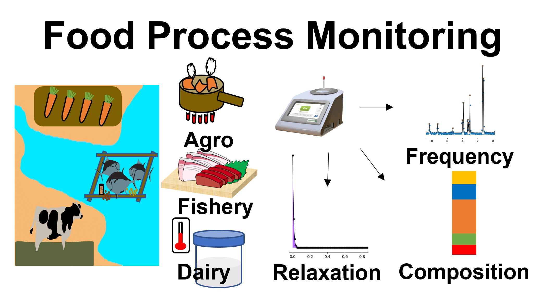
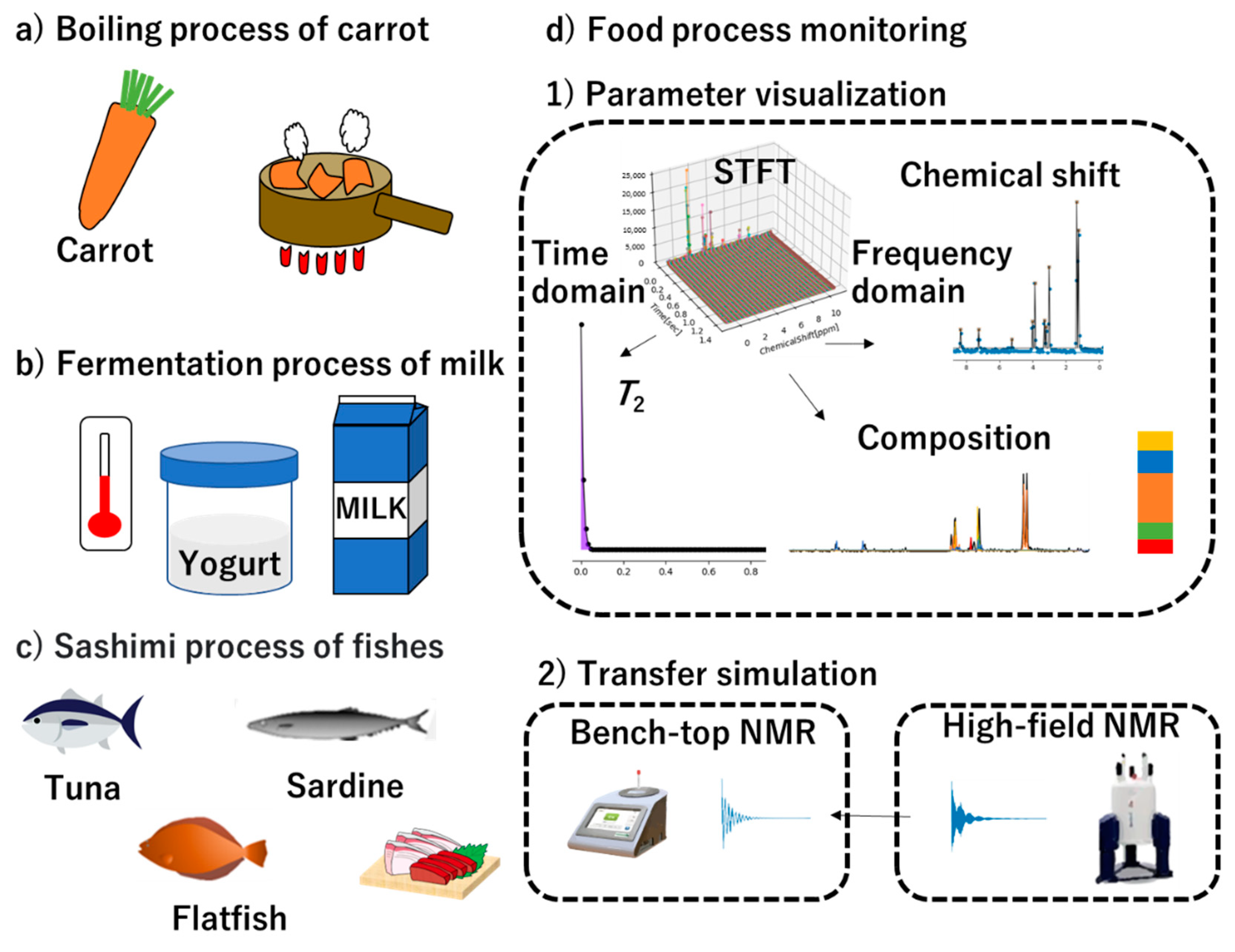
Parameter Visualization of Benchtop Nuclear Magnetic Resonance Spectra toward Food Process Monitoring

Abstract

Low-cost and user-friendly benchtop low-field nuclear magnetic resonance (NMR) spectrometers are typically used to monitor food processes in the food industry. Because of excessive spectral overlap, it is difficult to characterize food mixtures using low-field NMR spectroscopy. In addition, for standard compounds, low-field benchtop NMR data are typically unavailable compared to high-field NMR data, which have been accumulated and are reusable in public databases. This work focused on NMR parameter visualization of the chemical structure and mobility of mixtures and the use of high-field NMR data to analyze benchtop NMR data to characterize food process samples. We developed a tool to easily process benchtop NMR data and obtain chemical shifts and T₂ relaxation times of peaks, as well as transform high-field NMR data into low-field NMR data. Line broadening and time–frequency analysis methods were adopted for data processing. This tool can visualize NMR parameters to characterize changes in the components and mobilities of food process samples using benchtop NMR data. In addition, assignment errors were smaller when the spectra of standard compounds were identified by transferring the high-field NMR data to low-field NMR data rather than directly using experimentally obtained low-field NMR spectra.

1. Introduction

The sensitivity and resolution of an analytical nuclear magnetic resonance (NMR) spectrometer are significantly related to its magnetic field strength. Thus, state-of-the-art high-field NMR spectrometers that achieve field strength of up to 1200 MHz using superconductors have been developed [1]. However, a high-field NMR spectrometer has high initial investment, running, and maintenance costs [2]. Therefore, such spectrometers are expensive for small to medium-sized companies, government agencies, and public institutions, including those operating in primary agriculture, forestry, fishery sites, and food and chemical industries. Therefore, affordable low-field benchtop NMR spectrometers have been developed. These spectrometers are typically equipped with permanent magnets (42–100 MHz), which do not require expensive cooling systems and consumables [3]. Furthermore, these spectrometers require a smaller footprint than high-field NMR spectrometers; thus, they are easier to operate, and their operational costs are typically 1/5–1/20 of high-field spectrometers [3,4]. Benchtop low-field NMR spectrometers are widely used in different fields, such as agriculture, food chemistry, geology, pharmaceuticals, and materials science [5,6,7,8,9,10,11,12]. In recent years, we developed a database and performed statistical multivariate analyses such as nonnegative matrix factorization [13,14] for separating small and large molecules using a benchtop low-field NMR spectrometer. The focus of our applications is on the accumulation of NMR spectra of samples, which are obtained from a variety of food processes [15,16].

The low sensitivity and resolution of low-field NMR spectrometers [4,12] overlap NMR peaks, making NMR spectra difficult to analyze [3,17]. Furthermore, benchtop low-field NMR poses challenges in terms of sample throughput and measurement accuracy in the food industry [18]. Therefore, computational methods [19,20] and data-driven analyses [21,22] have been commonly used to improve low-field NMR spectra. The application of a computational method enables the extrapolation of information hidden in experimental data. Moreover, the accumulation and use of extrapolated information typically significantly reduces the amount of time and effort required for the measurements.

Various computational methods have been developed, including nmrglue [23], SIMPSON [24], SPINEVOLUTION [25], dmfit [26], EASY-GOING deconvolution [27], INFOS [28], Fityk [29], ssNake [30], spectral correction [31], spectral separation [32], fitting [33], numerical simulation [34], and noise reduction methods via principal component analysis [35]. During the analysis of low-field NMR spectra with extensive peak overlapping, sufficient data processing must be performed before the fitting process because of the dependence on the spectral phase, baseline, and signal-to-noise ratio (SNR) [31]. Moreover, spectral separation by fitting can determine the intensity, chemical shift, line width, and T₂* relaxation time of the peaks measured [35]. The simulation and fitting of low-field NMR spectra have generally been performed in either the frequency or time domain. We previously proposed a time–frequency analysis method, which is a signal deconvolution method that combines short-time Fourier transform (STFT) with probabilistic sparse matrix factorization [36] and nonnegative tensor/matrix factorization [22]. By simulating signals for both the frequency and time domains, we could separate signals related to the motility characteristics of the domain structure on the basis of chemical shift and T₂* relaxation time indicators in NMR spectra.

In principle, the T₂ relaxation time is the decay constant of a free-induced decay (FID), which is obtained by decaying the transverse magnetization resulting from the application of a 90° pulse. This study dealt with T₂*, which includes magnetic field inhomogeneity. The analysis of the FID relaxation time of a sample can provide important insights into the sample’s chemical composition, structure, and mobility [37,38]. The FID relaxation times can be calculated using Lorentzian, Gaussian, Voigt, and other functions in the frequency domain and the T₂* relaxation time equation in the time domain during the simulation and fitting of NMR signals [39,40]. The differences in T₂* relaxation times can be adjusted using the Weibull coefficient [37].

Spectral data transfer that adapts information about an acquired spectrum to the target spectrum is used when using data from different instruments [41]. Various methods were proposed for spectral data transfer from low-field to high-field NMR, which include direct standardization and piecewise direct standardization [42,43]. The possibility of NMR data transfer from a low field to a high field has also been investigated in time-domain NMR [44]. In addition, calibration transfer of low-field proton NMR (¹H-NMR) spectra using partial least squares regression in 40-, 60-, and 80-MHz benchtop NMR has been investigated [45].

In this study, we propose an approach that combines STFT fitting and data transfer simulations for food mixtures, which are analyzed using benchtop low-field NMR spectrometers. We note that the use of STFT fitting leading to NMR data transfer from high-field to low-field NMR has not been reported. We investigated the application of the proposed method to food process samples (boiling of carrot, fermentation of yogurt, and sashimi (raw fish)) characterized using low-field NMR spectrometers in a previous study [15]. First, we developed a parameter visualization tool to process benchtop NMR data and easily obtain chemical shifts and T₂ relaxation times of peaks. Second, we transformed high-field NMR data for standard compounds, which have been accumulated in public databases over many years, into low-field NMR data. Assignment and root-mean-square deviation (RMSD) values [46] were calculated for three fish food mixtures using spectral data measured using a 60 MHz benchtop low-field NMR spectrometer and simulated spectra transferred from 700 MHz NMR. Furthermore, the proposed method was applied to the evaluation of compositional changes in the milk fermentation process using 60-MHz NMR spectra. The results obtained using our method were then compared with previously reported simulated NMR spectra obtained using GISSMO [19].

2. Materials and Methods

2.1. NMR Measurements

High- and low-field NMR measurements were conducted using the AVANCE II-700 spectrometer (Bruker, Billerica, MA, USA) and benchtop NMReady-60PRO spectrometer (Nanalysis, Calgary, AB, Canada), respectively. ¹H-NMR measurements were conducted using both spectrometers. In the high-field NMR measurements, 65,536 data points were collected with a spectral width, relaxation time, dummy scans, and integration times of 16 ppm, 3 s, 4, and 32 s, respectively. In the low-field NMR measurements, 2048 data points with a spectral width of 12 ppm and a relaxation time of 3 s were obtained from previously measured food process monitoring data collected from primary industries such as agriculture (boiling process (0, 10, 30, 60 min) of carrot), dairy farming (fermentation process (0, 1.5, 3, 6, 8.5, 20, 24, 48 h) of milk), and fisheries (sashimi (raw fish) process of tuna (n = 2), sardine (n = 2), and flatfish (n = 1)) [15].

2.2. Data Processing and Parameter Visualization

The measured FIDs obtained using the high- and low-field NMR spectrometers were processed using nmrglue and the Python library. In particular, zero-filling, phase correction, baseline correction, and line broadening with a window function were performed (Figure S1). The processed FID data were then subjected to STFT to generate three-dimensional (3D) data with frequency/time/intensity information (Figures S2–S4). Data processing and parameter visualization (chemical shifts and T₂ relaxation times of peaks) results are output to a CSV file and images. By STFT, frequency information may be lost if the number of data points is small. The number of data points was adjusted to compensate for that frequency information.

2.3. Fitting Method

For the STFT-processed 3D data, a fitting method was used to identify and quantify the ingredients in a food sample. To fit frequency information, we used the Lorentz function [47,48], which is given by Equation (1).

$$L\left(x\right)=M_0\left(\frac{\gamma }{\pi \left(x^2+{\gamma }^2\right)}\right).$$

(1)

where $M_0$ represent intensities, $\gamma$ is the half-width at half-maximum in the Lorentzian function, and $x$ is the frequency information.

To fit temporal information, we used the T₂* relaxation time function [49] given by Equation (2).

$$M\left(t\right)=M_0^{\prime }exp\left\{-\left(\frac{t}{T_2^{*}}\right)\right\},$$

(2)

where $M_0^{\prime }$ represent intensities, $T_2^{*}$ represents the T₂* relaxation time, and $t$ is the time information.

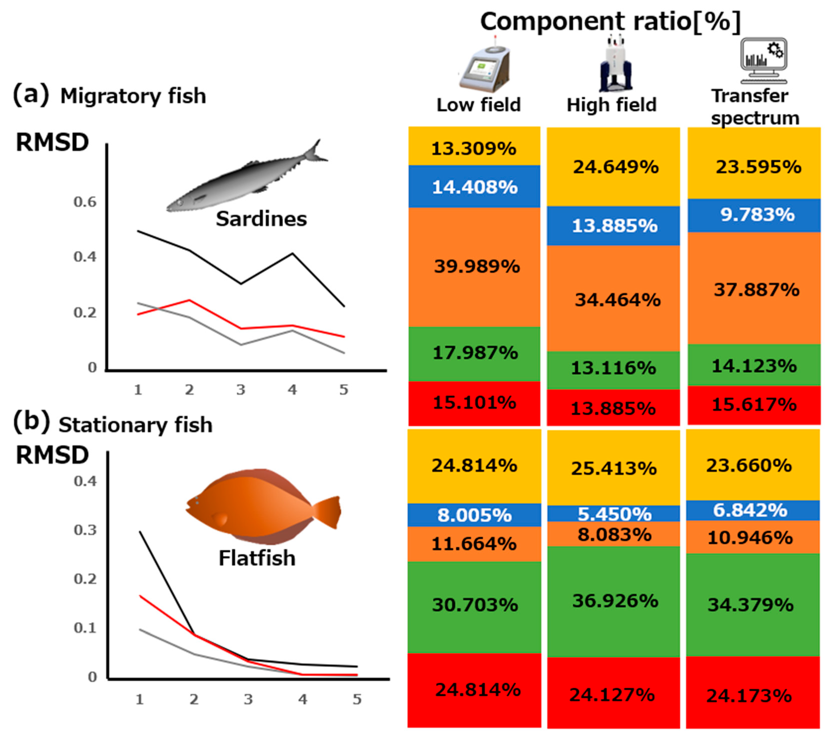
2.4. Identification of Components in Food Mixtures

Spectra of food process samples such as carrot, yogurt, and fish were annotated with reference to GISSMO [19] (Tables S1–S3). Data obtained from five standard compounds, including choline, trimethylamine N-oxide (TMAO), lactate, creatine, and histidine, as components based on previous analyses of fish and yogurt were obtained by fitting (see Table S4) [13,15,32]. Data obtained from tuna, sardine, and flatfish food mixtures were used for the characterization (see Tables S5–S7).

2.5. Removal of Water-Derived Spectra

Peaks within the range of 5.507–5.86 ppm were water-derived by low-field NMR. The calculation process was performed so that the peak intensities in this range were the same.

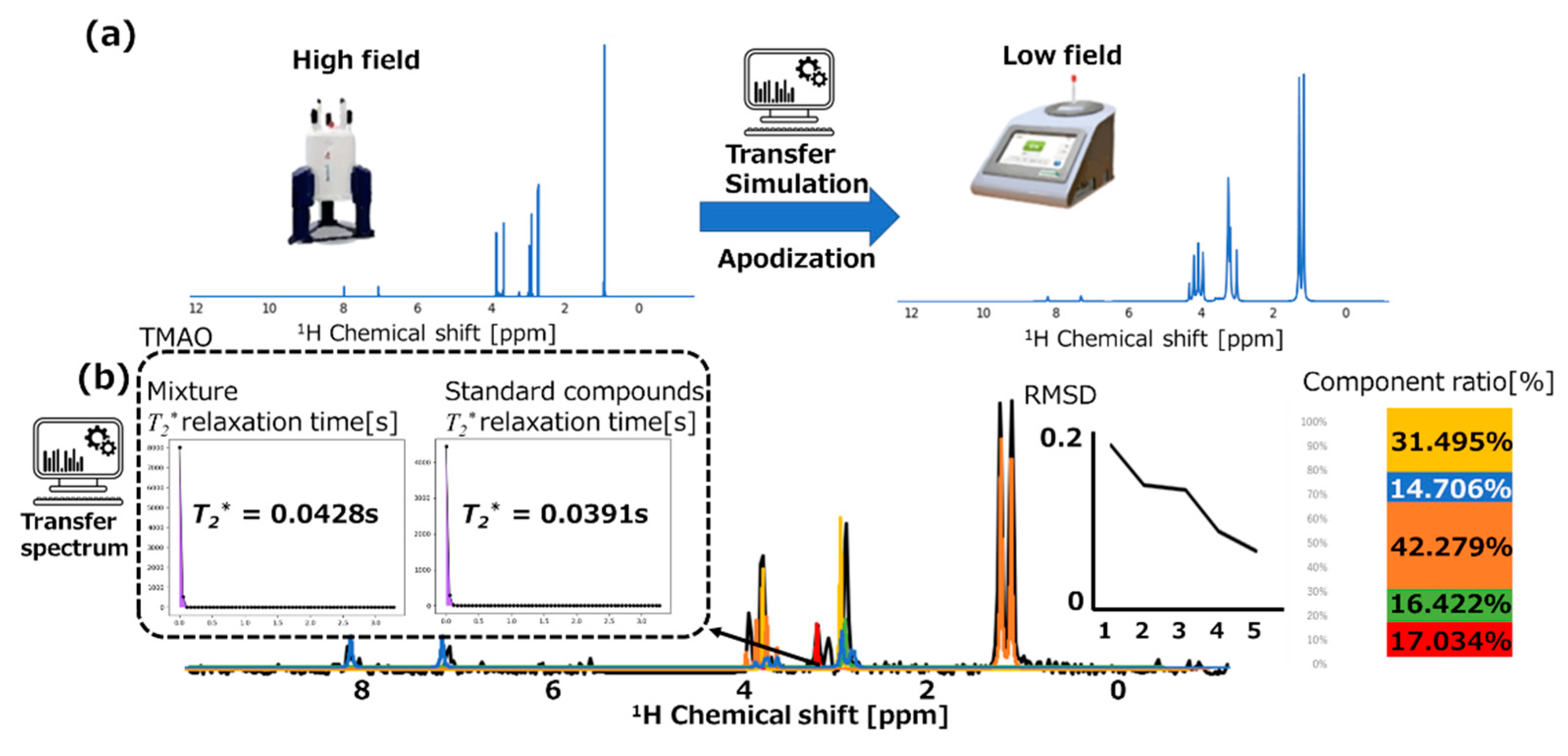
2.6. Transfer Simulation Method of NMR Data from High-Field to Low-Field NMR

An NMR data transfer simulation method was used to identify the peaks of benchtop NMR spectra with the reuse and transformation of high-field NMR spectra in the food mixtures. To account for errors in the spectral chemical shifts, we adjusted the ±0.03-ppm spectra by referring to previous studies [50]. In addition, we adjusted the pH of histidine in the standard compounds to reduce the RMSD value. The line broadening method [51], which integrates the window function of the exponential function into the spectrum, was used to convert high-field NMR data to low-field NMR data. The broadening parameter was 1 Hz, which was derived from a spectral width of 1.0 Hz ((11,600 Hz) × 0.0000896).

3. Results and Discussion

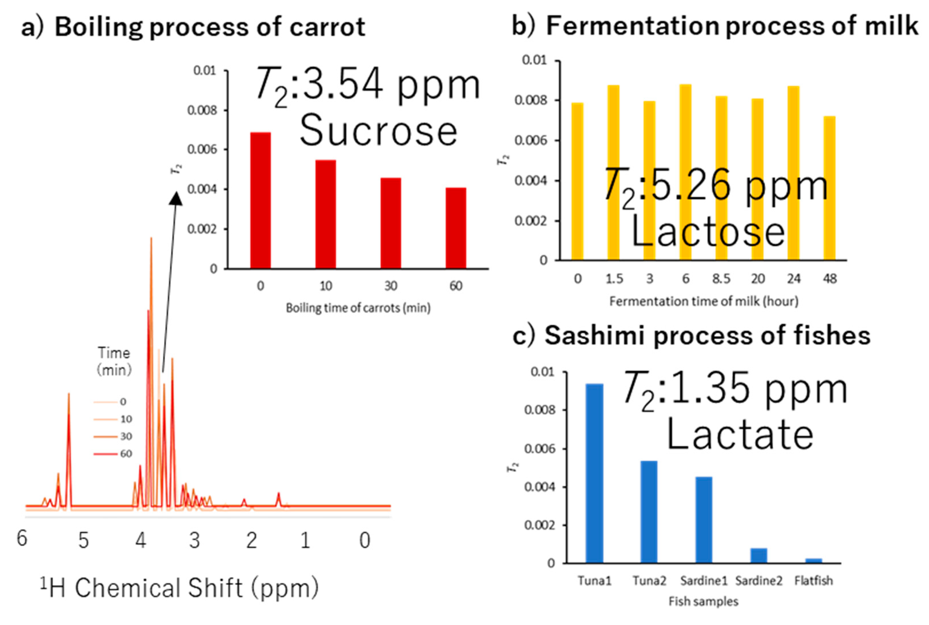
3.1. Parameter Visualization and Fitting

In our previous study, food processes, such as boiling carrots and fermentation of yogurt and sashimi raw fish, contain both small and large molecules, which produce broad NMR spectrum peaks [13,14,52]. Their components and physical properties change during food processes. In this study, we investigated methods and tools for parameter visualization and characterization of the components and the physical properties of mixtures in the food process (Figure 1a–c). The parameter visualization and transfer of NMR spectra from high-field to low-field NMR for NMR spectral characterization of compounds in food process samples in agriculture (a; boiling process of carrots), livestock (b; fermentation process of milk), and fishery (c; sashimi process of fishes) is summarized in Figure 1. The output of the parameter visualization process in tuna’s ¹H NMR data are shown in Figure S1. NMR data are processed as follows. (1) original FID, (2) zero-filling, (3) Fourier transform, (4) autophase correction, (5) manual phase correction, (6) autophase correction after manual phase correction, (7) baseline correction, (8) inverse Fourier transform, (9) water signal deletion and z-score calculation, (10) inverse Fourier transform after water signal deletion, (11) window function processing, (12) STFT, (13) visualization of the frequency domain of STFT-processed data, (14) z-score calculation and peak detection, (15) fitting of the frequency domain, and (16) visualization of peaks in the time domain.

Parameter visualization of ¹H NMR spectra involved in primary industry processes can provide information about the chemical shift and T² relaxation time for food process monitoring (Figure 2 and Figure S2). In the boiling process of carrots, the T₂ relaxation time of sucrose changes with the boiling time (Figure 2a, Figure S2a and Table S1). Thus, we could monitor the differences in the motility of carrot sucrose (3.54 ppm) due to heating. In the fermentation process of milk, there were no differences in the T₂ relaxation time of lactose (5.26 ppm) with fermentation time (Figure 2b, Figure S2b and Table S2). Thus, the components and conditions of the fermentation process can be monitored. In the sashimi process, differences in the T₂ relaxation time of lactate (1.35 ppm) were observed among different fish species and individuals (Figure 2c, Figure S2c and Table S3). Therefore, differences in composition and meat quality among fish species and individuals could be used for monitoring.

We performed STFT on both high-field and low-field NMR data of five standard compounds and a food mixture (i.e., tuna) to generate a set of 3D data with time/frequency information (Figures S3 and S4). The chemical shifts, intensities, and line widths of NMR peaks were obtained via peak picking and fitting to the frequency information contained in the generated 3D data. The T₂* relaxation time was obtained by fitting the time information. The parameters for the sample compounds and food mixture (i.e., tuna, sardine, and flatfish) tested are summarized in Tables S4–S6, respectively. The amounts of the five standard compounds found in the food mixture were calculated via low-field NMR spectroscopy (Figure 3a). The two peaks in the food mixture (black curve) shifted significantly from the histidine assignment of the standard compound to the low-field NMR data (blue curve). This could be due to the difference in pH between the food mixture and sample compounds. The shifts observed for the lactate peaks (orange curve) were also similar. A representative T₂* relaxation time at an FID of approximately 4.5 ppm in the 3D data was calculated. The T₂* relaxation times for TMAO in the food mixture and its standard compound were 0.0428 and 0.0342 s, respectively. When the number of included standards was five, the RMSD value that evaluates the difference between the mixture and the set of standards was 0.191. Lactate was the most abundant component, followed by histidine, creatine, choline, and TMAO.

The same food mixture and standard compounds were also analyzed by high-field NMR spectroscopy. The content of each standard compound in the food mixture was calculated similarly (Figure 3b). The assignment of histidine in the high-field NMR data (blue curve) demonstrated that the two peaks in the food mixture (black curve) shifted similarly compared to the low-field NMR data (Figure 3a). The calculated representative T₂* relaxation times for TMAO in the food mixture and its standard compound were 0.226 and 0.120 s, respectively. When the number of included standards was 5, the RMSD value was 0.210. Interestingly, the amounts of the components found followed the order of lactate, creatine, histidine, choline, and TMAO.

We observed a difference in the creatine content between the low-field and high-field NMR spectra, which are shown on the right side of Figure 3a,b, respectively. This was primarily due to the smaller SNR in the low-field NMR spectra because their RMSD values were lower than those in the high-field NMR spectra. The higher the SNR values in the high-field NMR spectra, the lower the errors; therefore, transforming this feature into low-field NMR spectra will be beneficial. Meanwhile, the T₂* relaxation time was longer in the high-field NMR data.

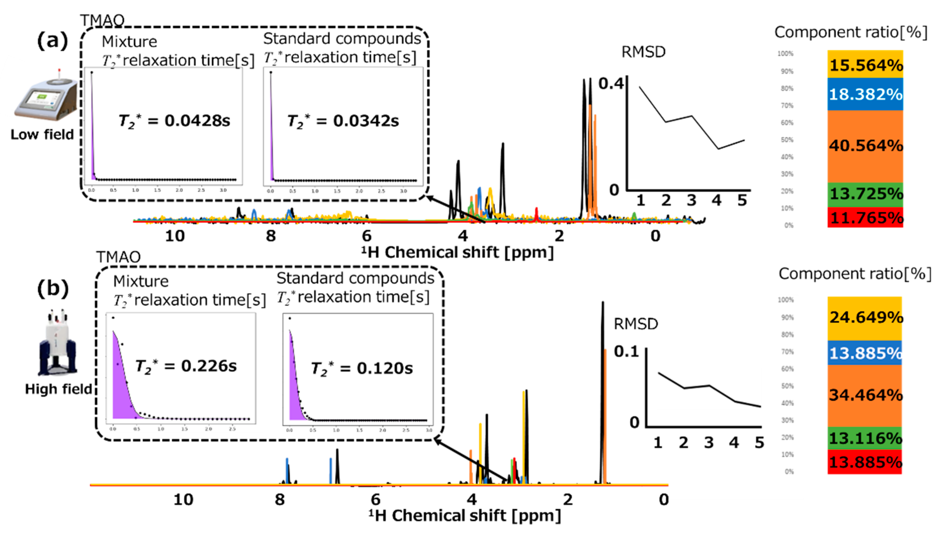
3.2. Transfer Simulation of NMR Data Transfer from High-Field to Low-Field

We simulated NMR data transfer from high-field to low-field and assigned the transferred data to food mixture spectra in low-field NMR. The transfer of 700-MHz NMR data for the standard compounds to 60-MHz data are depicted in Figure 4a. The results of assigning the five standard compounds to the low-field NMR spectrum for the food mixture (i.e., tuna) via data transfer simulation are summarized in Figure 4b. The RMSD value shown in Figure 4b (center) is increased by 42% compared with the low-field value shown in Figure 3a (center). The creatine content shown in Figure 4b (right) is close to the observed high-field data shown in Figure 3b (right). Therefore, the proposed transfer of high SNR in high-field NMR to low-field NMR data could be useful for improving the assignment of low-field NMR spectra.

We extended our approach of transfer simulations to two sashimi (raw fish) food mixtures, including migratory (i.e., sardine) and stationary (i.e., flatfish) fishes (Figure 5). The contents of the same compounds were calculated because these compounds were also found in the additional samples. The results for the sardine and flatfish samples are depicted in Figure 5a,b, respectively. We note that both tuna and sardine are migratory fishes. A high level of lactate was found in the sardine sample, as in the case of the tuna sample (Figure 4b). Meanwhile, a high level of TMAO was detected in the flatfish sample, which agreed with our previous finding that TMAO as a compatible solute is abundant in stationary fishes [13]. In addition, the amount of histidine found in the flatfish sample was lower than that in the tuna and sardine samples. This result implied that the histidine content increased because of pH buffering by lactate [49]. In addition, our findings enabled us to detect the differences in the content ratios of the targeted compounds among fish species.

The RMSD values for the tested sardine sample for the low-field (Figure 5a, left, black line), high-field (Figure 5a, left, red line), and transfer spectra (Figure 5a, left, gray line) were 0.208, 0.156, and 0.0810, respectively. For the flatfish sample, the values were 0.00301, 0.00132, and 0.00101, respectively (Figure 5b, left). These results implied improvements in the low-field NMR analyses applying the proposed transfer simulation method to high-field NMR. A possible reason for the larger RMSD value in (a) was the effect of pH in vivo. We have previously observed chemical shifts caused by the pH differences in the high-field NMR data of standard compounds [46]. In this study, we focused on histidine, which showed large differences in chemical shift between the spectra of food mixtures and sample compounds. We found significant chemical shifts in the data obtained from different pH values (e.g., Figure S5) against each standard compound. The use of experimental optimization will probably increase the RMSD values, therefore improving the proposed transfer simulation method.

We also successfully performed the transfer of transferred 60-MHz NMR spectra of the milk fermentation process by introducing yogurt samples (Figure S6), suggesting that the proposed method can be used to evaluate other foods and their changes. There is still room for technological development regarding the handling of multiplets in the proposed method, and this is an issue for future study. The proposed method is limited to singlets or very simple multiples. However, for reliable spectral transfer to low fields, more complex multiplet simulations must be performed; GISSMO simulations can generate high-field NMR data with good peak separation and simulate “ideal” low-field NMR data (Figure S7). Therefore, GISSMO can be used to generate spectra from singlet to multiplets. In future studies, we aim to apply the proposed method to components, such as meat, food-derived proteins, and plastics, which generate more complex spectra.

4. Conclusions

We developed a tool for parameter visualization and simulation for transferring high-field NMR data to low-field NMR to characterize the chemical structures and mobilities of mixtures in food processes, which were analyzed using a benchtop low-field NMR spectrometer. This tool can easily obtain chemical shifts and T₂ relaxation times of peaks from benchtop NMR data. In addition, the results demonstrated the feasibility of the data transfer despite the significantly different dispersion (separation) of peaks between high-field and low-field NMR spectrometers. In addition, the assignment errors were smaller when the spectra of standard compounds were identified by transferring high-field NMR data rather than directly using the experimentally obtained low-field NMR spectra. These findings will likely promote digitization and monitoring in food processing industries, where low-cost benchtop low-field NMR data can be analyzed by reusing NMR spectral data acquired with expensive high-field NMR data.

References

1. Callon, M.; Malär, A.A.; Pfister, S.; Římal, V.; Weber, M.E.; Wiegand, T.; Zehnder, J.; Chávez, M.; Cadalbert, R.; Deb, R.; et al. Biomolecular solid-state NMR spectroscopy at 1200 MHz: The gain in resolution. J. Biomol. Nmr 2021, 75, 255–272. [Google Scholar] [CrossRef] [PubMed]
2. Gunning, Y.; Taous, F.; El Ghali, T.; Gibbon, J.D.; Wilson, E.; Brignall, R.M.; Kemsley, E.K. Mitigating instrument effects in 60 MHz 1H NMR spectroscopy for authenticity screening of edible oils. Food Chem. 2022, 370, 131333. [Google Scholar] [CrossRef] [PubMed]
3. Grootveld, M.; Percival, B.; Gibson, M.; Osman, Y.; Edgar, M.; Molinari, M.; Mather, M.L.; Casanova, F.; Wilson, P.B. Pro-Gress in low-field benchtop NMR spectroscopy in chemical and biochemical analysis. Anal. Chim. Acta 2019, 1067, 11–30. [Google Scholar] [CrossRef] [Green Version]
4. Van Beek, T.A. Low-field benchtop NMR spectroscopy: Status and prospects in natural product analysis†. Phytochem. Anal. 2021, 32, 24–37. [Google Scholar] [CrossRef] [Green Version]
5. Hu, X.Y.; Wu, P.; Zhang, S.P.; Chen, S.; Wang, L. Moisture conversion and migration in single-wheat kernel during iso-thermal drying process by LF-NMR. Drying Technol. 2019, 37, 803–812. [Google Scholar] [CrossRef]
6. Kirtil, E.; Oztop, M.H. 1H nuclear magnetic resonance relaxometry and magnetic resonance imaging and applications in food science and processing. Food Eng. Rev. 2016, 8, 1–22. [Google Scholar] [CrossRef]
7. Zhang, Q.; Liang, F.; Pang, Z.L.; Jiang, S.; Zhou, S.W.; Zhang, J.C. Lower threshold of pore-throat diameter for the shale gas reservoir: Experimental and molecular simulation study. J. Petrol. Sci. Eng. 2019, 173, 1037–1046. [Google Scholar] [CrossRef]
8. Metz, H.; Mäder, K. Benchtop-NMR and MRI—A new analytical tool in drug delivery research. Int. J. Pharm. 2008, 364, 170–175. [Google Scholar] [CrossRef]
9. Zhao, H.T.; Wu, X.; Huang, Y.Y.; Zhang, P.; Tian, Q.; Liu, J.P. Investigation of moisture transport in cement-based materials using low-field nuclear magnetic resonance imaging. Mag. Concr. Res. 2021, 73, 252–270. [Google Scholar] [CrossRef]
10. Blümich, B.; Singh, K. Desktop NMR and its applications from materials science to organic chemistry. Angew. Chem. Int. Ed. Engl. 2018, 57, 6996–7010. [Google Scholar] [CrossRef]
11. Blümich, B. Low-field and benchtop NMR. J. Magn. Reson. 2019, 306, 27–35. [Google Scholar] [CrossRef] [PubMed]
12. Ates, E.G.; Domenici, V.; Florek-Wojciechowska, M.; Gradišek, A.; Kruk, D.; Maltar-Strmečki, N.; Oztop, M.; Ozvural, E.B.; Rollet, A.L. Field-dependent NMR relaxometry for food science: Applications and perspectives. Trends Food Sci. Technol. 2021, 110, 513–524. [Google Scholar] [CrossRef]
13. Wei, F.; Fukuchi, M.; Ito, K.; Sakata, K.; Asakura, T.; Date, Y.; Kikuchi, J. Fish ecotyping based on machine learning and inferred network analysis of chemical and physical properties. Sci. Rep. 2021, 11, 2766. [Google Scholar] [CrossRef] [PubMed]
14. Wei, F.; Fukuchi, M.; Ito, K.; Sakata, K.; Asakura, T.; Date, Y.; Kikuchi, J. Large-scale evaluation of major soluble macromo-lecular components of fish muscle from conventional 1H NMR spectral database. Molecules 2020, 25, 1966. [Google Scholar] [CrossRef] [Green Version]
15. Chikayama, E.; Yamashina, R.; Komatsu, K.; Tsuboi, Y.; Sakata, K.; Kikuchi, J.; Sekiyama, Y. FoodPro: A web-based tool for evaluating covariance and correlation NMR spectra associated with food processes. Metabolites 2016, 6, 36. [Google Scholar] [CrossRef] [Green Version]
16. Kikuchi, J.; Yamada, S. The exposome paradigm to predict environmental health in terms of systemic homeostasis and re-source balance based on NMR data science. RSC Adv. 2021, 11, 30426–30447. [Google Scholar] [CrossRef]
17. Fechete, R.; Morar, I.A.; Moldovan, D.; Chelcea, R.I.; Crainic, R.; Nicoară, S.C. Fourier and Laplace-like low-field NMR spectroscopy: The perspectives of multivariate and artificial neural networks analyses. J. Magn. Reson. 2021, 324, 106915. [Google Scholar] [CrossRef]
18. Ezeanaka, M.C.; Nsor-Atindana, J.; Zhang, M. Online low-field nuclear magnetic resonance (LF-NMR) and magnetic reso-nance imaging (MRI) for food quality optimization in food processing. Food Bioprocess Technol. 2019, 12, 1435–1451. [Google Scholar] [CrossRef]
19. Dashti, H.; Westler, W.M.; Tonelli, M.; Wedell, J.R.; Markley, J.L.; Eghbalnia, H.R. Spin system modeling of nuclear magnetic resonance spectra for applications in metabolomics and small molecule screening. Anal. Chem. 2017, 89, 12201–12208. [Google Scholar] [CrossRef]
20. Dashti, H.; Wedell, J.R.; Westler, W.M.; Tonelli, M.; Aceti, D.; Amarasinghe, G.K.; Markley, J.L.; Eghbalnia, H.R. Applications of parametrized NMR spin systems of small molecules. Anal. Chem. 2018, 90, 10646–10649. [Google Scholar] [CrossRef] [Green Version]
21. Ito, K.; Xu, X.; Kikuchi, J. Improved prediction of carbonless NMR spectra by the machine learning of theoretical and fragment descriptors for environmental mixture analysis. Anal. Chem. 2021, 93, 6901–6906. [Google Scholar] [CrossRef] [PubMed]
22. Yamada, S.; Chikayama, E.; Kikuchi, J. Signal deconvolution and generative topographic mapping regression for solid-state NMR of multi-component materials. Int. J. Mol. Sci. 2021, 22, 1086. [Google Scholar] [CrossRef] [PubMed]
23. Helmus, J.J.; Jaroniec, C.P. Nmrglue: An open source Python package for the analysis of multidimensional NMR data. J. Biomol. Nmr 2013, 55, 355–367. [Google Scholar] [CrossRef] [PubMed] [Green Version]
24. Bak, M.; Rasmussen, J.T.; Nielsen, N.C. Simpson: A general simulation program for solid-state NMR spectroscopy. J. Magn. Reson. 2000, 147, 296–330. [Google Scholar] [CrossRef] [Green Version]
25. Veshtort, M.; Griffin, R.G. SPINEVOLUTION: A powerful tool for the simulation of solid and liquid state NMR experiments. J. Magn. Reson. 2006, 178, 248–282. [Google Scholar] [CrossRef]
26. Massiot, D.; Fayon, F.; Capron, M.; King, I.; Le Calvé, S.; Alonso, B.; Durand, J.; Bujoli, B.; Gan, Z.; Hoatson, G. Modelling one- and two-dimensional solid-state NMR spectra. Magn. Reson. Chem. 2002, 40, 70–76. [Google Scholar] [CrossRef]
27. Grimminck, D.L.; van Meerten, B.; Verkuijlen, M.H.; van Eck, E.R.; Meerts, W.L.; Kentgens, A.P. EASY-GOING deconvolution: Automated MQMAS NMR spectrum analysis based on a model with analytical crystallite excitation efficiencies. J. Magn. Reson. 2013, 228, 116–124. [Google Scholar] [CrossRef]
28. Smith, A.A. INFOS: Spectrum fitting software for NMR analysis. J. Biomol. NMR 2017, 67, 77–94. [Google Scholar] [CrossRef]
29. Schulze, H.G.; Rangan, S.; Vardaki, M.Z.; Blades, M.W.; Turner, R.F.B.; Piret, J.M. Critical evaluation of spectral resolution enhancement methods for Raman hyperspectra. Appl. Spectrosc. 2022, 76, 61–80. [Google Scholar] [CrossRef]
30. Van Meerten, S.G.J.; Franssen, W.M.J.; Kentgens, A.P.M. ssNake: A cross-platform open-source NMR data processing and fitting application. J. Magn. Reson. 2019, 301, 56–66. [Google Scholar] [CrossRef]
31. Matviychuk, Y.; Steimers, E.; von Harbou, E.; Holland, D.J. Improving the accuracy of model-based quantitative nuclear magnetic resonance. Magn. Reson. 2020, 1, 141–153. [Google Scholar] [CrossRef]
32. Yamada, S.; Ito, K.; Kurotani, A.; Yamada, Y.; Chikayama, E.; Kikuchi, J. InterSpin: Integrated supportive Webtools for low- and high-field NMR analyses toward molecular complexity. ACS Omega 2019, 4, 3361–3369. [Google Scholar] [CrossRef] [PubMed]
33. Schneider, H.; Saalwächter, K.; Roos, M. Complex morphology of the intermediate phase in block copolymers and semicrystalline polymers as revealed by H-1 NMR spin diffusion experiments. Macromolecules 2017, 50, 8598–8610. [Google Scholar] [CrossRef]
34. Kurz, R.; Schulz, M.; Scheliga, F.; Men, Y.F.; Seidlitz, A.; Thurn-Albrecht, T.; Saalwächter, K. Interplay between crystallization and entanglements in the amorphous phase of the crystal-fixed polymer poly(ε-caprolactone). Macromolecules 2018, 51, 5831–5841. [Google Scholar] [CrossRef]
35. Kusaka, Y.; Hasegawa, T.; Kaji, H. Noise reduction in solid-state NMR spectra using principal component analysis. J. Phys. Chem. A 2019, 123, 10333–10338. [Google Scholar] [CrossRef]
36. Yamada, S.; Kurotani, A.; Chikayama, E.; Kikuchi, J. Signal deconvolution and noise factor analysis based on a combination of time-frequency analysis and probabilistic sparse matrix factorization. Int. J. Mol. Sci. 2020, 21, 2978. [Google Scholar] [CrossRef] [Green Version]
37. Borsacchi, S.; Sudhakaran, U.P.; Calucci, L.; Martini, F.; Carignani, E.; Messori, M.; Geppi, M. Rubber-filler interactions in polyisoprene filled with in situ generated silica: A solid state NMR study. Polymers 2018, 10, 822. [Google Scholar] [CrossRef] [Green Version]
38. Monaretto, T.; Moraes, T.B.; Colnago, L.A. Recent 1D and 2D TD-NMR pulse sequences for Plant Science. Plants 2021, 10, 833. [Google Scholar] [CrossRef]
39. Wang, F.F.; Deng, Z.; Yang, Z.J.; Sun, P.C. Heterogeneous dynamics and microdomain structure of high-performance chi-tosan film as revealed by solid-state NMR. J. Phys. Chem. C 2021, 125, 13572–13580. [Google Scholar] [CrossRef]
40. Rossini, A.J.; Widdifield, C.M.; Zagdoun, A.; Lelli, M.; Schwarzwälder, M.; Copéret, C.; Lesage, A.; Emsley, L. Dynamic nuclear polarization enhanced NMR spectroscopy for pharmaceutical formulations. J. Am. Chem. Soc. 2014, 136, 2324–2334. [Google Scholar] [CrossRef]
41. Workman, J.J. A review of calibration transfer practices and instrument differences in spectroscopy. Appl. Spectrosc. 2018, 72, 340–365. [Google Scholar] [CrossRef] [PubMed]
42. Monakhova, Y.B.; Diehl, B.W.K. A procedure for calibration transfer of DOSY NMR measurements: An example of molecular weight of heparin preparations. J. Chemom. 2020, 34, e3210. [Google Scholar] [CrossRef]
43. Monakhova, Y.B.; Diehl, B.W.K. Transfer of multivariate regression models between high-resolution NMR instruments: Application to authenticity control of sunflower lecithin. Magn. Reson. Chem. 2016, 54, 712–717. [Google Scholar] [CrossRef] [PubMed]
44. Hou, X.W.; Wang, X.; Hu, Y.; Chen, Y.; Huang, G.; Nie, S.D. A one-dimensional U-net-based calibration-transfer method for low-field nuclear magnetic resonance signals. Anal. Chem. 2021, 93, 10469–10476. [Google Scholar] [CrossRef] [PubMed]
45. Galvan, D.; Bona, E.; Borsato, D.; Danieli, E.; Montazzolli Killner, M.H.M. Calibration transfer of partial least squares regression models between desktop nuclear magnetic resonance spectrometers. Anal. Chem. 2020, 92, 12809–12816. [Google Scholar] [CrossRef] [PubMed]
46. Yamawaki, R.; Tei, A.; Ito, K.; Kikuchi, J. Decomposition factor analysis based on virtual experiments throughout bayesian optimization for compost-degradable polymers. Appl. Sci. 2021, 11, 2820. [Google Scholar] [CrossRef]
47. Bruce, S.D.; Higinbotham, J.; Marshall, I.; Beswick, P.H. An analytical derivation of a popular approximation of the Voigt function for quantification of NMR spectra. J. Magn. Reson. 2000, 142, 57–63. [Google Scholar] [CrossRef]
48. Sun, Y.C.; Xin, J. Lorentzian peak sharpening and sparse blind source separation for NMR spectroscopy. Signal Image Video Process 2022, 16, 633–641. [Google Scholar] [CrossRef]
49. Besghini, D.; Mauri, M.; Simonutti, R. Time domain NMR in polymer science: From the laboratory to the industry. Appl. Sci. 2019, 9, 1801. [Google Scholar] [CrossRef] [Green Version]
50. Chikayama, E.; Sekiyama, Y.; Okamoto, M.; Nakanishi, Y.; Tsuboi, Y.; Akiyama, K.; Saito, K.; Shinozaki, K.; Kikuchi, J. Statistical indices for simultaneous large-scale metabolite detections for a single NMR spectrum. Anal. Chem. 2010, 82, 1653–1658. [Google Scholar] [CrossRef]
51. Krafčík, D.; Ištvánková, E.; Džatko, Š.; Víšková, P.; Foldynová-Trantírková, S.; Trantírek, L. Towards profiling of the G-quadruplex targeting drugs in the living human cells using NMR spectroscopy. Int. J. Mol. Sci. 2021, 22, 6042. [Google Scholar] [CrossRef] [PubMed]
52. Asakura, T.; Date, Y.; Kikuchi, J. Application of ensemble deep neural network to metabolomics studies. Anal. Chim. Acta 2018, 1037, 230–236. [Google Scholar] [CrossRef] [PubMed]
Figure 1. Conceptual diagram of the proposed proton nuclear magnetic resonance (1H-NMR) spectral analysis using parameter visualization of benchtop NMR spectra toward food process monitoring. This study focused on food process monitoring in primary industries such as fishery, dairy farming, and agriculture. For example, food processes of the boiling status of carrot (a), the fermentation status of milk (b), and the quality of fish meats (c) were handled. (d1) For food process monitoring, a parameter visualization of NMR data is depicted. (d2) Conceptual diagram of transition simulation to use high magnetic field NMR data are shown.
Processes 10 01264 g001
Figure 2. Parameter visualization of 1H NMR spectra involved in primary industry processes. An example of parameter visualization about chemical shift and T2 for NMR datasets for fisheries, livestock, and agriculture is shown. (a) NMR dataset of the boiling process of carrots in agriculture. (b) NMR dataset of the fermentation process of milk in the livestock industry. (c) NMR dataset of sashimi process of fishes (tuna, sardine, and flatfish) in the fishery industry.
Processes 10 01264 g002
Figure 3. Assignment results and root-mean-square deviation values for standard compounds to food mixtures (tuna), which were measured through (a) low-field and (b) high-field NMR spectroscopy. The black curves represent the spectra of the food mixture. Red, green, orange, blue, and yellow represent the spectrum and component ratio of choline, trimethylamine N-oxide (TMAO), lactate, histidine, and creatine, respectively. Calculated representative T2* relaxation times are depicted for TMAO in the food mixture and its standard compound.
Processes 10 01264 g003
Figure 4. (a) High-field 1H-NMR spectra before and after the data transfer simulation. (b) Assignment results and root-mean-square deviation values of spectra for standard compounds, which were transferred to the corresponding compounds in the food mixtures (tuna) analyzed by benchtop low-field NMR. Red, green, orange, blue, and yellow represent the spectrum and component ratio of choline, TMAO, lactate, histidine, and creatine, respectively. Calculated representative T2* relaxation times are displayed for TMAO in the food mixture and its standard compound.
Processes 10 01264 g004
Figure 5. Contents of compounds obtained from low-field, high-field, and transferred NMR spectra in the two fish samples: (a) migratory (sardine) and (b) stationary (flatfish) fish samples. Component ratios are obtained (from left to right) by low-field NMR, high-field NMR, and transfer NMR simulated spectra. Red, green, orange, blue, and yellow represent the spectrum and component ratio of choline, TMAO, lactate, histidine, and creatine, respectively.
Processes 10 01264 g005
Publisher’s Note: MDPI stays neutral with regard to jurisdictional claims in published maps and institutional affiliations.