EOQ Models for Imperfect Items under Time Varying Demand Rate

Abstract

In the classical Economic Order Quantity (EOQ) model, the common unrealistic assumptions are that all the purchased items are of perfect quality and the demand is constant. However, in a real-world environment, a portion of the purchased items might be damaged due to mishandling or an accident during the shipment process, and the demand rate may increase or decrease over time. Many companies are torn between repairing or replacing the imperfect items with new ones. The right decision on that options is crucial in order to guarantee that there is no shortage of stocks while at the same time not jeopardising the items’ quality and maximising the company’s profit. This paper investigates two EOQ models for imperfect quality items by assuming the demand rate varies with time. Under Policy 1, imperfect items are sent for repairs at an additional cost to the makeup margin; under Policy 2, imperfect items are replaced with equivalent quality items from a local supplier at a higher price. Two mathematical models are developed, and numerical examples along with sensitivity analyses are provided to illustrate these models. Our results reveal that Policy 1 is preferable to Policy 2 most of the time. However, Policy 2 outperforms Policy 1 if there is no minimum threshold on the purchased stock quantity. This research allows a company to discover solutions to previously identified inventory problems and make the inventory-patching process more controlled.

1. Introduction

Academics and practitioners have demonstrated over the last few decades that effective inventory management is one of the essential predictors of a company’s performance in a challenging business environment. In general, the decision made by a company to maximise profit while satisfying demand depends significantly on the inventory models. The oldest classical inventory model is the Economic Order Quantity (EOQ). Based on this model, it is tacitly assumed that the received items are of perfect quality. However, in real-life applications, this assumption may not always be true. The received items may be damaged or spoiled due to negligence in process control, transit or handling processes. The existence of imperfect items should not be ignored because it enormously impacts the total cost of an inventory system. Due to this issue, many studies have recently focused on the inventory model considering imperfect quality items. A common assumption made by existing studies is that the imperfect items are revoked or withdrawn at the end of the product cycle and then sold at a discounted price. However, instead of offering a discounted price, the imperfect items can be substituted with new items purchased from another supplier or sent in for repair before the end of the cycle. These options can be selected based on the considerable value of the imperfect items. Perhaps it will assist the managers of a company in making the best decision while also satisfying the demand and minimising inventory costs.

The assumption of a constant demand rate over a finite planning horizon is another limitation of the classical EOQ model. It should be noted the supposition of a constant demand rate is only valid during the maturity phase of a product life cycle. In fact, patterns of time-varying demand reflect sales in different phases of a product life cycle. Hence, during the growth stage of a product life cycle, the demand rate should not be constant. For example, the demand rate for newly launched electronic products increases at the beginning of the cycle. The demand rate for these products will decrease when the product becomes obsolete or a better electronic product hits the market. The same applies to fashionable products such as clothes and cosmetics. The demand rate for these fashionable products will increase astonishingly during the early cycle and drop dramatically when the products become outdated. Furthermore, for seasonal inventory, the demand rate is either increasing or decreasing with time. Seasonal inventory refers to items that are in high or low demand at specific times of the year, i.e., the demand fluctuates throughout the year due to weather, seasons, events, celebration or holidays. This fluctuation in demand is reflected in orders/sales during those particular periods, and thus the management of stock level is a key in response to the waxing and waning of demand. Hence, inventory models with time-varying demand should be considered. Indeed, the demand rate should be represented by a continuous linear or quadratic function of time [1].

Motivated by the aforementioned issues, this paper aims to develop two inventory models that consider imperfect items under time-varying demand rates. Specifically, our focus is on these two policies:

• Policy 1: Sending the imperfect items for repair.
• Policy 2: Purchasing new items from another supplier to replace the imperfect items.

We note here that Jaber et al. [2] considered the above two policies under the assumption of a constant demand rate. As previously stated, a constant demand rate is only valid throughout the maturity phase of a product life cycle. Therefore, the work of Jaber et al. [2] has covered the maturity phase of a product life cycle. This paper will consider the growth stage of a product life cycle where the demand rate is assumed to be linear. The rest of this paper is organised as follows. Section 2 highlights the relevant literature, followed by the listing of notations and assumptions in Section 3. Section 4 provides the mathematical formulation of the two models. By using the derived mathematical formulation, numerical examples and sensitivity analyses are carried out and discussed in Section 5. Finally, Section 7 concludes with key findings and suggests ideas for future research.

2. Literature Review

A typical assumption made by most existing researchers in the EOQ model is that all of the items produced by the facility are of perfect quality. Multiple suggestions are provided in later works to deal with this unrealistic assumption, where the supposition of all perfect-quality items is no longer considered, i.e., the necessity for all items to be ideal throughout the process is removed, matching the real-life scenarios. In reality, imperfect items do exist, and these could be factory-defective items or damaged items due to transportation or handling processes. Many researchers began their work by assuming that imperfect items are withdrawn from inventory as a single batch, either at the end of the screening period or at the end of the cycle. The imperfect items are then sold at a discounted price. Furthermore, other researchers have considered the possibility in which errors are committed during the screening for defective items, either by the manufacturer (as in Yoo et al. [3]) or by the buyer (as in Khan et al. [4,5], Dey and Giri [6]). It is worth mentioning the extension study of Hsu and Hsu [7] by Khalilpourazari et al. [8], where they proposed a multi-item EOQ model with the presence of imperfect products in supply deliveries. Their inspection process is subject to committing Type-I or Type-II errors, and operational constraints such as warehouse capacity and budget are set to establish a more applicable model. In a few words, all goods must be inspected before defective items can be identified. Al-Salamah [9,10], Bose and Guha [11], Cheikhrouhou et al. [12], Chen and Tsai [13], Genta et al. [14], Ouyang et al. [15], among others, have also contributed to the inventory system with inspection of items under various realistic assumptions. Some of these papers, however, considered inspection but not inspection errors.

Salameh and Jaber [16] developed the EOQ model where a shipment contains a random fraction of defective items. When the stocks are received, they assume that the stocks are screened immediately to ensure that there are no shortages. They classified the items that did not pass the screening process as “imperfect” and considered them as second-grade products instead of eliminating them directly from the inventory altogether. Then, they constructed a model that assumes that the imperfect items are sold at a discounted price as lower-quality products. However, there are always better alternatives to cope with the issue of defective items, and the subsequent extension for this realistic problem induces more economical solutions.

The works by Salameh and Jaber [16] were then improvised by Jaber et al. [2]. Their paper replaced the alternative of selling imperfect items at lower costs with two options. For the first option, the imperfect items are replaced by purchasing the same number of items from a local supplier but at a higher cost, whereas for the second option, the imperfect items are sent for repairs and restorations at a third-party facility and are eventually returned to the inventory. The rationale behind the first option is that an emergency shipment from a distant supplier to substitute the defective items may not be feasible.

The literature above explores the models under a constant demand rate assumption. Nevertheless, in reality, the demand rate of an item is not always constant, as it is subject to variations due to climate conditions, price, income, style, taste and population, to mention but a few. All these variables can cause an impactful variation in the demand for items. The assumption that the demand rate is constant is only valid throughout the maturity phase of a product life cycle (see [17]). Sometimes a product may experience a surge in demand even during its maturity phase. For example, gloves and masks became household essentials during the COVID-19 pandemic [18]. In Example 2 in [17], Dye and Hsieh considered products during the growth phase of their product life cycle, and they assumed that the time-varying demand rate is linearly increasing. The demand for trendy items on the market may fluctuate over time. As a result, sales at various stages of the product life cycle are assumed to be reflected in the patterns of time-varying demand. Goyal and Giri [19] have written an outstanding assessment of the trends in the modelling of deteriorating inventories. They mentioned that most of the time-varying demand inventory models were developed under the assumption of a linear increasing/decreasing demand rate or an exponential increasing/decreasing demand rate. In addition, the inventory replenishment problem of deteriorating items with linearly and exponentially time-varying demand has been studied by Hariga and Alyan [20]. In the growth stage of a product life cycle, Khanra and Chaudhuri [1] suggested considering the demand rate as a continuous quadratic function of time to represent the corresponding situation. A heuristic algorithm was provided by them to tackle the issue over a finite planning horizon. Musa et al. [21] considered the rework process for the imperfect items under a linearly increasing demand rate. In addition, Chang et al. [22] considered the linear demand for deteriorating items under allowable payment delays across a finite time horizon to examine the impact of the credit duration on the demand function over the product life cycle. Xu et al. [23] proposed the optimal inventory control strategies under time-varying demand while considering carbon emission regulation. Usman et al. [24] developed the EOQ model for imperfect quality items with linear demand. Chen et al. [25,26] examined an inventory model in which the demand function is a revised version of the Beta distribution function that follows the shape of a product life cycle over a finite planning horizon. In addition to the time-dependent demand rate, some studies have considered price-dependent demand. One of the striking pieces of research was conducted by Cárdenas-Barrón et al. [27]. They developed EOQ models for perfect and imperfect quality items with the relaxation of some assumptions, e.g., perfect and imperfect items have distinct holding costs. After the first screening, the repair option is considered to have fixed the defective items. The demand is assumed to be nonlinear and depends on the selling price, which follows a polynomial function.

In this paper, we extend the work of Jaber et al. [2] in consideration of the two policies on how the imperfect quality items are handled under the assumption of a linear increasing demand rate. Our obtained results are also compared with the results obtained by Jaber et al. [2] by performing a sensitivity analysis. In the analysis, the parameter of the linear demand function is modified such that its behaviour resembles the case in which the demand rate is constant (

Table 1. The approaches of EOQ models for imperfect items with various demands.

Papers	Handling Options		Demands
	Sell at a Discounted Price	Buy or Repair	Constant	Time-Dependent Linear	Price-Dependent Nonlinear
Salameh and Jaber (2000) [16]	✓		✓
Lin (2010) [28]	✓		✓
Khan et al. (2011) [4]	✓		✓
Konstantaras et al. (2012) [29]	✓		✓
Jaggi et al. (2013) [30]	✓		✓
Hsu and Hsu (2013) [7]	✓		✓
Jaber et al. (2014) [2]		✓	✓
Sharifi et al. (2015) [31]	✓		✓
Lu et al. (2016) [32]	✓		✓
Taleizadeh et al. (2016) [33]		✓	✓
Khalilpourazari et al. (2019)  [8]	✓		✓
Usman et al. (2020) [24]	✓			✓
Cárdenas-Barrón et al. (2021) [27]		✓			✓
Mokhtari and Asadkhani (2021) [34]	✓		✓
Pimsap and Srisodaphol (2022) [35]		✓	✓
This paper		✓		✓

).

3. Notations and Assumptions

The following notations are used.

y 

order quantity size quantity (units)

D 

demand rate (units/year)

X 

inspection rate (units/year)

R 

repair rate (units/year)

$\rho$

fraction of defective items

m 

markup percentage by the repair shop (%)

T 

cycle time (years)

$t_I$

time to screen a lot of size y (years)

$t_R$

time to transport, repair and return imperfect items to the buyer (years)

$t_T$

total transport time (years)

$t_k$

time required to sell off all the perfect items (years)

S 

repair setup cost ($)

A 

transportation fixed cost ($)

K 

buyer’s order cost ($)

P 

unit price ($ per unit)

$c_1$

material and labour cost to repair an item ($ per unit)

$c_T$

unit transportation cost ($ per unit)

$c_R$

unit repair cost charged to the buyer ($ per unit)

$c_I$

unit inspection cost ($ per unit)

$c_E$

unit purchasing cost of an emergency order ($ per unit)

$c_U$

unit cost ($ per unit)

$c_S$

unit salvage cost ($ per unit)

h 

holding cost of a good quality item ($ per unit per year)

$h^{{}^{\prime }}$

holding cost at the repair facility ($ per unit per year)

$h_R$

holding cost of a repaired item ($ per unit per year)

$h_E$

holding cost of an emergency-ordered item ($ per unit per year)

To develop the model, the following assumptions are adopted from Jaber et al. [2] except for 12.

• The repair process of the items at the third-party shop is always in control.
• The percentage of defective items, $\rho$, is assumed to be fixed.
• The inspection rate, X and the repair rate, R are assumed to be constant.
• The inspection rate always exceeds the demand rate, that is $X>D$.
• The parameters of the demand function, a and b are always positive, to ensure that the demand rate is also always positive for each value of t.
• Shortage of inventory is not allowed in both models.
• In the second model considered, the items are rebought immediately once the stock level, y, drops to 0.
• The items rebought in the second model considered are assumed to always be of perfect quality.
• The sum of the screening and repair times cannot exceed the total duration of the mathematical model, that is $t_I+t_R\le T$.
• The total duration of the model is always assumed to be less than 1 year, that is $0<T<1$.
• All the stock will be sold out at the end of the cycle.
• The demand function is linearly time-dependent.

4. Mathematical Formulation

In this paper, we consider two policies for handling defective items where the first policy is repairing the defective items while the second policy is replacing the defective items by buying new items.

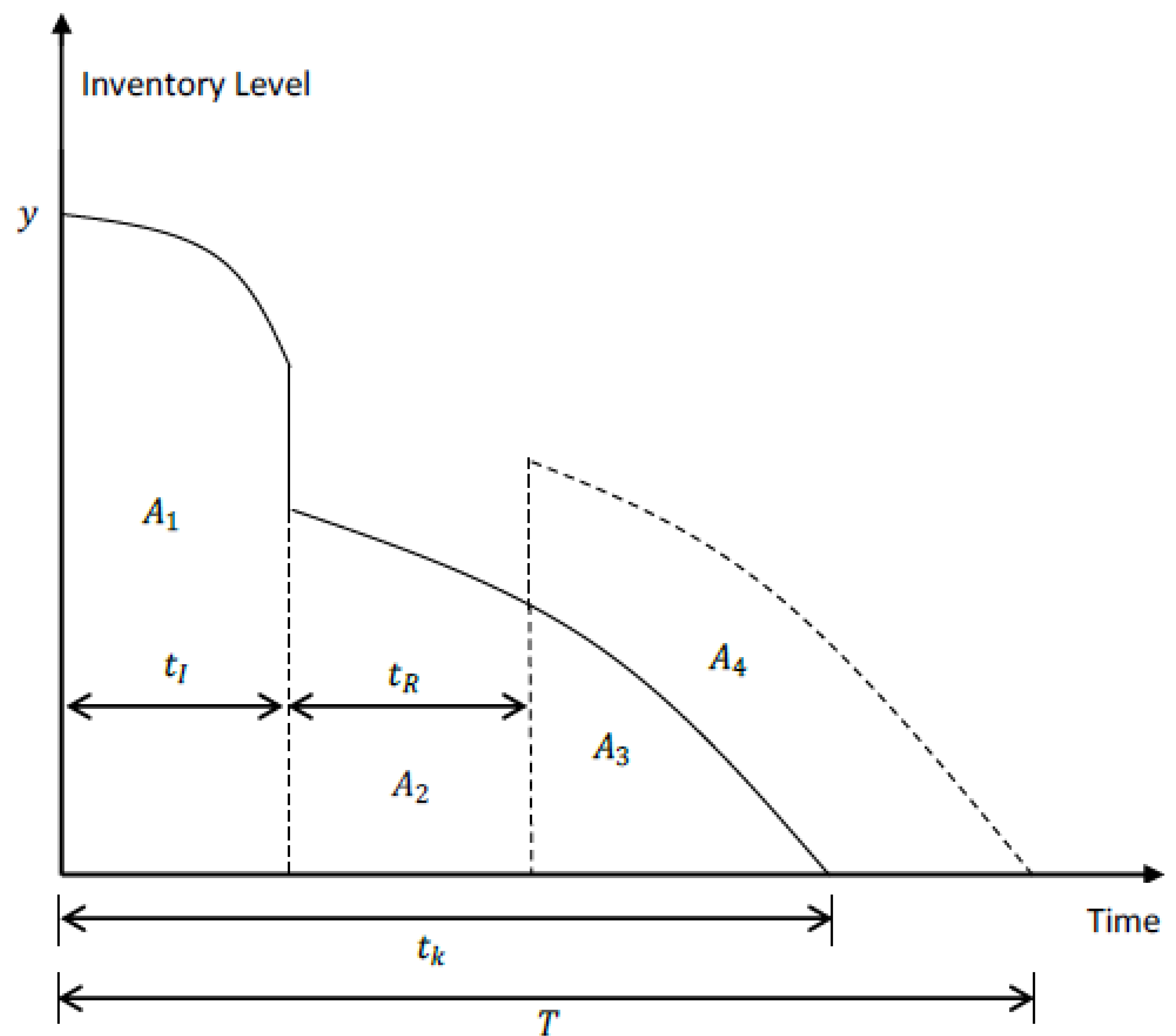
4.1. Policy 1: Repairing Defective Items

The first option treats imperfect items by sending them to be repaired at a third-party facility (Figure 1). After restoration, the items are returned to the inventory. At the beginning of each batch, a lot of y is received and depleted at the rate of D. The derivation begins by assuming a linear function for the demand rate:

$$\begin{array}{c}\hfill \frac{du}{dt}=-D=-a-bt,a,b>0\end{array}$$

(1)

The inventory function, $Y\left(t\right)$ is obtained by integration:

$$\begin{array}{ccc}\hfill {\int }_y^{Y\left(t\right)}du& =& {\int }_0^t(-a-bt)dt\hfill \\ \hfill Y\left(t\right)& =& y-at-\frac{b{t}^2}{2}.\hfill \end{array}$$

(2)

The boundary condition, $Y\left(T\right)=0$ gives

$$\begin{array}{c}\hfill y=aT+\frac{b{T}^2}{2},\end{array}$$

(3)

and from

$$\begin{array}{ccc}\hfill {\int }_{Y\left(t_I\right)-\rho y}^{0}du& =& {\int }_{t_I}^{t_k}(-a-bt)dt,\hfill \end{array}$$

we obtain

$$\begin{array}{ccc}\hfill Y\left(t_I\right)& =& \rho y+a{t}_k+\frac{b{t}_k^2}{2}-a{t}_I-\frac{b{t}_I^2}{2}.\hfill \end{array}$$

(4)

Substituting $t_I$ into (2), we obtain $Y\left(t_I\right)=y-a{t}_I-\frac{b{t}_I^2}{2}$ and substituting (3) into (4) gives

$$\begin{array}{c}\hfill y-a{t}_I-\frac{b{t}_I^2}{2}=\rho \left(aT+\frac{b{T}^2}{2}\right)+a{t}_k+\frac{b{t}_k^2}{2}-a{t}_I-\frac{b{t}_I^2}{2}.\end{array}$$

Thus,

$$\begin{array}{ccc}\hfill t_k^2& =& \frac{-2a{t}_k+(1-\rho )(2aT+b{T}^2)}{b}.\hfill \end{array}$$

(5)

Multiply Equation (5) with $t_k$ and then replace the term $t_k^2$ on the right side with (5) gives

$$\begin{array}{ccc}\hfill t_k^3& =& \frac{[b(1-\rho )(2aT+b{T}^2)+4a^2]t_k-2a(1-\rho )(2aT+b{T}^2)}{b^2}.\hfill \end{array}$$

(6)

Equations (5) and (8) will be used later for which both of the terms $t_k^2$ and $t_k^3$ can be replaced by equations in terms of $t_k$ only.

The area during the repair interval is

$$\begin{array}{ccc}\hfill A_1+A_2+A_3& =& {\int }_0^{t_I}Y\left(t\right)dt+{\int }_{t_I}^{t_k}Y\left(t\right)-\rho ydt\hfill \\ & =& {\int }_0^{t_I}y-at-\frac{b{t}^2}{2}dt+{\int }_{t_I}^{t_k}(1-\rho )y-at-\frac{b{t}^2}{2}dt\hfill \end{array}$$

(7)

$$\begin{array}{ccc}& \hspace{1em}\hspace{1em}\hspace{1em}\hspace{1em}\hspace{1em}\hspace{1em}\hspace{1em} & =((1-\rho )t_k+\rho t_I)y-\frac{a{t}_k^2}{2}-\frac{b{t}_k^3}{6}\hfill \\ & \hspace{1em}\hspace{1em}\hspace{1em}\hspace{1em}\hspace{1em}\hspace{1em}\hspace{1em} & =\frac{[2b(1-\rho )(2aT+b{T}^2)+2a^2]t_k}{6b}-\frac{a(1-\rho )(2aT+b{T}^2)}{6b}\hfill \\ & & \hspace{1em}+\frac{\rho {(2aT+b{T}^2)}^2}{4X}\hfill \end{array}$$

(8)

where the final equation is obtained from (3), (5), (6) and $t_I=\frac{y}{X}=\frac{2aT+b{T}^2}{2X}$. Next, from $t_R=\frac{\rho y}{R}+t_T=\frac{\rho (2aT+b{T}^2)}{2R}+t_T$, (3) and (7), we obtain

$$\begin{array}{ccc}\hfill A_4& =& {\int }_{t_I+t_R}^{T}Y\left(t\right)dt-{\int }_{t_I+t_R}^{t_k}Y\left(t\right)-\rho ydt\hfill \\ & =& {\int }_{t_k}^{T}y-at-\frac{b{t}^2}{2}dt-{\int }_{t_I+t_R}^{t_k}\rho ydt\hfill \\ & =& y(T-t_k)-\frac{a{T}^2}{2}-\frac{b{T}^3}{6}+\frac{a{t}_k^2}{2}+\frac{b{t}_k^3}{6}+\rho y(t_k-t_I-t_R)\hfill \\ & =& -\left(((1-\rho )t_k+\rho t_I)y-\frac{a{t}_k^2}{2}-\frac{b{t}_k^3}{6}\right)-\rho y{t}_R+yT-\frac{a{T}^2}{2}-\frac{b{T}^3}{6}\hfill \\ & =& -(A_1+A_2+A_3)-\frac{\rho t_T(2aT+b{T}^2)}{2}-\frac{{\rho }^2{(2aT+b{T}^2)}^2}{4R}+\frac{a{T}^2}{2}+\frac{b{T}^3}{3}.\hfill \end{array}$$

(9)

Since $\rho y$ units need to be sent for repair, the total payment for repair is $c_1\rho y$. In addition, the amount that needs to be paid for transportation is $2c_T\rho y$. In particular, the transportation cost considers the two-way transport, that is, the cost for delivering the imperfect items to the repair facility and the cost for resending the repaired items from the repair facility. The holding cost at the repair facility is denoted by $h^{\prime }{t}_R\rho y$. Note that a fixed amount of repair setup cost and transportation fixed cost needs to be paid. The markup percentage by the repair shop is included in the calculation of the total cost of each repaired item, $c_R\left(y\right)$. Hence, the following equation is obtained:

$$\begin{array}{ccc}\hfill c_R\left(y\right)& =& (1+m)\left(\frac{S+2A}{\rho y}+c_1+2c_T+h^{\prime }{t}_R\right).\hfill \end{array}$$

The holding cost per cycle, $HC\left(y\right)$ is determined by calculating the area under the curve. Therefore,

$$\begin{array}{ccc}\hfill HC\left(y\right)& =& h(A_1+A_2+A_3)+h_R{A}_4.\hfill \end{array}$$

The total cost per unit, $TC\left(y\right)$ is given by

$$\begin{array}{ccc}\hfill TC\left(y\right)& =& K+(c_u+c_I)y+c_R\left(y\right)\rho y+HC\left(y\right).\hfill \end{array}$$

The objective function, which is the total profit per unit time, $TPU\left(y\right)$, is equal to the total revenue per cycle minus the total cost per cycle divided by the cycle time, that is

$$\begin{array}{ccc}\hfill TPU\left(y\right)& =& \frac{Py-TC\left(y\right)}{T}.\hfill \end{array}$$

After the value of $T^{*}$ that maximises $TPU$ is obtained, the optimal order size, $y^{*}$, can be calculated. We choose the variable T for calculations so that the process becomes less tedious. Furthermore, this can be achieved as y can be expressed as a function of T (see (3)). Now,

$$\begin{array}{ccc}\hfill \frac{TC\left(T\right)}{T}& =& \frac{1}{T}[K+(c_u+c_I)y+c_R\left(y\right)\rho y+HC\left(T\right)]\hfill \\ & =& \frac{K}{T}+(c_u+c_I)\left[\frac{2a+bT}{2}\right]+(1+m)\left\{\left[\frac{S+2A}{T}\right]+(c_1+2c_T)\rho \left[\frac{2a+bT}{2}\right]\right\}\hfill \\ & & +h^{{}^{\prime }}(1+m)\left\{\frac{{\rho }^2(2aT+b{T}^2)(2a+bT)}{4R}+t_T\rho \left[\frac{2a+bT}{2}\right]\right\}+\frac{HC\left(T\right)}{T}.\hfill \end{array}$$

(10)

By Equations (8) and (9),

$$\begin{array}{ccc}\hfill \frac{HC\left(T\right)}{T}& =& \frac{1}{T}[(h-h_R)(A_1+A_2+A_3)+\hfill \\ & & +h_R\left(\frac{a{T}^2}{2}+\frac{b{T}^3}{3}-\frac{\rho t_T(2aT+b{T}^2)}{2}-\frac{{\rho }^2{(2aT+b{T}^2)}^2}{4R}\right)]\hfill \\ & =& (h-h_R)\left(\frac{2b(1-\rho )(2a+bT)t_k}{6b}+\frac{a^2{t}_k}{3bT}-\frac{a(1-\rho )(2a+bT)}{6b}+\frac{\rho (2aT+b{T}^2)(2a+bT)}{4X}\right)+\hfill \\ & & +h_R\left(\frac{aT}{2}+\frac{b{T}^2}{3}-\frac{\rho t_T(2a+bT)}{2}-\frac{{\rho }^2(2aT+b{T}^2)(2a+bT)}{4R}\right).\hfill \end{array}$$

(11)

Using Equations (10) and (11), we obtain

$$\begin{array}{ccc}\hfill TPU\left(T\right)& =& \frac{Py-TC\left(T\right)}{T}\hfill \\ & =& \left[\frac{2a+bT}{2}\right]Z_1+\left[\frac{(2aT+b{T}^2)(2a+bT)}{4}\right]Z_2\hfill \\ & & +\left[\frac{aT}{2}+\frac{b{T}^2}{3}\right]Z_3+\frac{Z_4}{T}+(2a+bT)t_k{Z}_5+\frac{t_k}{T}{Z}_6.\hfill \end{array}$$

(12)

where the constants $Z_1,Z_2,Z_3,Z_4,Z_5$ and $Z_6$ are defined as follows:

$$\begin{array}{ccc}\hfill Z_1& =& P-c_u-c_I-(1+m)(c_1+2c_T+h^{{}^{\prime }}{t}_T)\rho +h_R\rho t_T+\frac{a(1-\rho )(h-h_R)}{3b};\hfill \\ \hfill Z_2& =& \frac{h_R{\rho }^2}{R}-\frac{\rho (h-h_R)}{X}-\frac{h^{{}^{\prime }}{\rho }^2(1+m)}{R};\hfill \\ \hfill Z_3& =& -h_R;\hfill \\ \hfill Z_4& =& -[K+(1+m\left)\right(S+2A\left)\right];\hfill \\ \hfill Z_5& =& -(h-h_R)\left[\frac{2b(1-\rho )}{6b}\right];\hfill \\ \hfill Z_6& =& -(h-h_R)\left(\frac{a^2}{3b}\right).\hfill \end{array}$$

Equation (5) is quadratic, so, yielding

$$\begin{array}{ccc}\hfill t_k& =& \sqrt{{\left(\frac{a}{b}\right)}^2+(1-\rho )\left[2\left(\frac{a}{b}\right)T+T^2\right]}-\frac{a}{b}.\hfill \end{array}$$

Next, we find the first and second derivatives of $t_k$ with respect to T.

$$\begin{array}{c}\hfill \frac{d{t}_k}{dT}=\frac{(1-\rho )\left[\left(\frac{a}{b}\right)+T\right]}{\sqrt{{\left(\frac{a}{b}\right)}^2+(1-\rho )\left[2\left(\frac{a}{b}\right)T+T^2\right]}}.\end{array}$$

(13)

$$\begin{array}{c}\hfill \frac{d^2{t}_k}{d{T}^2}=\frac{(1-\rho )}{\sqrt{{\left(\frac{a}{b}\right)}^2+(1-\rho )\left[2\left(\frac{a}{b}\right)T+T^2\right]}}-\frac{{(1-\rho )}^2{\left(\frac{a}{b}+T\right)}^2}{{\left\{{\left(\frac{a}{b}\right)}^2+(1-\rho )\left[2\left(\frac{a}{b}\right)T+T^2\right]\right\}}^{\frac{3}{2}}}.\end{array}$$

(14)

Calculating the derivatives of $t_k$ allows $TPU\left(T\right)$ to be differentiated with respect T:

$$\begin{array}{ccc}\hfill \frac{dTPU\left(T\right)}{dT}& =& \left(\frac{b}{2}\right)Z_1+\left[\frac{(2a+3bT)(2a+bT)}{4}\right]Z_2+\left(\frac{a}{2}+\frac{2bT}{3}\right)Z_3-\frac{Z_4}{T^2}\hfill \\ & & +\left[b{t}_k+(2a+bT)\frac{d{t}_k}{dT}\right]Z_5+\left(\frac{1}{T}\frac{d{t}_k}{dT}-\frac{t_k}{T^2}\right)Z_6.\hfill \end{array}$$

(15)

The necessary condition for $TPU\left(T\right)$ to be a maximum is

$$\frac{dTPU\left(T\right)}{dT}=0.$$

Hence, the value of $T^{*}$ is obtained by setting $\frac{dTPU\left(T\right)}{dT}$ to be zero and solving the equation for $T^{*}$. Then, the optimal stock quantity is calculated by the following formula:

$$y^{*}=a{T}^{*}+\frac{b{\left(T^{*}\right)}^2}{2}$$

To verify that the obtained value $T^{*}$ indeed maximizes $TPU$, the second derivative of $TPU\left(T\right)$ is computed:

$$\begin{array}{ccc}\hfill \frac{d^{2}TPU\left(T\right)}{dT}& =& \left[\frac{8ba+6b^{2}T}{4}\right]Z_2+\left(\frac{2b}{3}\right)Z_3+\frac{2}{T^3}{Z}_4\hfill \\ & & +\left[2b\frac{d{t}_k}{dT}+(2a+bT)\frac{d^2{t}_k}{d{T}^2}\right]Z_5\hfill \\ & & +\left(-\frac{2}{T^2}\frac{d{t}_k}{dT}+\frac{1}{T}\frac{d^2{t}_k}{d{T}^2}+\frac{2t_k}{T^3}\right)Z_6.\hfill \end{array}$$

(16)

The value of $\frac{d^{2}TPU\left(T\right)}{dT}$ obtained at $T=T^{*}$ must be negative. This is an indication that $TPU\left(T^{*}\right)$ is maximum.

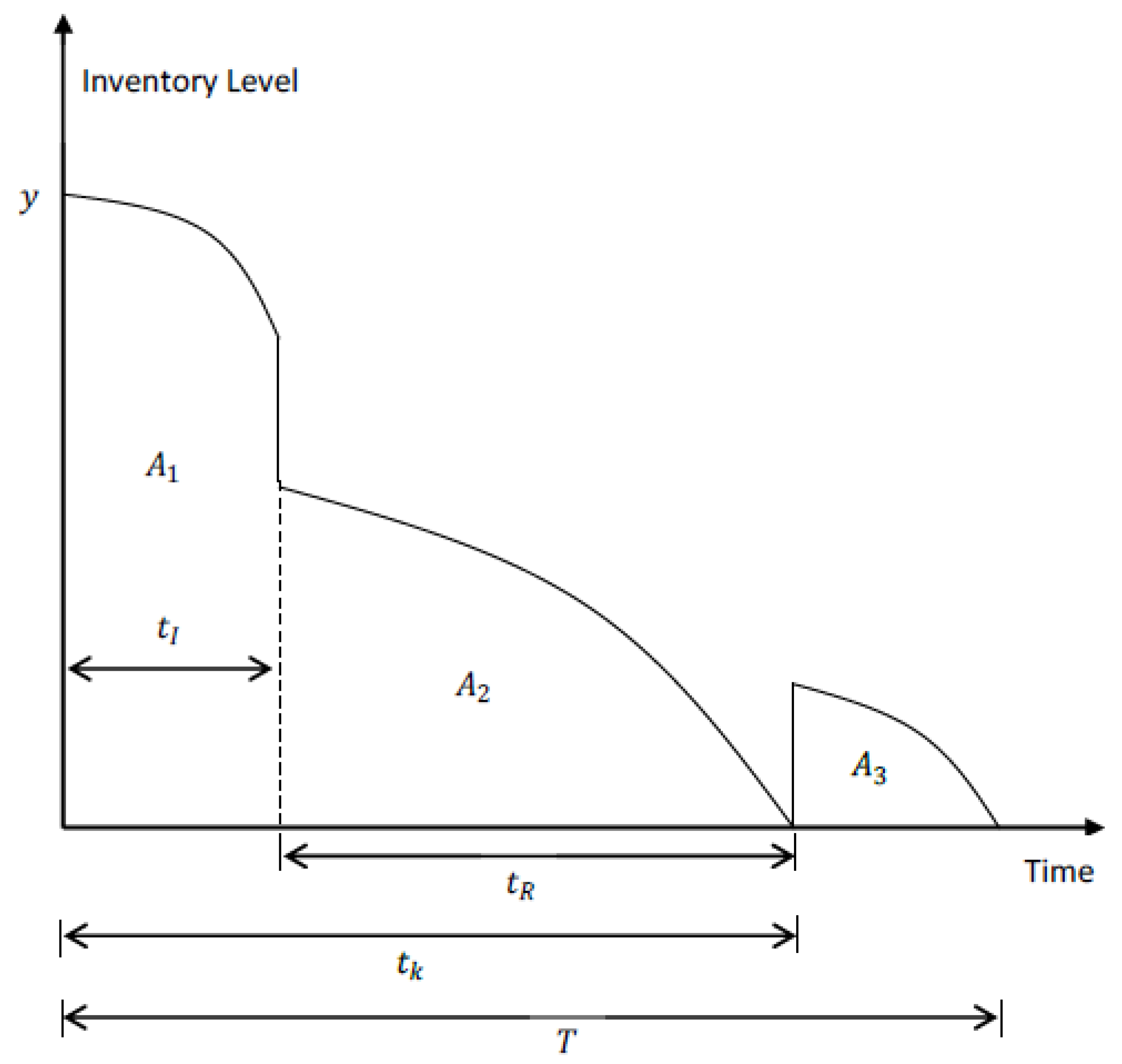
4.2. Policy 2: Buying New Items to Replace Defective Items

In the second option, faulty items are replaced by purchasing the same number of items from an alternate local supplier but at an increased price (Figure 2).

Repeating the same process as in the first model considered, it can be observed that Equations (3) and (5) still hold.

As in Equation (8), it can be shown that

$$\begin{array}{ccc}\hfill A_1+A_2& =& {\int }_0^{t_I}Y\left(t\right)dt+{\int }_{t_I}^{t_k}Y\left(t\right)-\rho ydt\hfill \\ & =& \frac{[2b(1-\rho )(2aT+b{T}^2)+2a^2]t_k}{6b}-\frac{a(1-\rho )(2aT+b{T}^2)}{6b}\hfill \\ & & +\frac{\rho {(2aT+b{T}^2)}^2}{4X}\hfill \end{array}$$

(17)

By Equation (1), the expression for $Y\left(t\right)$ for $t_k\le t\le T$ can be obtained by integrating the following expression

$$\begin{array}{ccc}\hfill {\int }_{\rho y}^{Y\left(t\right)}du& =& {\int }_{t_k}^T-a-btdt.\hfill \end{array}$$

(18)

Hence,

$$\begin{array}{ccc}\hfill Y\left(t\right)& =& \rho y-at-\frac{b{t}^2}{2}+a{t}_k+\frac{b{t}_k^2}{2}.\hfill \end{array}$$

(19)

Using this expression, we obtain

$$\begin{array}{ccc}\hfill A_3& =& {\int }_{t_k}^{T}Y\left(t\right)dt\hfill \\ & =& {\int }_{t_k}^T\rho y-at-\frac{b{t}^2}{2}+a{t}_k+\frac{b{t}_k^2}{2}dt\hfill \\ & =& \rho y(T-t_k)-\frac{a{T}^2}{2}-\frac{b{T}^3}{6}+\frac{a{t}_k^2}{2}+\frac{b{t}_k^3}{6}+\left(a{t}_k+\frac{b{t}_k^2}{2}\right)(T-t_k).\hfill \end{array}$$

(20)

Adding Equations (17) and (20) together, and then replace the term $t_k^2$ with the expression in (5), we obtain

$$\begin{array}{ccc}\hfill A_1+A_2+A_3& =& \left[y(1-2\rho )-\frac{(1-\rho )(2aT+b{T}^2)}{2}\right]t_k+\rho y\left(T+\frac{2aT+b{T}^2}{2X}\right)-\frac{a{T}^2}{2}-\frac{b{T}^3}{6}\hfill \\ & & +\left[\frac{(1-\rho )(2a{T}^2+b{T}^3)}{2}\right],\hfill \end{array}$$

which implies that

$$\begin{array}{ccc}\hfill A_3& =& -(A_1+A_2)+\left[y(1-2\rho )-\frac{(1-\rho )(2aT+b{T}^2)}{2}\right]t_k+\rho y\left(T+\frac{2aT+b{T}^2}{2X}\right)\hfill \\ & & -\frac{a{T}^2}{2}-\frac{b{T}^3}{6}+\left[\frac{(1-\rho )(2a{T}^2+b{T}^3)}{2}\right].\hfill \end{array}$$

(21)

The holding cost is given by

$$HC\left(y\right)=h(A_1+A_2)+h_E{A}_3.$$

The total cost per unit, $TC\left(y\right)$ is given by

$$\begin{array}{ccc}\hfill TC\left(y\right)& =& K+(c_u+c_l+\rho (c_E-c_s))y+HC\left(T\right).\hfill \end{array}$$

The objective function, which is the total profit per unit time, $TPU\left(y\right)$, is equal to the total revenue per cycle minus the total cost per cycle divided by the cycle time, that is

$$\begin{array}{ccc}\hfill TPU\left(y\right)& =& \frac{Py-TC\left(y\right)}{T}.\hfill \end{array}$$

After the value of $T^{*}$, which maximises $TPU$, is obtained, the optimal order size, $y^{*}$, can be calculated. As in Policy 1, we choose the variable T for calculations to make the process less tedious.

Now, the total cost per unit for one cycle is

$$\begin{array}{ccc}\hfill \frac{TC\left(T\right)}{T}& =& \frac{K}{T}+[c_u+c_I+\rho (c_E-c_s)]\left(\frac{2a+bT}{2}\right)+\frac{HC\left(T\right)}{T}\hfill \end{array}$$

(22)

By Equations (17) and (21),

$$\begin{array}{ccc}\hfill \frac{HC\left(T\right)}{T}& =& \frac{1}{T}[(h-h_E)(A_1+A_2)+\hfill \\ & & +h_E(\left(y(1-2\rho )-\frac{(1-\rho )(2aT+b{T}^2)}{2}\right)t_k+\rho y\left(T+\frac{2aT+b{T}^2}{2X}\right)\hfill \\ & & -\frac{a{T}^2}{2}-\frac{b{T}^3}{6}+\frac{(1-\rho )(2a{T}^2+b{T}^3)}{2}\left)\right]\hfill \\ & =& h\left(\frac{(1-\rho )(2a+bT)t_k}{3}+\frac{a^2{t}_k}{3bT}-\frac{a(1-\rho )(2a+bT)}{6b}+\frac{\rho (2a+bT)(2aT+b{T}^2)}{4X}\right)\hfill \\ & & +h_E\left(\frac{aT}{2}+\frac{b{T}^2}{3}-\frac{(2+\rho )(2a+bT)t_k}{6}-\frac{a^2{t}_k}{3bT}+\frac{a(1-\rho )(2a+bT)}{6b}\right).\hfill \end{array}$$

(23)

Using Equations (22) and (23), the total unit time profit is

$$\begin{array}{ccc}\hfill TPU\left(T\right)& =& \frac{Py-TC\left(T\right)}{T}\hfill \\ & =& \left[\frac{2a+bT}{2}\right]Z_1+\left[\frac{(2aT+b{T}^2)(2a+bT)}{4}\right]Z_2\hfill \\ & & +\left[\frac{aT}{2}+\frac{b{T}^2}{3}\right]Z_3+\frac{Z_4}{T}+(2a+bT)t_k{Z}_5+\frac{t_k}{T}{Z}_6.\hfill \end{array}$$

(24)

where the constants $Z_1,Z_2,Z_3,Z_4,Z_5$ and $Z_6$ are defined as follows:

$$\begin{array}{ccc}\hfill Z_1& =& P-[c_u+c_I+\rho (c_E-c_s)]+(h-h_E)\frac{a(1-\rho )}{3b};\hfill \\ \hfill Z_2& =& -\frac{h\rho }{X};\hfill \\ \hfill Z_3& =& -h_E;\hfill \\ \hfill Z_4& =& -K;\hfill \\ \hfill Z_5& =& -\frac{2h(1-\rho )-h_E(2+\rho )}{6};\hfill \\ \hfill Z_6& =& -(h-h_E)\frac{a^2}{3b}.\hfill \end{array}$$

As in Policy 1, we find the value of $T^{*}$ that maximises $TPU$.

5. Numerical Example and Sensitivity Analysis

A numerical analysis is carried out to compare the two mathematical models presented in Section 4. By performing a numerical analysis of the two models using the same parameters, the model that provides the optimal policy can be discovered. This approach is useful as the parameters can be easily modified to fit real-life situations. In this section, the input parameters of the numerical examples from Jaber et al. [2] are adopted. Recall that the demand rate considered by them is constant. The reason for choosing the same parameters as theirs is that a comparison can be made under the assumption of a linear demand rate for different values of b. The input parameters are as follows:

K = $100, A = $200, S = $100, P = $50/unit, $c_I$ = $0.5/unit, $c_u$ = $25/unit, $c_s$ = $20/unit,

$c_T$ = $2/unit, $c_1$ = $5/unit, $c_E$ = $40/unit, h = $5/unit/year, $h^{{}^{\prime }}$ = $4/unit/year,

$h_R$ = $6/unit/year, $h_E$ = $8/unit/year, X = 175,200 units/year, D = 50,000 units/year,

R = 50,000 units/year, $t_T$ = 2/200 year, m = 20%, and $\rho$ = 0.02.

The solution to the equation $TP{U}^{{}^{\prime }}\left(T\right)=0$ for both policies is solved using Wolfram Mathematica. Fixing the parameters as stated above, the solution to the equation, $T^{*}$ which satisfies $0<T^{*}<1$, is used to decide the optimal model. Since the demand function is linear, the following outputs (

Table 2. Solutions for both policies.

Policy 1	Policy 2
$T^{*}=0.075$	$T^{*}=0.029$
$TPU\left(T^{*}\right)=1,195,456.243$	$TPU\left(T^{*}\right)=1,198,028.718$
$TP{U}^{{}^{\prime }}\left(T^{*}\right)$ ≈ 0	$TP{U}^{{}^{\prime }}\left(T^{*}\right)$ ≈ 0
$TP{U}^{{}^{″}}\left(T^{*}\right)=-365,714.468$	$TP{U}^{{}^{″}}\left(T^{*}\right)=-8,469,934.328$
$y^{*}=3732.409$	$y^{*}=1434.457$

) are computed for the case a = 50,000 and $b=5$.

Figure 3 shows the total unit time profit, $TPU$, for both policies. It can be seen that although Policy 2 generates a higher maximum total profit per unit time than that of Policy 1 at the beginning, the value of $TPU$ for Policy 2 decreases rapidly after the value of T exceeds $T^{*}$. As T differs from 0 to 1, it is obvious that the graph of Policy 1 is above Policy 2 more frequently, implying that Policy 1 generates a higher total profit per unit time more consistently than Policy 2. To put it differently, the rate of decrease in $TPU$ in Policy 1 is lower than the rate of decrease in $TPU$ in Policy 2 after the inventory level exceeds the optimal stock quantity, resulting in Policy 1 being chosen as the most suitable model. From Equation (3), note that the amount of stock, y, increases as the total duration of the model, T, increases. In other words, the greater the T is, the greater the y is. If there is no restriction on the order quantity, then Policy 2 outperforms Policy 1. However, in real life, a vendor may require a buyer to order a minimum amount of items. For this scenario, Policy 1 outperforms Policy 2, as shown by the mathematical models of the two policies.

Table 3. The solutions for both policies with varying values of b.

	Policy 1					Policy 2
b	$T^{*}$	$y^{*}$	$t_l$	$t_R$	$t_k$	$T^{*}$	$y^{*}$	$t_l$	$t_R$	$t_k$
5000	0.1025	5149.1465	0.0294	0.0112	0.1004	0.0402	2012.6031	0.0115	0.0279	0.0394
500	0.0765	3824.4618	0.0218	0.0106	0.0749	0.0294	1470.9296	0.0084	0.0204	0.0288
50	0.0748	3740.5108	0.0213	0.0106	0.0733	0.0288	1437.6622	0.0082	0.0200	0.0282
5	0.0746	3732.4093	0.0213	0.0106	0.0732	0.0287	1434.4571	0.0082	0.0199	0.0281
0.5	0.0746	3731.6020	0.0213	0.0106	0.0731	0.0287	1434.1377	0.0082	0.0199	0.0281
0.05	0.0746	3731.5213	0.0213	0.0106	0.0731	0.0287	1434.1058	0.0082	0.0199	0.0281

shows the behaviour of Policies 1 and 2 while varying the value of b when $a=\mathrm{50,000}$. As shown in Jaber et al. [2], the optimal amount of stock is $y^{*}=3732$ for Model 1 and $y^{*}=1434$ for Model 2 when the demand function is constant. From the sensitivity analysis, the values of $y^{*}$ and $TPU\left(T^{*}\right)$ for both models tend to reach their optimal values in the constant case as b approaches 0. Therefore, the results obtained here can be considered as generalisations of the results obtained by Jaber et al. [2].

6. Theoretical and Managerial Implications

This study offers several managerial insights to companies for effectively managing or coping with intricacy and becoming more inventive. Based on the analysis results performed in Section 5, we have identified the following managerial implications, which will be beneficial to a company’s management team:

(1)

The buyer should not perceive the imperfect items as second-grade products and unreservedly sell them at a discounted price. In point of fact, there are other better options available, such as

(i)

Send those imperfect items to a local workshop for repair and sell them at full price once they have been fixed;

(ii)

Purchase new items from a local supplier as replacements for those imperfect items and trade them at full price.

(2)

If the purchased quantity is small, a buyer should opt for Policy 2, i.e., replace the imperfect items with those new purchased from a local supplier. This suggestion is valid because the total profit per unit under Policy 2 achieves the highest at the beginning of the total time cycle (see Figure 3). To explain more practically, a small number of stock orders implies a small number of imperfect items; it is not worth sending the imperfect items for repair as this approach takes longer to return to capital.

(3)

If a large quantity purchase is required, a buyer should undoubtedly opt for Policy 1, i.e., send the imperfect items to a local workshop for repair purposes. This advice works because the graph of the total profit per unit for Policy 1 is predominantly above that for Policy 2 (see Figure 3). That is to say, from the long-term perspective, repairing the imperfect items from large stocks will bring the company a consistent profit.

We note here that the implications (1)–(3) hold during the growth and maturity stages of the product cycle.

7. Conclusions

Two modified EOQ models are presented in this paper where the first model deals with Policy 1 and the second model deals with Policy 2. The outcome obtained here offers beneficial insights and provides salvaging options for a firm to handle imperfect quality items. Policy 1 suggests that imperfect quality items are sent for repairs, whereas Policy 2 suggests that imperfect quality items are replaced by purchasing new items from a local supplier at a higher price. The work of Jaber et al. [2] is extended in this research in the sense that the demand function considered here is linearly increasing. Our emphasis here is that Jaber et al. considered the above two policies under the assumption of a constant demand rate, which is only valid during the maturity phase of a product life cycle. In response to different phases of a product life cycle, different corresponding demand rates are worth exploring. What is the best policy to tackle the problem of defective products in the growth stage of a product life cycle? This is the core of our research, and in this paper, the growth stage of a product life cycle is considered, and the demand rate is assumed to be linearly increasing. It should be noted here that the sensitivity analysis in Table 3 shows that the value of the optimal amount of stock $y^{*}$ approaches the value of the optimal stock quantity obtained by Jaber et al. [2] when the linear demand function approaches the constant demand function. Therefore, our developed mathematical models are indeed generalisations of the models obtained by Jaber et al. [2].

Our findings reveal that Policy 2 performs better than Policy 1 if there is no restriction on the number of ordered stock items for a buyer. This situation is not always accurate in real life, as a vendor may set a threshold on the minimum purchased items to stimulate sales. As a result, Policy 1 may be superior to Policy 2 in this scenario. We note here that the results in this research support the findings obtained by Jaber et al. [2]. They also drew similar conclusions as ours. Therefore, it can be concluded that either in the growth stage or the maturity stage of a product life cycle, the choice of Policy 1 or 2 depends on whether there is any restriction on the minimum amount of items that need to be ordered by a buyer. Generally speaking, if the ordered quantity is small, then the best option is to replace the imperfect items by purchasing new items from a local supplier at a higher price. On the contrary, if the ordered quantity is large, then the best option is to send the imperfect items for repairs to a third-party facility.

The work performed in this research can be extended in a myriad of ways. Firstly, future researchers may consider other options to handle imperfect quality items, such as obtaining machinery and manpower to fix defective items in the firm instead of sending defective items to a shop for repairs. By considering this alternative, transportation and repair costs can be cut down but at the cost of increased machinery and labour costs. Another option to handle imperfect quality items is to return the defective items to the original supplier to be recycled, and an equal number of items are repurchased to replace the defective items. If this option is considered, the firm will have to handle an increased cost of transportation, but the cost of the items during the second purchase may be decreased since the materials used to produce the items are provided by the firm.

The case where the demand function is quadratic or of a higher degree can also be considered in future work. Will the result obtained still be consistent with the work of Jaber et al. [2] when the demand function is now quadratic or cubic? This will be an exhilarating mathematical exercise for interested readers in the future.

References

1. Khanra, S.; Chaudhuri, K.S. A note on an order-level inventory model for a deteriorating item with time-dependent quadratic demand. Comput. Oper. Res. 2003, 30, 1901–1916. [Google Scholar] [CrossRef]
2. Jaber, M.Y.; Zanoni, S.; Zavanella, L.E. Economic order quantity models for imperfect items with buy and repair options. Int. J. Prod. Econ. 2014, 155, 126–131. [Google Scholar] [CrossRef]
3. Yoo, S.H.; Kim, D.; Park, M.S. Economic production quantity model with imperfectquality items, two-way imperfect inspection and sales return. Int. J. Prod. Econ. 2009, 121, 255–265. [Google Scholar] [CrossRef]
4. Khan, M.; Jaber, M.Y.; Bonney, M. An economic order quantity (EOQ) for items with imperfect quality and inspection errors. Int. J. Prod. Econ. 2011, 133, 113–118. [Google Scholar] [CrossRef]
5. Khan, M.; Jaber, M.Y.; Guiffrida, A.L.; Zolfaghari, S. A review of the extensions of a modified EOQ model for imperfect quality items. Int. J. Prod. Econ. 2011, 132, 1–12. [Google Scholar] [CrossRef]
6. Dey, O.; Giri, B.C. A new approach to deal with learning in inspection in an integrated vendor-buyer model with imperfect production process. Comput. Ind. Eng. 2019, 131, 515–523. [Google Scholar] [CrossRef]
7. Hsu, J.T.; Hsu, L.F. An EOQ model with imperfect quality items, inspection errors, shortage backordering, and sales returns. Int. J. Ind. Eng. Comput. 2013, 143, 162–170. [Google Scholar] [CrossRef]
8. Khalilpourazari, S.; Pasandideh, S.H.R.; Niaki, S.T.A. Optimizing a multi-item economic order quantity problem with imperfect items, inspection errors, and backorders. Soft Comput. 2019, 23, 11671–11698. [Google Scholar] [CrossRef]
9. Al-Salamah, M. Economic production quantity in batch manufacturing with imperfect quality, imperfect inspection, and destructive and non-destructive acceptance sampling in a two-tier market. Comput. Ind. Eng. 2016, 93, 275–285. [Google Scholar] [CrossRef]
10. Al-Salamah, M. Economic production quantity in an imperfect manufacturing process with synchronous and asynchronous flexibility rework rates. Oper. Res. Perspect. 2019, 6, 100103. [Google Scholar]
11. Bose, D.; Guha, A. Economic production lot sizing under imperfect quality, on-line inspection, and inspection errors: Full vs. sampling inspection. Comput. Ind. Eng. 2021, 160, 107565. [Google Scholar] [CrossRef]
12. Cheikhrouhou, N.; Sarkar, B.; Ganguly, B.; Malik, A.I.; Batista, R.; Lee, Y.H. Optimization of sample size and order size in an inventory model with quality inspection and return of defective items. Ann. Oper. Res. 2018, 271, 445–467. [Google Scholar] [CrossRef] [Green Version]
13. Chen, C.H.; Tsai, C.H. The modified economic manufacturing quantity model based on inspection error, quality loss, and shortage. J. Inf. Optim. Sci. 2015, 36, 511–531. [Google Scholar] [CrossRef]
14. Genta, G.; Galetto, M.; Franceschini, F. Inspection procedures in manufacturing processes: Recent studies and research perspectives. Int. J. Prod. Res. 2020, 58, 4767–4788. [Google Scholar] [CrossRef]
15. Ouyang, L.Y.; Su, C.H.; Ho, C.H.; Yang, C.T. Optimal ordering policy for an economic order quantity model with inspection errors and inspection improvement investment. Int. J. Inf. Manag. Sci. 2014, 25, 317–330. [Google Scholar]
16. Salameh, M.K.; Jaber, M.Y. Economic production quantity model for items with imperfect quality. Int. J. Prod. Econ. 2000, 64, 59–64. [Google Scholar] [CrossRef]
17. Dye, C.Y.; Hsieh, T.P. A Particle Swarm Optimization for Solving Lot-Sizing Problem with Fluctuating Demand and Preservation Technology Cost under Trade Credit. J. Glob. Optim. 2013, 55, 655–679. [Google Scholar] [CrossRef]
18. Idris, A.N. Opportunities in a Crisis. The Edge Financial Daily. 2020. Available online: https://www.theedgemarkets.com/article/opportunities-crisis (accessed on 10 April 2022).
19. Goyal, S.K.; Giri, B. Recent trends in modeling of deteriorating inventory. Eur. J. Oper. Res. 2001, 134, 1–16. [Google Scholar] [CrossRef]
20. Hariga, M.; Alyan, A.A. A lot sizing heuristic for deteriorating items with shortages in growing and declining markets. Comput. Oper. Res. 1997, 24, 1075–1083. [Google Scholar] [CrossRef]
21. Musa, S.; Supadi, S.S.; Omar, M. The optimal manufacturing batch size with rework under time-varying demand process for a finite time horizon. AIP Conf. Proc. 2015, 1605, 1105–1110. [Google Scholar]
22. Chang, H.J.; Hung, C.H.; Dye, C.Y. A finite time horizon inventory model with deterioration and timevalue of money under the conditions of permissible delay in payments. Int. J. Syst. Sci. 2002, 33, 141–151. [Google Scholar] [CrossRef]
23. Xu, C.; Liu, X.; Wu, C.; Yuan, B. Optimal Inventory Control Strategies For Deteriorating Items With A General Time-Varying Demand Under Carbon Emission Regulations. Energies 2020, 13, 999. [Google Scholar] [CrossRef] [Green Version]
24. Usman, T.; Dari, S.; Stephen, K.; Magaji, A.S.; Nasiru, A. An economic order quantity (EOQ) model for items with linear demand, imperfect quality and inspection errors. Kasu J. Math. Sci. 2020, 1, 32–51. [Google Scholar]
25. Chen, C.K.; Hung, T.W.; Weng, T.C. A net present value approach in developing optimal replenishment policies for a product life cycle. Appl. Math. Comput. 2007, 184, 360–373. [Google Scholar] [CrossRef]
26. Chen, C.K.; Hung, T.W.; Weng, T.C. Optimal replenishment policies with allowable shortages for a product life cycle. Comput. Math. Appl. 2007, 53, 1582–1594. [Google Scholar] [CrossRef] [Green Version]
27. Cárdenas-Barrón, L.E.; Plaza-Makowsky, M.J.L.; Sevilla-Roca, M.A.; Núñez-Baumert, J.M.; Mandal, B. An inventory model for imperfect quality products with rework, distinct holding costs, and nonlinear demand dependent on price. Mathematics 2021, 9, 1362. [Google Scholar] [CrossRef]
28. Lin, T.Y. An economic order quantity with imperfect quality and quantity discounts. Appl. Math. Model. 2010, 34, 3158–3165. [Google Scholar] [CrossRef]
29. Konstantaras, I.; Skouri, K.; Jaber, M.Y. Inventory models for imperfect quality items with shortages and learning in inspection. Appl. Math. Model. 2012, 36, 5334–5343. [Google Scholar] [CrossRef]
30. Jaggi, C.K.; Goel, S.K.; Mittal, M. Credit financing in economic ordering policies for defective items with allowable shortages. Appl. Math. Comput. 2013, 219, 5268–5282. [Google Scholar] [CrossRef]
31. Sharifi, E.; Sobhanallahi, M.A.; Mirzazadeh, A.; Shabani, S. An EOQ model for imperfect quality items with partial backordering under screening errors. Cogent Eng. 2015, 2, 994258. [Google Scholar] [CrossRef]
32. Lu, Y.; Mo, J.; Wei, Y. Optimal buyer’s replenishment policy in the integrated inventory model for imperfect items. Math. Probl. Eng. 2016, 2016, 5382329. [Google Scholar]
33. Taleizadeh, A.A.; Khanbaglo, M.P.S.; Cárdenas-Barrón, L.E. An EOQ inventory model with partial backordering and reparation of imperfect product. Int. J. Prod. Econ. 2016, 182, 418–434. [Google Scholar] [CrossRef]
34. Mokhtari, H.; Asadkhani, J. Economic order quantity for imperfect quality items under inspection errors, batch replacement, and multiple sales of returned items. Sci. Iran. 2021, 28, 2890–2909. [Google Scholar] [CrossRef] [Green Version]
35. Pimsap, P.; Srisodaphol, W. Economic order quantity model of imperfect items using single sampling plan for attributes. J. Appl. Sci. Eng. 2022, 25, 1065–1073. [Google Scholar]
Figure 1. Inventory level for the repair option for the defective items (Policy 1).
Processes 10 01220 g001
Figure 2. Inventory level for the buying option to replace the defective items (Policy 2).
Processes 10 01220 g002
Figure 3. Total profit per unit (TPU) for the two different policies.
Processes 10 01220 g003