Abstract
Two-part epoxy adhesives are widely used in a range of industries. Two-part epoxy adhesive is composed of a resin and a hardener. Both materials remain stable in the general environment but curing begins when mixed in the specified mixing ratio. However, it has the disadvantage of requiring a specific mixing device. In addition, if the mixing ratio is different from the specified ratio due to the error of the mixing system, it has a fatal effect on the adhesion performance. The dielectric constant is a characteristic constant of a material. Therefore, it represents the mixing ratio of mixed two-part epoxy adhesives. With the electrical impedance spectroscopy technique, it can be measured indirectly by measuring impedance according to frequency and temperature. In this study, a sensor and embedded device for an online monitoring of its integrity using a regression method among machine learning are developed, which can acquire impedance data with frequency and temperature data according to the change in the mixing ratio of a two-part epoxy adhesive. The experimentally collected data were used as training data for the machine learning algorithm. It was found that the learned machine learning algorithm effectively estimates the mixing ratio of the two-part epoxy with an arbitrary value.
1. Two-Part Epoxy Adhesive Overview
1.1. The Importance of the Mixing Ratio of Two-Part Epoxy Adhesive at Mixing Process
Two-part epoxy adhesive is a liquid adhesive material composed of a resin and a hardener. It maintains a stable state when the two materials are separated, and when mixed just before use, the two liquids react, and curing begins. The cured two-part epoxy adhesive has excellent mechanical strength, water resistance, heat resistance, chemical resistance, and electrical insulation [1]. In addition, storage and transportation are relatively easy, and the price is low, so it is used for bonding, coating, and insulation of various materials such as plastics, metals, fibers, wood, and composite materials [1,2].
Due to these advantageous characteristics, it is widely used not only in the production of products such as textiles, composites, and shoes but also in high-tech industries such as automotive, aerospace, railway, civil, display, and semiconductor industries [1]. For example, epoxies are also used as structural bonding agents in place of welding because they can maintain high adhesion [3]. In this case, since adhesion is affected by many factors, many experimental and analytical studies have been conducted on it [4,5,6].
The most essential condition for maintaining the various properties of cured epoxy begins with the mixing of the two materials. A wide range of component formulations and various coating methods are applied depending on the scope of application and required characteristics. In order to obtain the required performance, various conditions such as temperature, time, surface conditions, mass or volume mixing ratio suggested by the two-part adhesive manufacturer must be satisfied [1]. Generally, the two adhesive materials are homogeneously mixed using equipment such as a dosing system, as shown in Figure 1, just before dispensing. A preparation process to accurately set the mixing ratio of the dosing system is necessary. The solutions from each pipe are discharged for a specific time without the mixing system. Additionally, they need to measure the mass or volume of the discharged solution using a particular measurement device, such as an electronic scale or mass cylinder. Adjusting the pump drive and valve is repeated so that the mixing ratio is the same as the suggested value.
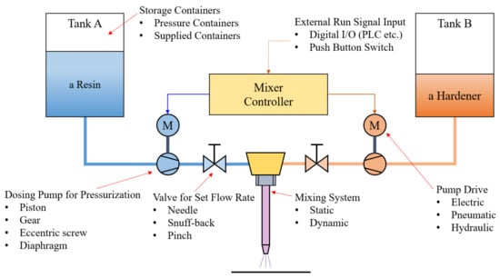
Figure 1.
Schematic diagram of a dosing system for two-part epoxy adhesive (modified from [1]).
On a normal operating state, the mixing ratio mismatch with the suggested value can occur due to an operation error of the mixing system, changing fluid resistance, or the pump or valve operation error that supplies the two adhesive materials. The result will have fatal defects, such as slowed curing time and weakened adhesive strength [1]. However, there are few in-depth studies on these obvious facts [7]. In addition, micro-voids generated during the mixing step reduce adhesion strength [8].
Usually, it takes several to several tens of hours under certain conditions until complete curing, and in a bonding process using epoxy adhesive, the quality of the bonding result can be verified after that. Therefore, if a quality defect in the bonding process is found, all products produced during the curing time are regarded as defective and cause much loss. In order to detect such an error, the flow meters may be mounted on each of the two supplied liquid material pipelines. However, this method may have poor accuracy due to the change in viscosity according to the temperature of the liquid and the change in fluid resistance in the dispensing nozzle and mixer.
1.2. Method for Measuring Material Properties Using an Impedance Measurement Technique
The dielectric constant of a material is based on the difference in the polarizability of ions, which is inherently changed according to the type and amount of the material constituting it. A change in polarizability causes a difference in permittivity. It has various values according to dielectric properties, which are one of the properties of materials. Therefore, it can be used to classify materials [9].
The relative permittivity of material means a value relative to the permittivity of a vacuum. EIS (electrical impedance spectroscopy) technique is a method of measuring the magnitude and phase of impedance that changes according to the input frequency. Through this, the relative permittivity of the dielectric can be obtained indirectly [10].
On the other hand, the impedance characteristics of complex materials have non-linear and complex characteristics in some cases. Therefore, its equivalent electric model and analysis methods have been proposed in various ways [11].
Much research has been performed in various industries, such as mixed solutions [12,13,14,15], biology [16,17,18], food [19], material corrosive evaluation [20], and battery [21,22,23,24,25], as well as the measurement of a chemical reaction using it. Likewise, since various polymer materials including adhesives are also dielectric materials, it can be usefully utilized to measure the properties of epoxy adhesives. Therefore, much research has been performed on this technique [26,27,28,29,30,31]. In addition, a method for monitoring the status of the process online using this has been introduced [17].
1.3. Estimation Method Using Machine Learning
In machine learning, there are regression and classification techniques among supervised learning, clustering in unsupervised learning, and reinforcement learning, selected and applied according to the type of problem.
Among machine learning algorithms, the regression method is used as an inferring method of the result value using the collected data [32,33]. The regression method using machine learning is easier to construct modeling, has better flexibility, and can expect better results compared to using a numerical analysis method for a model with complex equations and non-linear characteristics. Many types of research are being carried out on data processing obtained by machine learning with EIS [34,35,36,37,38]. In addition, research on how to predict the change in permittivity using machine learning has been performed [38,39].
In this study, by applying a regression method among machine learning algorithms, data on impedance according to frequency range at a predetermined mixing ratio and temperature are acquired and learned on a machine learning model. In addition, the performance is confirmed to estimate the mixing ratio of the epoxy using the data on impedance and temperature not used for learning. Furthermore, a developed sensor device and embedded system are applied for the online verification of the mixing ratio’s integrity, which can be used to measure data on a two-part epoxy adhesive process for the learned machine learning model.
As with many studies introduced above, the EIS technique is widely used to estimate material characteristics and aims to find the actual value under various conditions. However, this study aims to detect the different inputs after learning using a machine learning algorithm in known input data and use this for monitoring online. So, an additional resistor was connected in parallel to the electrode plates to suppress the effect of parasitic elements. Moreover, research has been performed to detect variance for monitoring integrity in flowing fluid materials rather than estimating exact impedance values.
2. The Method for the Estimation of the Characteristics for Liquid Materials through Impedance Measurement
2.1. Characteristics of Solutions and Relative Permittivity
To measure the dielectric constant of the material, as shown in Figure 2, a polarization phenomenon is caused by placing a dielectric between two flat electrode plates. Due to this phenomenon, capacitance is generated between the two flat electrode plates, and the magnitude of the capacitance can be expressed as the following Equation (1). A is a flat electrode plate, d is a distance between flat electrode plates, and ε0 is absolute permittivity. C0 is a capacitance when ε0 is 1 that means vacuum between flat electrode plates.
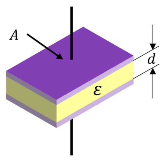
Figure 2.
Dielectric material between two flat electrode plates.
Capacitance (C) is proportional to the relative permittivity (ε) of the dielectric between the two flat electrode plates.
2.2. Relationship between Relative Permittivity and Impedance
By measuring a capacitance as in Equation (1), the relative permittivity can be obtained. As is well known, the relative permittivity has a complex permittivity (ε*) whose characteristics change according to temperature and frequency [9].
Considering the input frequency of the voltage V0 supplied to the two flat electrode plates, it can be expressed as Equation (2). where V is the output voltage and ω means the angular velocity (rad/sec).
In contrast, the actual flowing current can be expressed as Equation (3) below. Where I is the current in a capacitance, Q is the quantity of electric charge.
On the other hand, the relative permittivity can be expressed as a complex value, and as the sum of the real part (ε′) and the imaginary part (ε″), as shown in Equation (4).
Substituting this into Equation (3), the current with respect to the voltage applied to the two flat electrode plates is induced as in Equation (5).
If Ohm’s law is applied to Equation (5), Equation (6) can be obtained for the impedance (Z(ω)) between the two flat electrode plates.
By rearranging Equation (6), it can be expressed as Equation (7) below.
Therefore, the phase difference () in the impedance is as Equation (8).
On the other hand, tan δ is defined as in Equation (9), which is called dielectric loss tangent, and this value is used as a significant indicator to identify the characteristics of materials.
For polymeric materials such as polystyrene and Teflon, ε′ has a value of 2–3, and ε″ has a small value of 0.001 or less [9]. On the other hand, in water, ε′ has a relatively large value of about 80.
In Equations (8) and (9), tan δ is expressed as the phase difference (), as in Equation (10) below.
On the other hand, in Equation (5), the impedance is determined by the sum of the real part and the imaginary part among the dielectric constants having a complex value, and if each of these is separated, it can be expressed as Equation (11) below.
Among them, the imaginary part contributes to the capacitance and the real part contributes to the resistance.
Therefore, the impedance for each component is as shown in Equation (12) below. So, in the two flat electrodes, ε′ and ε″ are the main variables that determine the capacitance and resistance, respectively.
On the other hand, as shown in Figure 3, the above impedance characteristics can be expressed as an equivalent circuit of the parallel connection between the resistor R and the capacitor C.
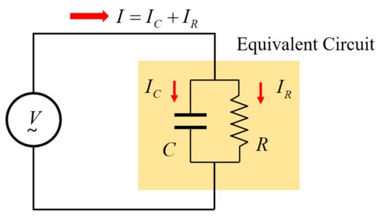
Figure 3.
The equivalent circuit represented to RC parallel connection.
The impedance of the RC parallel circuit can be expressed as Equation (13).
Also, the magnitude and phase difference in the impedance according to the frequency is the same as in Equation (14).
In Equation (13), the output current for the input voltage can be defined using Ohm’s law.
Comparing Equations (11) and (15), R and C are derived as Equations (16) and (17) below.
Equation (15) shows that resistance is determined by ε″. If the change in ε″ is not significant, resistance has a large value when the frequency (ω) is small, and its value decreases in inverse proportion as the frequency increases. In fact, polymeric materials have a very large resistance of several to tens of MΩ at low frequencies, representing the properties of the insulator well. In contrast, capacitance is proportional to ε′ regardless of frequency, as shown in Equation (16). Therefore, the estimation of capacitance can represent the characteristics of ε′ well.
Equations (16) and (17) should be arranged and substitute into Equation (9) to obtain the relationship between tan δ and R, C as shown in Equation (18).
As shown in Equation (14), the phase difference is also matched 1:1 with the magnitude of the impedance. Therefore, tan δ can be defined even by using the magnitude of the impedance. The tangent function has an infinite value when the phase difference () is close to 0° and 0 when it is close to −90°. This means that the ratio of ε′ and ε″ has an enormous difference, and a slight change at this time does not have a significant effect on the phase difference, which is highly disadvantageous for precise measurement of tan δ. Similarly, in the magnitude of the impedance shown in Equation (14), C is almost neglected when the frequency (ω) is close to 0, while R is also practically neglected when the frequency becomes very large. At this time, the phase difference is 0° and −90°, respectively. Considering the characteristics of the tangent function again, the phase difference of −45° is near the cut-off frequency where the values of ε′ and ε″ are almost the same and the magnitude of the impedance decreases by −3 dB. In the vicinity of this frequency, tan δ becomes sensitive to changes in the values of ε′ and ε″.
2.3. Impedance Characteristics of the Parallel RC Circuit
In the RC parallel circuit in Figure 3, the impedance and phase difference can be obtained in the frequency domain using Equation (14), shown in Figure 4. Assuming that R = 10 kΩ and C = 1 μF are initial values, Figure 4a is the result obtained by increasing C by 1 μF, and Figure 4b is the result obtained by increasing R by 10 kΩ. It can be seen that the magnitude of the impedance is sensitive to the change in C in the high-frequency region and sensitive to the change in R in the low-frequency region. At this time, the criterion for dividing the high-frequency region and the low-frequency region is defined as the cut-off frequency (1/RC (rad/sec)). In addition, it can be seen that the change in the phase difference is significant near the frequency.
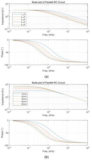
Figure 4.
Bode plots of RC parallel circuit: (a) Change in capacitance (R = 10 kΩ); (b) Change in resistance (C = 1 μF).
Therefore, good results can be expected if an appropriate cut-off frequency is set and tan δ is measured at a frequency near it. In general, the measurement of tan δ in polymer materials is performed at a high frequency of 100 kHz to several GHz or more. One of the reasons is that the resistance value of the polymer material is enormous and causes a high cut-off frequency. Therefore, a change in the phase difference appears at a high frequency, and a change in tan δ is observed. In addition, a significant resistance value at a low frequency may cause a measurement error because the amount of current flowing is very small.
2.4. Effects of Parasitic Elements
Parasitic elements are unintended electrical elements that exist between the electrode plates and the instrument. Figure 5 shows an example. Parasitic resistances RP1 and RP2 occur due to cable resistance and contact resistance of connectors [40]. In addition, the parasitic capacitor (CP) is generated when two wires are long and close to each other. Additionally, parasitic coils (LP1, LP2) are induced when the cable is twisted. The configuration of a complex circuit network causes many errors, even in the frequency response. Since the parasitic resistance is very small compared to the resistance of the electrode plates at low frequency, the effect is also minimal. However, at a high frequency, the resistance of the electrode plates also becomes small, so it is necessary to be careful. Even if the parasitic capacitor has a constant value, it acts as a capacitance measurement error. The impedance due to the parasitic coil increases according to the frequency increases, causing many errors at high frequency; therefore, if the measurement frequency is carried out in a relatively low-frequency range, the effect of the parasitic elements can be minimized. Therefore, the selection of a moderately low cut-off frequency is advantageous for impedance measurement.
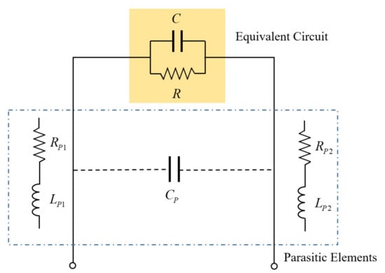
Figure 5.
Parallel RC circuit with parasitic elements.
2.5. Connection of Additional Resistor
As mentioned above, it is most advantageous to measure tan δ near the cut-off frequency. However, since cured epoxy with insulator properties has a significant resistance, a cut-off frequency is generated at a very high frequency. Moreover, measurements at high frequencies have several disadvantages.
Figure 6 shows a circuit in which an additional resistor, Ra (10 kΩ), is connected in parallel with the two flat electrodes.
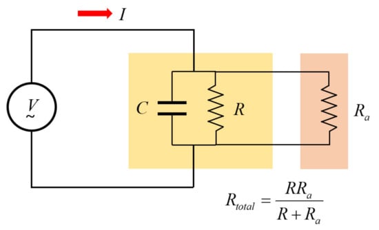
Figure 6.
Parallel RC circuit with additional resistors connected.
Ra is more than 100 times smaller than R at low frequencies and the parallel resistance composed of R and Ra induces more complex non-linear characteristics as shown in Figure 7. For example, when R is 1 MΩ and Ra is 10 kΩ, the total resistance becomes 9.901 kΩ according to the parallel connection formula of resistors, and when it is 10 MΩ, the total resistance becomes 9.90 kΩ. Therefore, it has the effect of changing a change of 1 to 10 MΩ into a change of 89 Ω, so it has non-linearity and is very insensitive to the change of ε″. However, there is an advantage that the cut-off frequency of the impedance equivalent circuit can be adjusted from a high frequency to a low frequency. This has the effect of significantly reducing the error caused by parasitic elements at high frequencies.
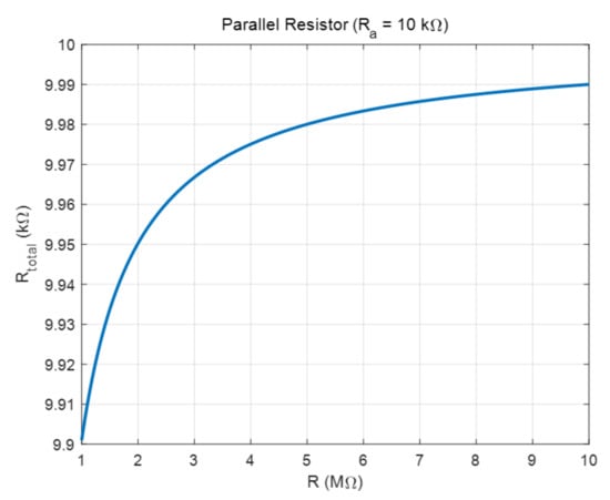
Figure 7.
Change in resistance of the two plate electrodes and change in total resistance.
In general, in the case of polymer materials, ε″ has a size that is very small compared to ε′ [9]. Additionally, the purpose of this study is not to accurately evaluate the relative permittivity but to measure the impedance with a small error and to estimate the change in the mixing ratio as the change in the impedance. Therefore, it was possible to obtain the desired result without considering the effect due to the additional resistance.
3. Experimental Device Configuration and Results
3.1. Configuration of the Impedance Measurement Circuit
There are various methods for measuring impedance, such as the bridge method, the I-V method, and the auto-balancing bridge method [40].
In this study, the auto-balancing bridge method shown in Figure 8 was applied. In this method, a sine wave voltage signal (Vx(ω)) of varying frequency is input to an unknown RLC network, and the current I(ω) flowing at this time is converted into a voltage Vo(ω) using an I-V converter. It can be applied to a wide range of frequencies from 20 Hz to 120 MHz, and has the advantage of high precision compared to other methods.
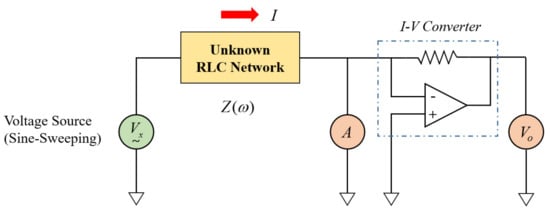
Figure 8.
Diagram of an auto-balancing bridge method.
Impedance is measured as Equation (19) below according to Ohm’s Law.
For this system development, the AD5934 with I2C communication, a component for impedance measurement by Analog Device Inc., was used. It sweeps the input frequency within a specific range, collects the data of the output voltage, and applies the DFT (Discrete Fourier Transform) algorithm to obtain the magnitude and phase difference in the impedance for each frequency.
3.2. Impedance Change According to Temperature Change
The relative permittivity tends to change highly according to temperature because the polarizability changes according to the molecule’s activity [9]. Therefore, it is essential to consider temperature when measuring impedance. In addition, two-part epoxy adhesive starts a chemical reaction from the moment it is mixed, causing an increase in temperature. Therefore, it is necessary to measure temperature change and impedance, collect the data, and use it for analysis. In this study, RTD was used for temperature measurement. The RTD is a sensor element whose resistance value changes precisely according to a change in temperature. The MAX31865 was used for temperature data acquisition using an RTD. It converts the resistance value of the RTD into temperature data and transmits it through SPI communication.
Figure 9 shows the structure of the impedance measuring device developed in this study. A Raspberry Pi, which is often used as an IoT device with the internet connection, was used for data collection using I2C and SPI communication and execution of machine learning algorithms.
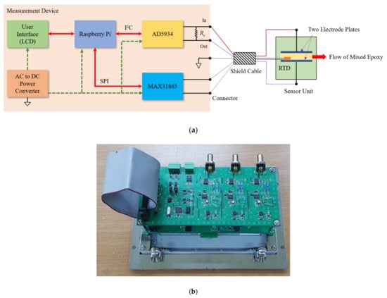
Figure 9.
Impedance measurement board with Raspberry Pi: (a) Block diagram; (b) A picture of the developed device.
3.3. Design of Sensor Structure for Impedance Measurement
Two plate electrodes can be easily manufactured using a PCB pattern. A copper plate 76 μm thickness was attached to the surface and was coated thinly with a PSR (Photo imageable Solder Resist) ink. PSR ink is known to use epoxy-based materials to prevent soldering on unwanted parts. Figure 10 shows the feature and dimension of electrodes with bolt halls for fixing to the sensor body, through-halls for wire soldering, and a pad for mounting RTD. The specification of the RTD is that size is 1.6 × 3.25 × 0.9 mm (SMD size 1206), R0 is 1000 Ω, and resistance tolerance is ±0.12%.
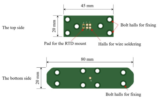
Figure 10.
Drawing of the two plate electrodes using a PCB pattern.
A sensor with the structure shown in Figure 11 was designed. In addition, it was designed to be inserted in the middle of the pipe through which the mixed epoxy flows. The sensor body was made of PTEF material and sealed with an O-ring. Figure 12 shows the photo of the actually fabricated sensor device.
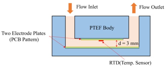
Figure 11.
Basic structure of impedance sensor for epoxy flow.
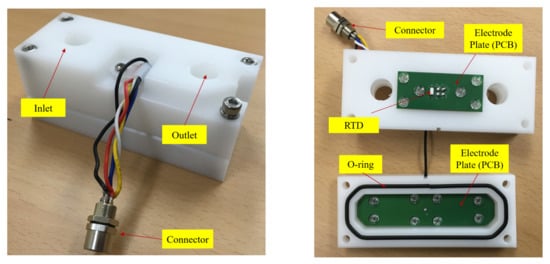
Figure 12.
Design of impedance sensor with RTD.
Air, a resin, and a hardener were injected into the manufactured sensor at 20.2 °C, and capacitance was measured at a frequency of 1 kHz to 20 kHz using an LCR meter. The relative permittivity according to frequency was obtained by dividing the capacitance of a resin and a hardener by the capacitance of air. It can be seen that there is a sharp change at frequencies below 5 kHz, as shown in Figure 13.
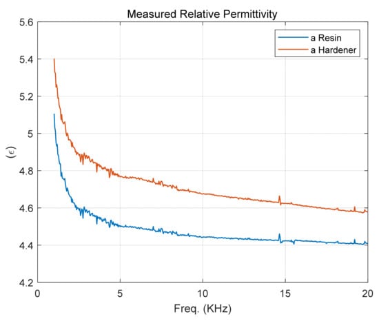
Figure 13.
Measured relative permittivity of a resin and a hardener at 20.2 °C.
3.4. Composition of Two-Part Epoxy Adhesive Mixing Experiment Equipment
Various mixing and dispensing systems such as manual cartridge gun are used in the industry that actually uses two-part epoxy adhesive. A dosing system is also used to configure an automated process as shown in Figure 1. The dosing system stores each liquid material in two tanks and uses two pumps to discharge the continuous supply according to the mixing ratio and to execute mixing in the mixer device.
Mixing ratio errors can occur for various reasons, such as a pump setting mistake, change in viscosity according to temperature, and abnormal control operation. In this study, a two-part epoxy adhesive mixing device, as shown in Figure 14, was used for experiments and data collection using an accurate mixing ratio. In addition, this device has two tanks, each for storing the resin and hardener of two-part epoxy adhesive. It has two replaceable cylinders, and the mixing ratio is determined by replacing cylinders with different volumes. The maximum discharge volume of cylinders is 40 cc, and the fluid velocity at the sensor is about 0.4~0.6 m/s, depending on the air pressure setting. The two liquid materials are discharged by moving forward at the same time according to the compressed air supplied to the air cylinder. Therefore, continuous feeding is impossible, but the correct mixing ratio is maintained. The developed impedance sensor is inserted between the mixer and the dispenser to collect impedance and temperature data of the mixed adhesive.
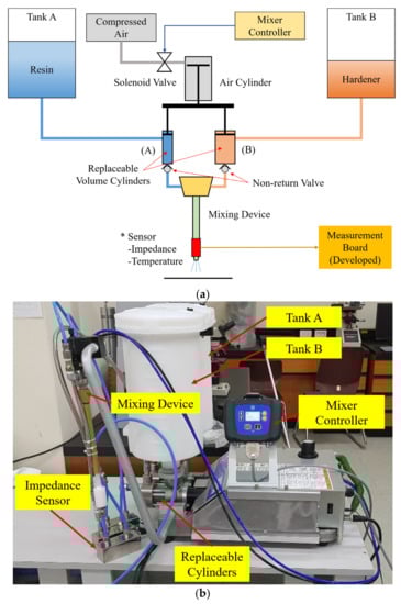
Figure 14.
The composition of the experimental device: (a) Fixed ratio two-part epoxy adhesive mixing device with sensor; (b) A picture of the experimental device.
3.5. Experimental Progress and Analysis of Result Data
Experiments were conducted while changing the mixing ratio by preparing cylinders of various ratios. It can be expected that two-part epoxy adhesive will be cured at the moment it is mixed, and its physical properties will continue to change over time. The two-part epoxy adhesive used in the experiment had a curing time of 24 h, and the measurement was made immediately after mixing, so it was judged that the error according to the curing time was very short.
The average graph of five times the measurement for the three ratios among the frequency response data of impedance is shown in Figure 15a. The mixing ratio was expressed in % of the ratio of the hardener to the resin. The experiment was measured in the frequency range of 1 kHz to 50 kHz. In addition, the section that was significantly non-linear due to parasitic factors with little change was removed, and the section from 5 kHz to 15 kHz was used for analysis.
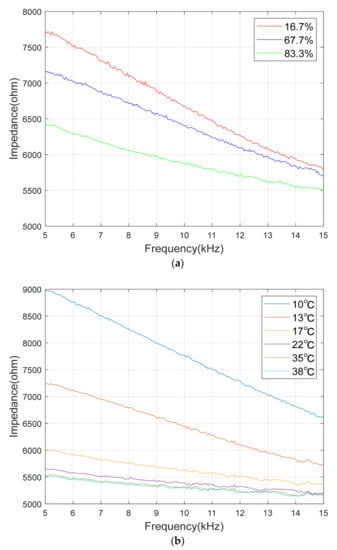
Figure 15.
Measured impedance graph: (a) Impedance graph by different mixture ratio at 13 °C; (b) Impedance graph by different temperatures.
The AD5934, a component for impedance measurement, can obtain impedance data with a frequency resolution of 0.1 Hz or less. However, if the frequency resolution is too small within the set frequency range, it takes much time to collect data. Moreover, the lower the frequency occurs, the longer the measurement time, because that lower frequency needs a long time for one period in the time domain. It seems that using a large number of frequency data among the training data for machine learning will improve to obtain high accuracy. However, it is difficult to obtain homogeneous data because a long measurement time causes a change in impedance according to the progress of the chemical reaction. Therefore, it is necessary to set a short data collection time to obtain homogeneous data. In this study, 51 pieces of data are extracted at intervals of 200 Hz between 5 kHz and 15 kHz in the frequency domain. The data collection time takes about 0.6 s, which is very short compared to the entire curing time of the two-part epoxy adhesive used in this experiment.
From this, it can be seen that as the frequency of the input sine wave increases, as with the capacitance characteristic of the RC circuit, the impedance decreases significantly. In addition, it can be seen that the magnitude of the mixed adhesive decreases as the mixing ratio increases. In other words, it can be seen that the mixing ratio induces a significant change in capacitance. That is, the mixed adhesive has a significant change in ε’ according to the mixing ratio.
3.6. Impedance Change with Temperature Change
In order to measure the change in impedance according to the temperature change, the sensor containing the mixed adhesive was completely sealed, and then the temperature and the impedance were measured by increasing the temperature of the adhesive using a cold and hot water bath. The temperature change experiment used the measurement value of RTD inside the sensor, and the impedance was measured while changing the temperature in the range of 10 °C to 40 °C. Figure 15b shows the impedance data with respect to the temperature change for the mixed adhesive with a mixing ratio of 67.7%. It can be seen that the magnitude of the impedance decreases as the temperature increases, but when the temperature increases over a certain level, the slope change is not significant.
4. Mixing Ratio Estimation Using Machine Learning Algorithm
4.1. Data Preprocessing for Machine Learning
As a method for estimating the ratio of the mixed adhesive, the parameters of the governing equation may be determined using a regression analysis technique such as the least square method, and the measured result may be estimated by the interpolation method. However, as shown above, impedance has a non-linear characteristic and is sensitive to temperature. Therefore, when estimating the mixing ratio using this algorithm, an error is expected to be very large. Thus, a deep learning model was created to perform robust prediction despite non-linear changes according to frequency and temperature changes, and mixing ratio prediction was performed using this.
A significant amount of training data is required to learn a deep learning algorithm. However, since the number of cylinder volumes of the experimental apparatus is limited, it is complicated to collect data according to precise changes in various mixing ratios. For that reason, virtual data were created based on the measured data to confirm the usability of this device.
First, the impedance value for each frequency according to the mixing ratio was changed to the impedance of the mixing ratio when the frequency was changed at an interval of 500 Hz. Next, curve fitting was applied to generate virtual data for various mixed ratios. The generated virtual data is shown in Figure 16a.
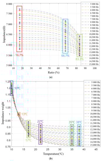
Figure 16.
Modified impedance graph and impedance weight graph: (a) Estimated impedance by each frequency; (b) Impedance weight by each frequency.
In addition, it is also necessary to generate virtual data on the change in impedance for temperature change. Therefore, the impedance data for each frequency according to temperature was converted into impedance weight data for each temperature according to frequency. The impedance change according to the mixing ratio was determined by setting the impedance weight of 13 °C to 1. After calculating the weights at different temperatures, by applying their curve fitting, virtual data about temperature can be created as shown in Figure 16b.
With the two types of data above, one mixing ratio can be expressed as one curved surface in a three-dimensional space. In Figure 17, one curved surface represents the impedance according to temperature and frequency at the same mixing ratio. And each curved surface represents a value obtained by dividing the mixing ratio between 16.7% and 83.3% into 10 equal parts, and the lower the mixing ratio, the higher the impedance value in the upper layer. It can also be seen that the lower the temperature and the lower the frequency, the higher the impedance magnitude. The generated data were used for the training and testing of the deep learning model. A large number of datasets are required for the excellent performance of machine learning. Therefore, it is necessary to extract an appropriate amount of data from the surfaces shown in Figure 17. For the machine learning training dataset, 51 impedance data according to frequency, 100 mixing ratio data, and 100 temperature data were extracted and used for learning.
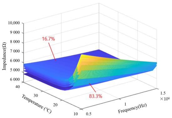
Figure 17.
Impedance with temperature and frequency represented 3D surface form.
4.2. Training and Evaluation of Machine Learning Models
Various algorithms exist in machine learning. In this study, the problem of finding an appropriate output for an input is a regression during supervised learning. For this purpose, an ANN (Artificial Neural Network) [41], as shown in Figure 18, was constructed using the tensor flow package in an embedded Linux environment. The number of input layer nodes of the ANN model used has 52 nodes, including one temperature data and impedance magnitude for 51 frequencies. Furthermore, the output layer has only one node to predict the mixing ratio.
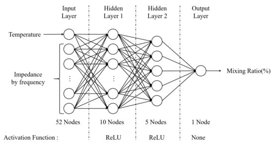
Figure 18.
The ANN model with activation function for regression.
The number of hidden layers and the number of nodes can be set arbitrarily, and accordingly, the learning time and the accuracy of the results vary greatly. The composition and number of hidden layers used in this study and their respective activation functions are shown in Figure 18.
The ANN model was learned by selecting 75% of the prepared data as training data with gradient descent, and as shown in Figure 18, it was confirmed that the loss decreased and convergence as the number of learning increased as shown in Figure 19. Table 1 shows some of the results for inputting test data not used for training to the learned ANN model. As a result of calculating the difference between the actual mixing ratio and the predicted mixing ratio, the difference is within 0.74%, so it can be confirmed that the model is well trained and outputs show excellent results.
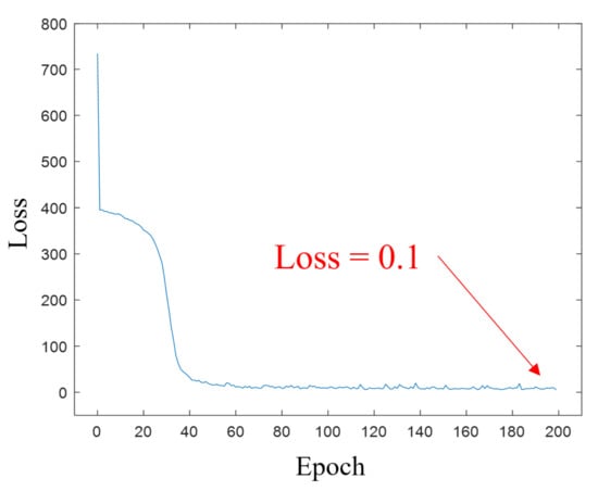
Figure 19.
Loss with epoch number graph.

Table 1.
Test result of the learned ANN model.
4.3. A Suggestion for Configuring a Remote Online Monitoring System
As with the introduced mixing ratio of two-part epoxy adhesives in this study, the integrity of the liquid can be verified through impedance monitoring. By applying this, the fluid’s integrity of various processes can be effectively monitored. For example, solutions used for cleaning and coating in semiconductor and display manufacturing processes require high integrity.
Since the developed system uses an IoT device (Raspberry Pi), it can easily connect to the network. Thus, it is possible to configure a system that remotely verifies the integrity of various liquids such as epoxy, solutions, and oils [42]. Figure 20 shows a flow chart of the suggested software structure to configure it. The software has three modes: a learning mode for machine learning, a testing mode for online testing and monitoring, and a stop mode for termination. The ANN model is learned in the learning mode after setting the label value for the acquired impedance and temperature data. In the case of two-part epoxy adhesives, the mixing ratio corresponds to the label value. At this time, it is assumed that the liquid flowing through the sensor is in integrity. When sufficient learning has progressed, the mode is changed to testing mode. In this mode, impedance and temperature data of the liquid flowing through the sensor are input to the learned ANN, and the result is estimated. The difference between the set label value and the estimated value becomes an error. If the absolute value of error is greater than δ, it is judged that the impaired integrity and an alarm is issued. The online remote monitoring system can be configured by transmitting the evaluation results to a network-connected remote monitoring server [43].
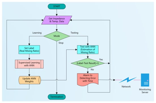
Figure 20.
Suggested flow chart to configure for an online remote liquid monitoring system.
5. Conclusions
In this study, the correlation between the mixing ratio and the dielectric constant of the two-part epoxy adhesive was experimentally verified. In addition, the sensor was designed and manufactured, which can be inserted into a liquid pipe for measuring the impedance and temperature of liquids involving two-part epoxy adhesives. In addition, with the EIS technique, an embedded system and measurement circuits were constructed that can measure temperature and impedance by frequency. Using this, impedance and temperature measurements were performed under various mixing ratios and temperature conditions.
Based on the measured data, curve fitting was applied to the mixing ratio and temperature to generate virtual data. Then, an ANN model was learned using arbitrarily selected training data, and the performance of the learned model was verified using the test data. As a result of the test, the excellent estimation performance of the learned model was confirmed.
The advantage of the machine learning algorithm is that it is possible to check the integrity of the mixing ratio using experimental data without knowing strictly the properties of complex polymer materials and changes in properties that occur during curing, including micro-voids in the mixed epoxy. Therefore, monitoring these changes can be helpful in evaluating their integrity. As a disadvantage, many new data are required whenever the composition or mixing ratio of a two-part epoxy adhesive is changed; though, this is when applied to an actual process. However, if many data are collected and learned in a steady state, the occurrence of defects can be alarmed in near real-time.
In order to monitor the mixing ratio of epoxy in actual industrial sites, a flow meter is often inserted into the pipe at both ends of the mixing system to which each fluid material is supplied in the dosing system of Figure 1. It measures the flow rate through two pipes and can know the mixing ratio through a simple calculation. On the other hand, there are several disadvantages. The flow meter structure is complicated, and it is integrated with the measuring device, so it is expensive and requires two sensors for measuring the mixing ratio. Furthermore, cleaning work is needed for reuse when changing the dispensing process. This method estimates the mixing ratio by measuring the flow rate before mixing and does not directly represent the results for the mixed epoxy. In contrast, the result for this study can estimate the characteristics of the mixed epoxy by using a single sensor. Since the sensor structure is simple, only the sensor can be separated and replaced without reusing it. Thus, maintenance cost is cheaper than applying the flow meter. Moreover, it has a wide range of applications by essentially measuring the characteristic of materials
In addition, it is expected that this developed device can be easily used as an IoT remote liquid monitoring system because a Raspberry Pi has a network function such as the internet protocol (TCP/IP). Moreover, it can be applied widely to process fields using fluids, such as various chemical processes, beverage production, oil refining, and wastewater disposal.
Author Contributions
Conceptualization, C.H.A.; methodology, C.H.A.; data processing, C.H.A. and J.H.C.; machine learning programming, J.H.C. All authors have read and agreed to the published version of the manuscript.
Funding
This paper was supported by the education and research promotion program of KOREATECH in 2020; These results were supported by “Regional Innovation Strategy (RIS)” through the National Research Foundation of Korea (NRF) funded by the Ministry of Education (MOE) (2021RIS-004).
Institutional Review Board Statement
Not applicable.
Informed Consent Statement
Not applicable.
Data Availability Statement
Data are contained within the article.
Conflicts of Interest
The authors declare no conflict of interest.
References
- Da Silva, L.F.M.; Ochsner, A.; Adams, R.D. Handbook of Adhesion Technology; Springer: Berlin/Heidelberg, Germany, 2011; Volume 1. [Google Scholar]
- Lakshmi, B.; Shivananda, K.N.; Mahendra, K.N. Synthesis, Characterization and Curing Studies of Thermosetting Epoxy Resin with Amines. Bull. Korean Chem. Soc. 2010, 31, 2272–2278. [Google Scholar] [CrossRef][Green Version]
- Antelo, J.; Akhavan-Safar, A.; Carbas, R.J.C.; Marques, E.A.S.; Goyal, R.; da Silva, L.F.M. Replacing Welding with Adhesive Bonding: An Industrial Case Study. Int. J. Adhes. Adhes. 2022, 113, 103064. [Google Scholar] [CrossRef]
- Akhavan-Safar, A.; Ramezani, F.; Delzendehrooy, F.; Ayatollahi, M.R.; da Silva, L.F.M. A Review on Bi-Adhesive Joints: Benefits and Challenges. Int. J. Adhes. Adhes. 2022, 114, 103098. [Google Scholar] [CrossRef]
- Weißgraeber, P.; Becker, W. Finite Fracture Mechanics Model for Mixed Mode Fracture in Adhesive Joints. Int. J. Solids Struct. 2013, 50, 2383–2394. [Google Scholar] [CrossRef]
- De La Pierre, S.; Scalici, T.; Tatarko, P.; Valenza, A.; Goglio, L.; Paolino, D.S.; Ferraris, M. Torsional Shear Strength and Elastic Properties of Adhesively Bonded Glass-to-Steel Components. Mater. Des. 2020, 192, 108739. [Google Scholar] [CrossRef]
- Liu, Y.; Gu, Z.; Hughes, D.J.; Ye, J.; Hou, X. Understanding Mixed Mode Ratio of Adhesively Bonded Joints Using Genetic Programming (GP). Compos. Struct. 2021, 258, 113389. [Google Scholar] [CrossRef]
- Katnam, K.B.; Stevenson, J.P.J.; Stanley, W.F.; Buggy, M.; Young, T.M. Tensile Strength of Two-Part Epoxy Paste Adhesives: Influence of Mixing Technique and Micro-Void Formation. Int. J. Adhes. Adhes. 2011, 31, 666–673. [Google Scholar] [CrossRef]
- Young, R.J.; Lovell, P.A. Introduction to Polymers, 3rd ed.; CRC Press: Boca Raton, FL, USA, 2011. [Google Scholar]
- Chang, B.-Y.; Park, S.-M. Electrochemical Impedance Spectroscopy. Annu. Rev. Anal. Chem. 2010, 3, 207–229. [Google Scholar] [CrossRef]
- Choi, W.; Shin, H.-C.; Kim, J.M.; Choi, J.-Y.; Yoon, W.-S. Modeling and Applications of Electrochemical Impedance Spectroscopy (EIS) for Lithium-Ion Batteries. J. Electrochem. Sci. Technol. 2020, 11, 1–13. [Google Scholar] [CrossRef]
- Mandalunis, S.; Sorichetti, P.A.; Romano, S.D. Relative Permittivity of Bioethanol, Gasoline and Blends as a Function of Temperature and Composition. Fuel 2021, 293, 120419. [Google Scholar] [CrossRef]
- Husairi, F.S.; Rouhi, J.; Eswar, K.A.; Ooi, C.H.R.; Rusop, M.; Abdullah, S. Ethanol Solution Sensor Based on ZnO/PSi Nanostructures Synthesized by Catalytic Immersion Method at Different Molar Ratio Concentrations: An Electrochemical Impedance Analysis. Sens. Actuators A Phys. 2015, 236, 11–18. [Google Scholar] [CrossRef]
- Lima, L.F.; Vieira, A.L.; Mukai, H.; Andrade, C.M.G.; Fernandes, P.R.G. Electric Impedance of Aqueous KCl and NaCl Solutions: Salt Concentration Dependence on Components of the Equivalent Electric Circuit. J. Mol. Liq. 2017, 241, 530–539. [Google Scholar] [CrossRef]
- Ghasemi, S.; Darestani, M.T.; Abdollahi, Z.; Hawkett, B.S.; Gomes, V.G. Electrical Impedance Spectroscopy for Determining Critical Micelle Concentration of Ionic Emulsifiers. Colloids Surf. A Physicochem. Eng. Asp. 2014, 441, 195–203. [Google Scholar] [CrossRef]
- Calvo, P.C.; Campo, O.; Guerra, C.; Castaño, S.; Fonthal, F. Design of Using Chamber System Based on Electrical Impedance Spectroscopy (EIS) to Measure Epithelial Tissue. Sens. Bio-Sens. Res. 2020, 29, 100357. [Google Scholar] [CrossRef]
- Sarró, E.; Lecina, M.; Fontova, A.; Solà, C.; Gòdia, F.; Cairó, J.J.; Bragós, R. Electrical Impedance Spectroscopy Measurements Using a Four-Electrode Configuration Improve on-Line Monitoring of Cell Concentration in Adherent Animal Cell Cultures. Biosens. Bioelectron. 2012, 31, 257–263. [Google Scholar] [CrossRef]
- Tura, A.; Sbrignadello, S.; Barison, S.; Conti, S.; Pacini, G. Impedance Spectroscopy of Solutions at Physiological Glucose Concentrations. Biophys. Chem. 2007, 129, 235–241. [Google Scholar] [CrossRef]
- Grossi, M.; Lanzoni, M.; Pompei, A.; Lazzarini, R.; Matteuzzi, D.; Riccò, B. Detection of Microbial Concentration in Ice-Cream Using the Impedance Technique. Biosens. Bioelectron. 2008, 23, 1616–1623. [Google Scholar] [CrossRef]
- Encinas-Sánchez, V.; de Miguel, M.T.; Lasanta, M.I.; García-Martín, G.; Pérez, F.J. Electrochemical Impedance Spectroscopy (EIS): An Efficient Technique for Monitoring Corrosion Processes in Molten Salt Environments in CSP Applications. Sol. Energy Mater. Sol. Cells 2019, 191, 157–163. [Google Scholar] [CrossRef]
- Kuipers, M.; Schröer, P.; Nemeth, T.; Zappen, H.; Blömeke, A.; Sauer, D.U. An Algorithm for an Online Electrochemical Impedance Spectroscopy and Battery Parameter Estimation: Development, Verification and Validation. J. Energy Storage 2020, 30, 101517. [Google Scholar] [CrossRef]
- Kim, J.; Krüger, L.; Kowal, J. On-Line State-of-Health Estimation of Lithium-Ion Battery Cells Using Frequency Excitation. J. Energy Storage 2020, 32, 101841. [Google Scholar] [CrossRef]
- Zhou, X.; Huang, J. Impedance-Based Diagnosis of Lithium Ion Batteries: Identification of Physical Parameters Using Multi-Output Relevance Vector Regression. J. Energy Storage 2020, 31, 101629. [Google Scholar] [CrossRef]
- Tran, M.L.; Fu, C.-C.; Wu, M.-H.; Juang, R.-S. Experimental Verification on Real-Time Fouling Analysis in Crossflow UF of Protein Solutions by Electrical Impedance Spectroscopy. J. Taiwan Inst. Chem. Eng. 2022, 133, 104197. [Google Scholar] [CrossRef]
- Shu, X.; Shen, S.; Shen, J.; Zhang, Y.; Li, G.; Chen, Z.; Liu, Y. State of Health Prediction of Lithium-Ion Batteries Based on Machine Learning: Advances and Perspectives. iScience 2021, 24, 103265. [Google Scholar] [CrossRef] [PubMed]
- Drozdov, A.D.; deClaville Christiansen, J. Modeling Dielectric Permittivity of Polymer Composites at Microwave Frequencies. Mater. Res. Bull. 2020, 126, 110818. [Google Scholar] [CrossRef]
- Akbaş, H.Z.; Durmuş, H.; Ahmetlï, G. Dielectric properties of cured epoxy with teta. Ozean J. Appl. Sci. 2009, 2, 443–449. [Google Scholar]
- Pan, M.; Zhang, C.; Liu, B.; Mu, J. Dielectric and Thermal Properties of Epoxy Resin Nanocomposites Containing Polyhedral Oligomeric Silsesquioxane. JMSR 2012, 2, 153. [Google Scholar] [CrossRef][Green Version]
- Hussain, W.A.; Hussein, A.A.; Khalaf, J.M.; Al-Mowali, A.H.; Sultan, A.A. Dielectric Properties and a.c. Conductivity of Epoxy/Alumina Silicate NGK Composites. ACES 2015, 5, 282–289. [Google Scholar] [CrossRef]
- Wang, Q.; Chen, G. Effect of Nanofillers on the Dielectric Properties of Epoxy Nanocomposites. Adv. Mater. Res. 2012, 1, 93–107. [Google Scholar] [CrossRef]
- Mujahid, M.; Srivastava, D.S.; Avasthi, D.K. Dielectric Constant and Loss Factor Measurement of Polycarbonate, Makrofol KG Using Swift Heavy Ion O5+. Radiat. Phys. Chem. 2011, 80, 582–586. [Google Scholar] [CrossRef]
- Iban, M.C.; Şentürk, E. Machine Learning Regression Models for Prediction of Multiple Ionospheric Parameters. Adv. Space Res. 2022, 69, 1319–1334. [Google Scholar] [CrossRef]
- Narayanan, S.S.S.; Thangavel, S. Machine Learning-Based Model Development for Battery State of Charge-Open Circuit Voltage Relationship using Regression Techniques. J. Energy Storage 2022, 49, 104098. [Google Scholar] [CrossRef]
- Zhu, S.; Sun, X.; Gao, X.; Wang, J.; Zhao, N.; Sha, J. Equivalent Circuit Model Recognition of Electrochemical Impedance Spectroscopy via Machine Learning. J. Electroanal. Chem. 2019, 855, 113627. [Google Scholar] [CrossRef]
- Liu, J.; Ciucci, F. The Gaussian Process Distribution of Relaxation Times: A Machine Learning Tool for the Analysis and Prediction of Electrochemical Impedance Spectroscopy Data. Electrochim. Acta 2020, 331, 135316. [Google Scholar] [CrossRef]
- Shohan, S.; Harm, J.; Hasan, M.; Starly, B.; Shirwaiker, R. Non-Destructive Quality Monitoring of 3D Printed Tissue Scaffolds via Dielectric Impedance Spectroscopy and Supervised Machine Learning. Procedia Manuf. 2021, 53, 636–643. [Google Scholar] [CrossRef]
- Bongiorno, V.; Gibbon, S.; Michailidou, E.; Curioni, M. Exploring the Use of Machine Learning for Interpreting Electrochemical Impedance Spectroscopy Data: Evaluation of the Training Dataset Size. Corros. Sci. 2022, 198, 110119. [Google Scholar] [CrossRef]
- Chen, L.; Kim, C.; Batra, R.; Lightstone, J.P.; Wu, C.; Li, Z.; Deshmukh, A.A.; Wang, Y.; Tran, H.D.; Vashishta, P.; et al. Frequency-Dependent Dielectric Constant Prediction of Polymers Using Machine Learning. npj Comput. Mater. 2020, 6, 61. [Google Scholar] [CrossRef]
- Jang, D.; Kil, T.; Yoon, H.N.; Seo, J.; Khalid, H.R. Artificial Neural Network Approach for Predicting Tunneling-Induced and Frequency-Dependent Electrical Impedances of Conductive Polymeric Composites. Mater. Lett. 2021, 302, 130420. [Google Scholar] [CrossRef]
- A Guide to Measurement Technology and Techniques, 4th ed.; Agilent Technologies: Santa Clara, CA, USA, 2013.
- Zafar, M.; Aggarwal, A.; Rene, E.R.; Barbusiński, K.; Mahanty, B.; Behera, S.K. Data-Driven Machine Learning Intelligent Tools for Predicting Chromium Removal in an Adsorption System. Processes 2022, 10, 447. [Google Scholar] [CrossRef]
- Reis, M.S.; Gins, G. Industrial Process Monitoring in the BigData/Industry 4.0 Era: From Detection, to Diagnosis, to Prognosis. Processes 2017, 5, 35. [Google Scholar] [CrossRef]
- Kuo, Y.-W.; Wen, W.-L.; Hu, X.-F.; Shen, Y.-T.; Mia, S.-Y. A LoRa-Based Multisensor IoT Platform for Agriculture Monitoring and Submersible Pump Control in a Water Bamboo Field. Processes 2021, 9, 813. [Google Scholar] [CrossRef]
Publisher’s Note: MDPI stays neutral with regard to jurisdictional claims in published maps and institutional affiliations. |
© 2022 by the authors. Licensee MDPI, Basel, Switzerland. This article is an open access article distributed under the terms and conditions of the Creative Commons Attribution (CC BY) license (https://creativecommons.org/licenses/by/4.0/).