
A Techno-Economic Assessment of Fischer–Tropsch Fuels Based on Syngas from Co-Electrolysis

 , , , ,
Abstract
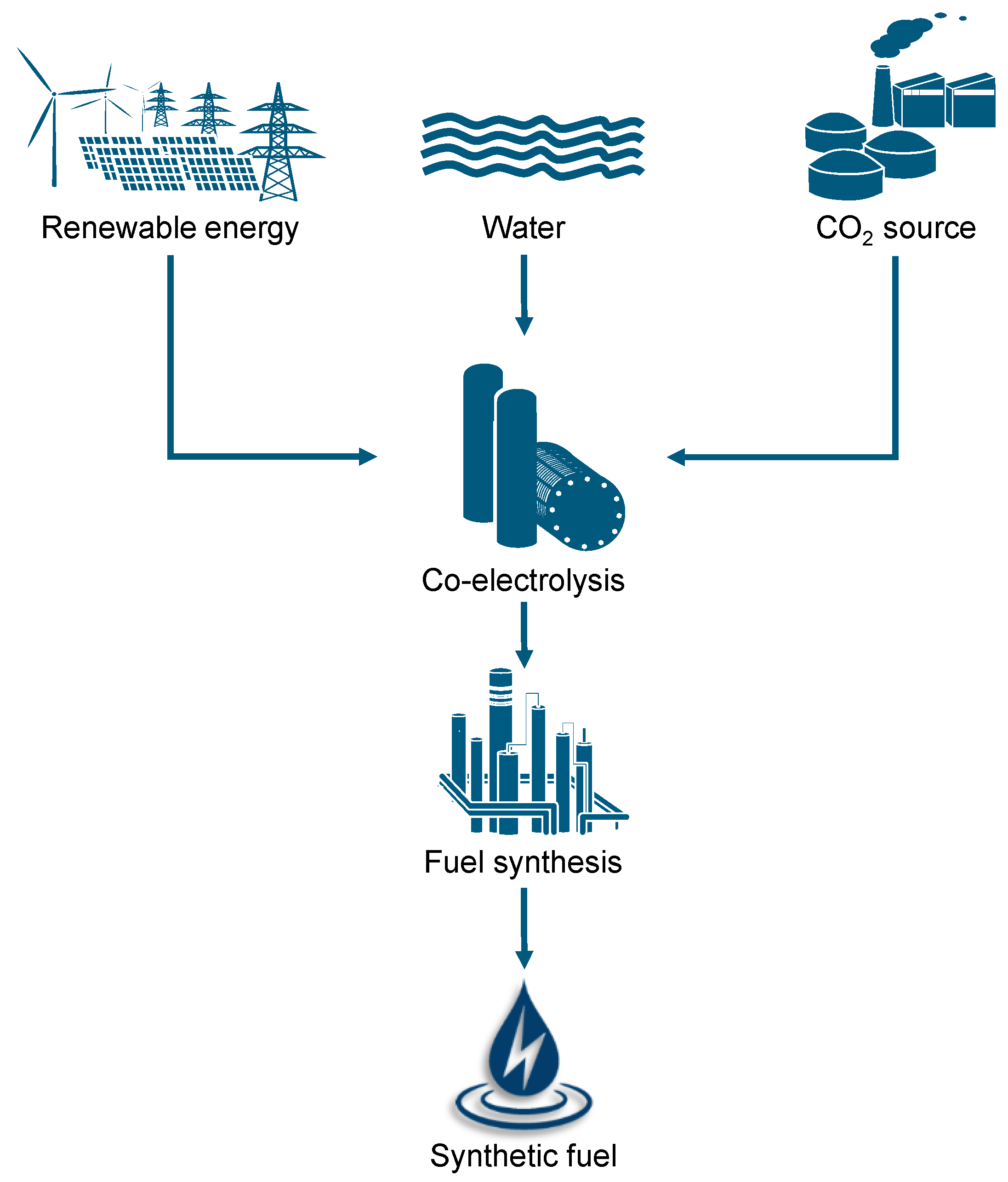
:1. Introduction
- Section 2 provides some insights into the motivation to apply power-to-fuel processes. An overview of already implemented and future planned power-to-liquid or power-to-fuel projects is given.
- Section 3 explains the basics of the individual components used in the developed power-to-fuel process. At the end, the degree of technological maturity of the individual components of the developed fuel synthesis is examined.
- The topic of Section 4 is the development and design of the selected power-to-fuel process. For this purpose, the more precise framework conditions and resulting structure of the fuel synthesis are presented first. Then, the modeling and simulation of the process in Aspen Plus is explored.
- Section 5 presents and discusses the results of the process analysis simulations. First, it is determined whether the fuels produced meet all of the requirements and then the material and energy balance of the process is examined. Finally, based on the efficiency, an energetic comparison between the developed fuel synthesis and alternative power-to-liquid processes is carried out.
- Section 6 analyzes the economic aspects of the developed power-to-fuel process. First, the manufacturing costs of the fuels produced are determined. Then, the influence of various factors on the production costs is examined through a sensitivity analysis. Finally, the production costs of the developed fuel synthesis route are compared with those of alternative power-to-liquid processes.
- In Section 7, the results of the work are summarized and an outlook on the main research areas are given.
2. Background
3. Basic Process Units of PtF System Design
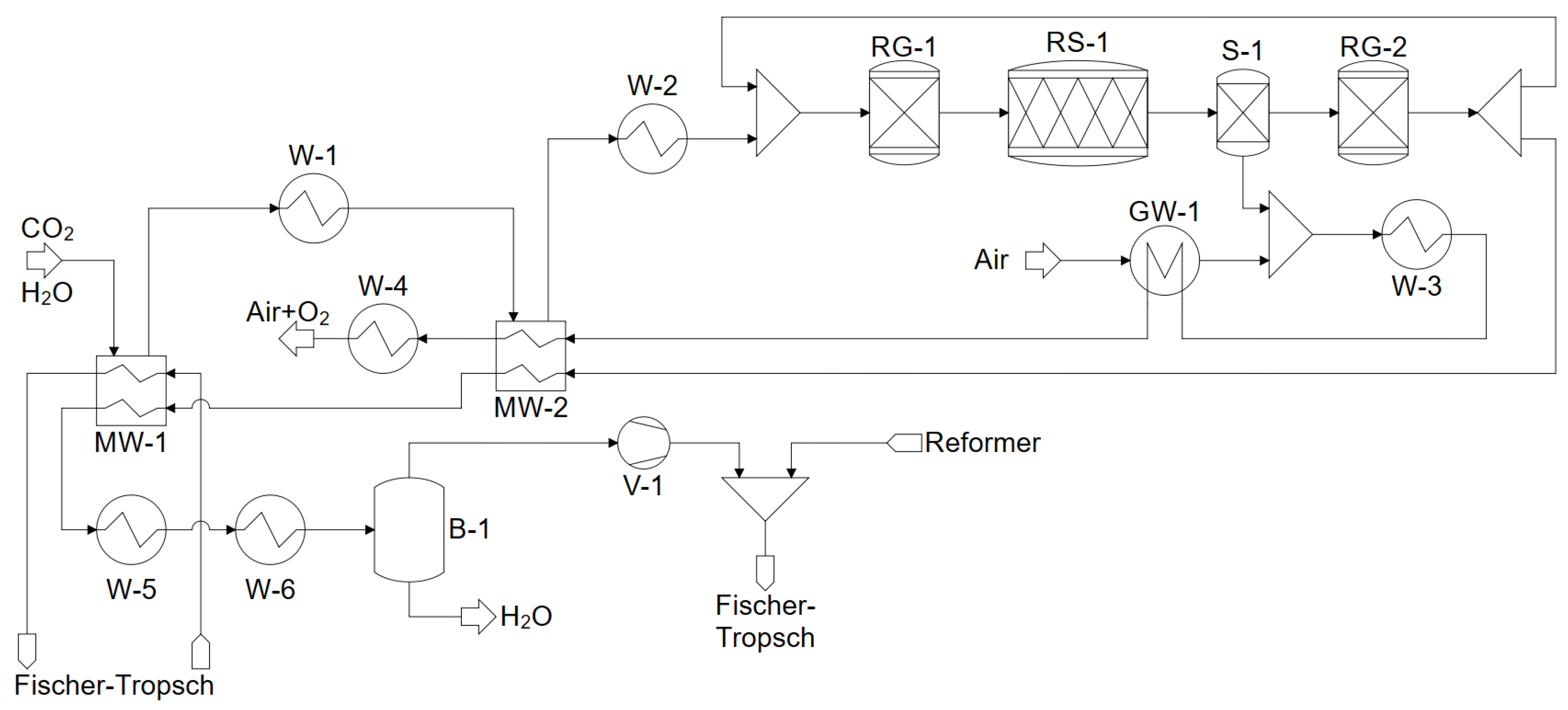
3.1. Electrolysis and Co-Electrolysis
3.2. Fischer–Tropsch Synthesis
- is the ratio of the speeds of the chain growth rate and chain growth termination rate
- ();
- is the hydrogen concentration in mol/m3;
- is the carbon monoxide concentration in mol/m3;
- is the exponential parameter for selectivity ();
- is the difference of activation energies for chain growth and chain growth termination ();
- is the ideal gas constant (); and
- is the reactor temperature in K.
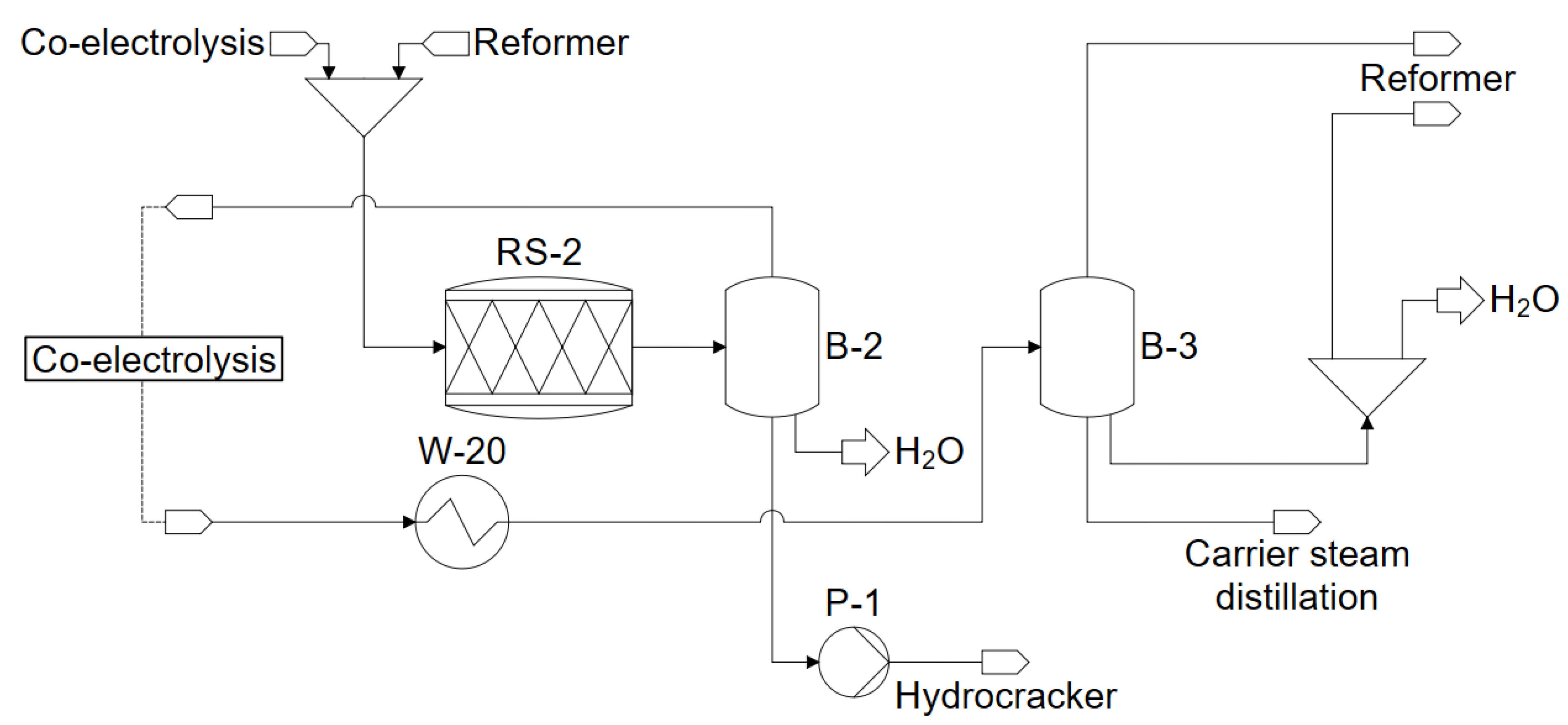
3.3. Hydrocrackers
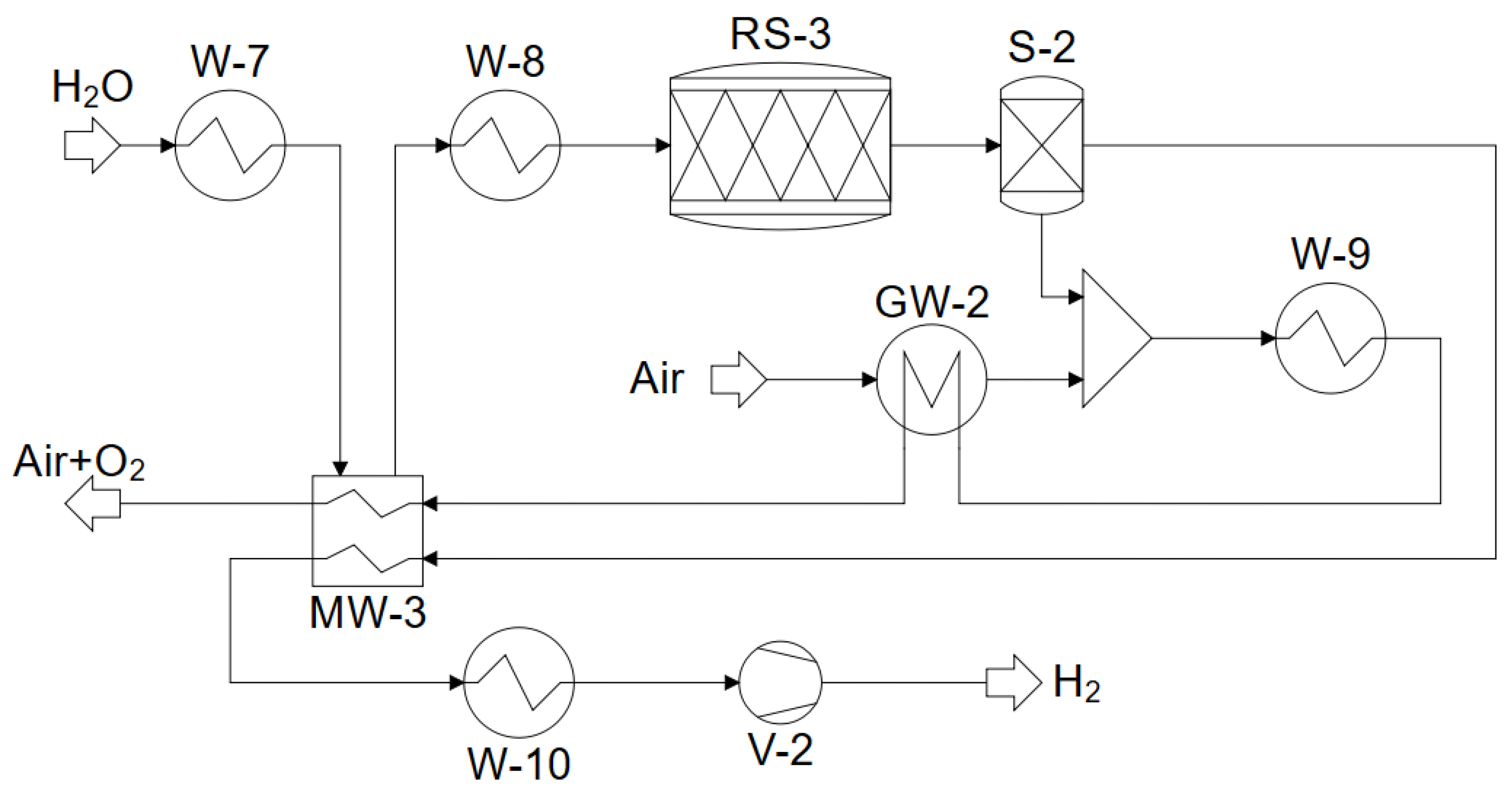
3.4. Reformers–Steam Reforming and Partial Oxidation
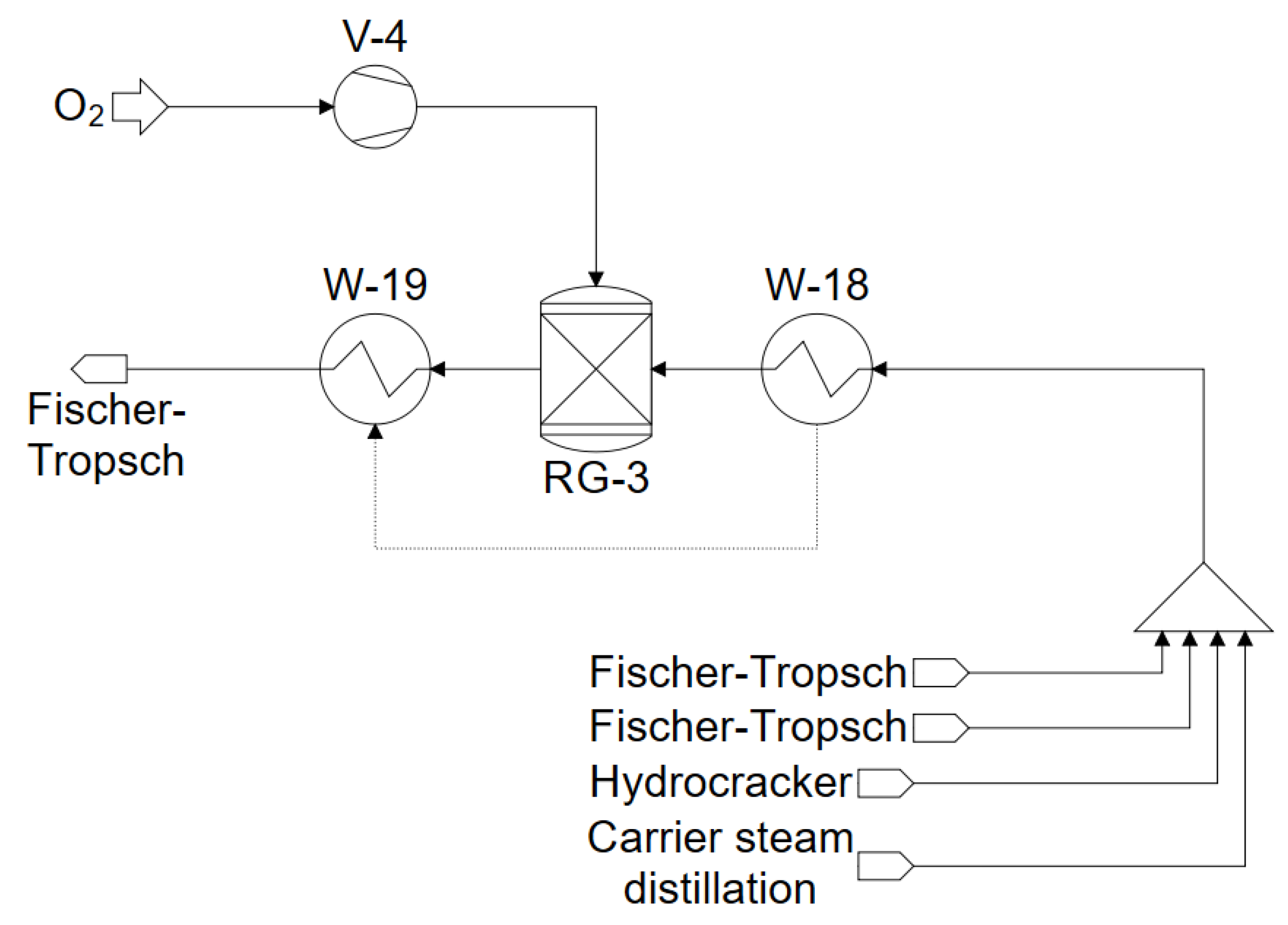
3.5. Carrier Steam Distillation
3.6. Technology Readiness Level
4. Modeling and Simulation in ASPEN PLUS
4.1. Material Property Data and Material Property Data Models
4.2. Co-Electrolysis and Water Electrolysis
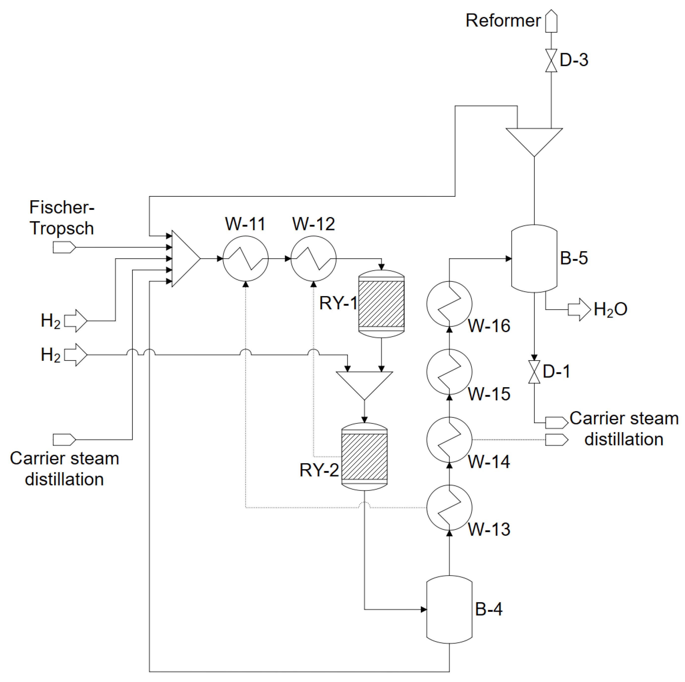
4.3. Fischer–Tropsch Synthesis and Product Separation
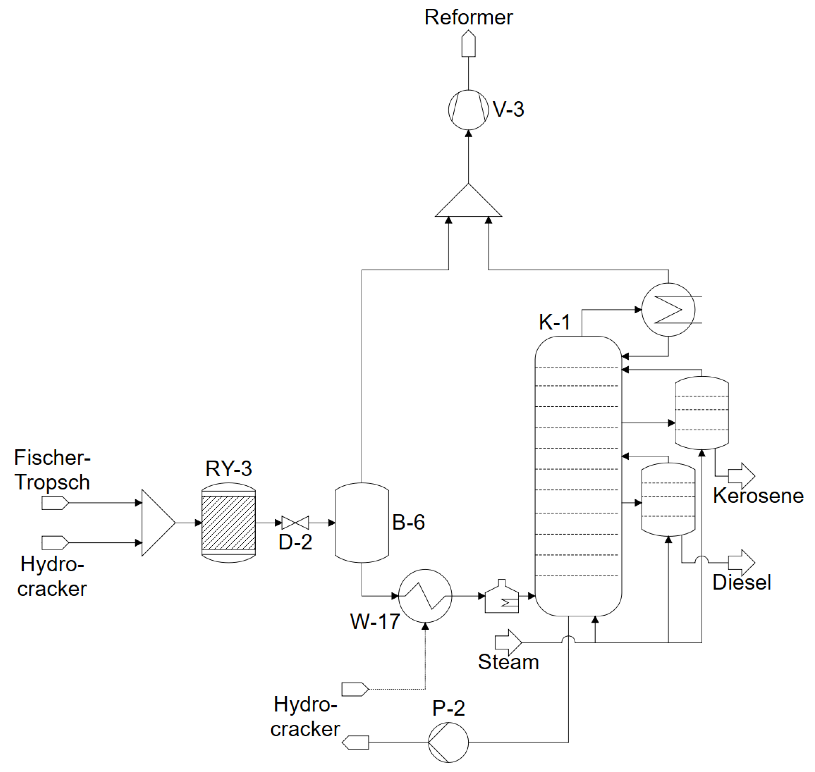
4.4. Hydrocracker
4.5. Carrier Steam Distillation
4.6. Reformer
5. Results from Process Analysis
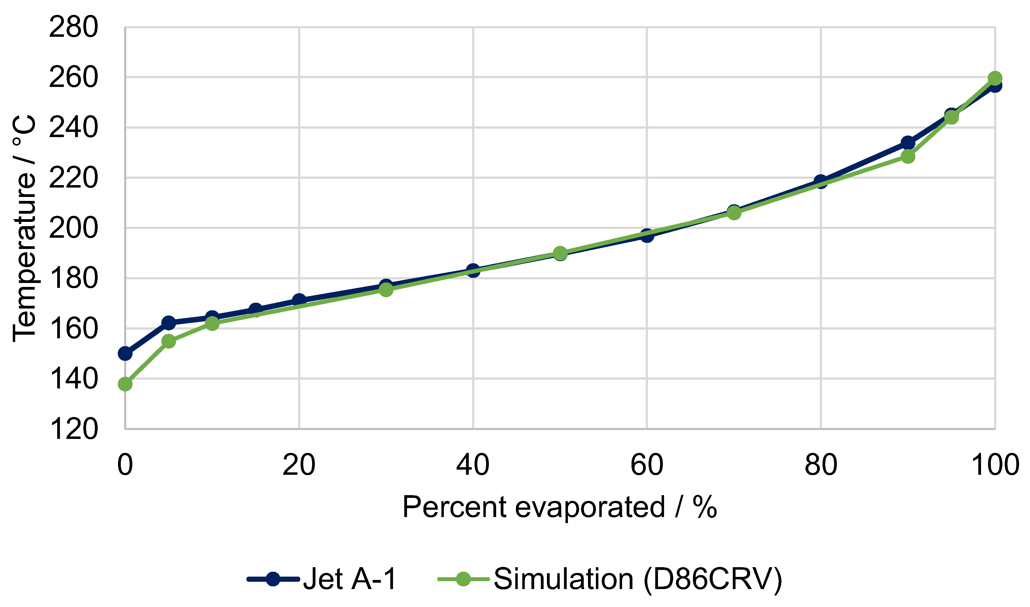
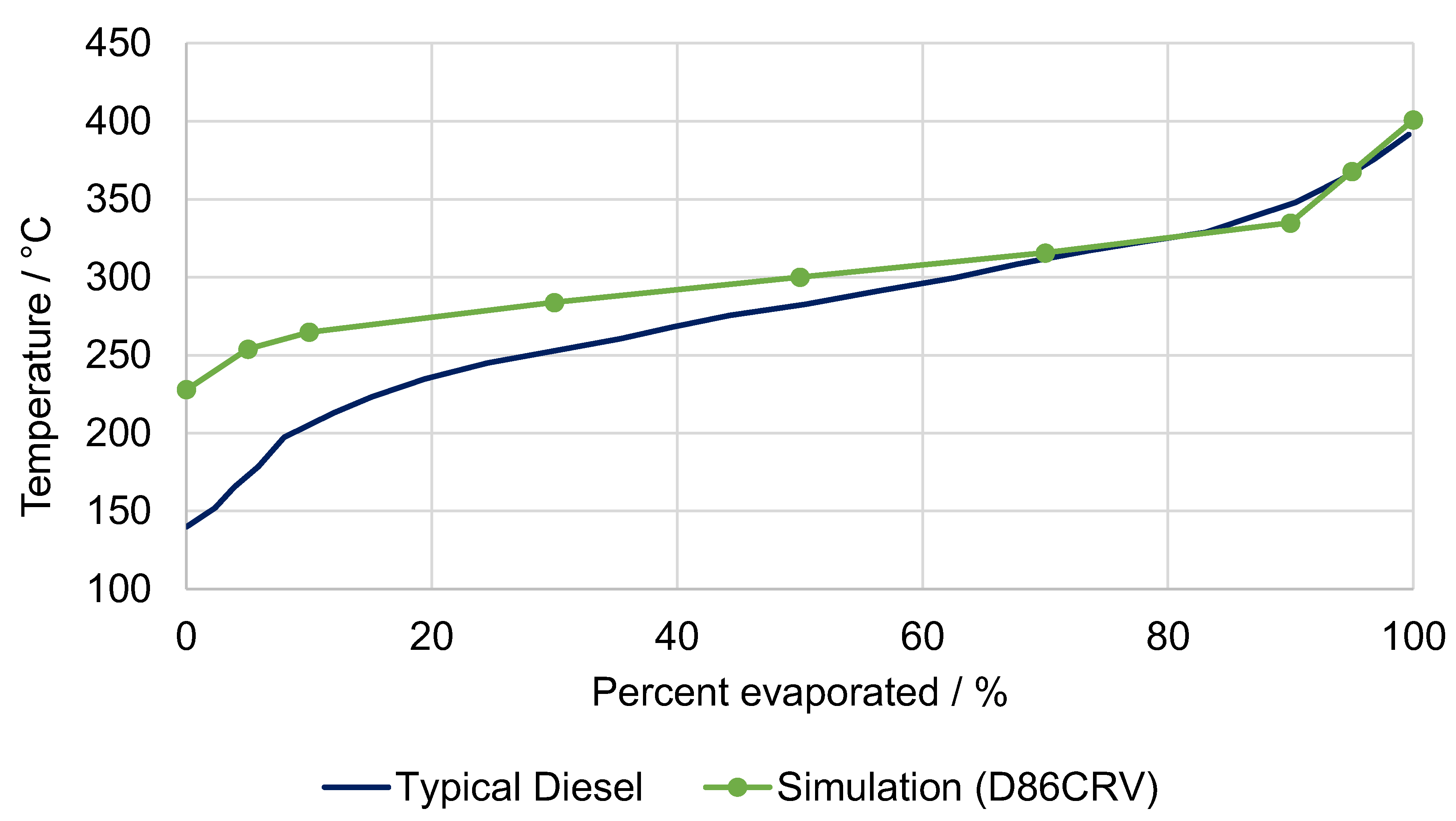
5.1. Fuel Property Analysis
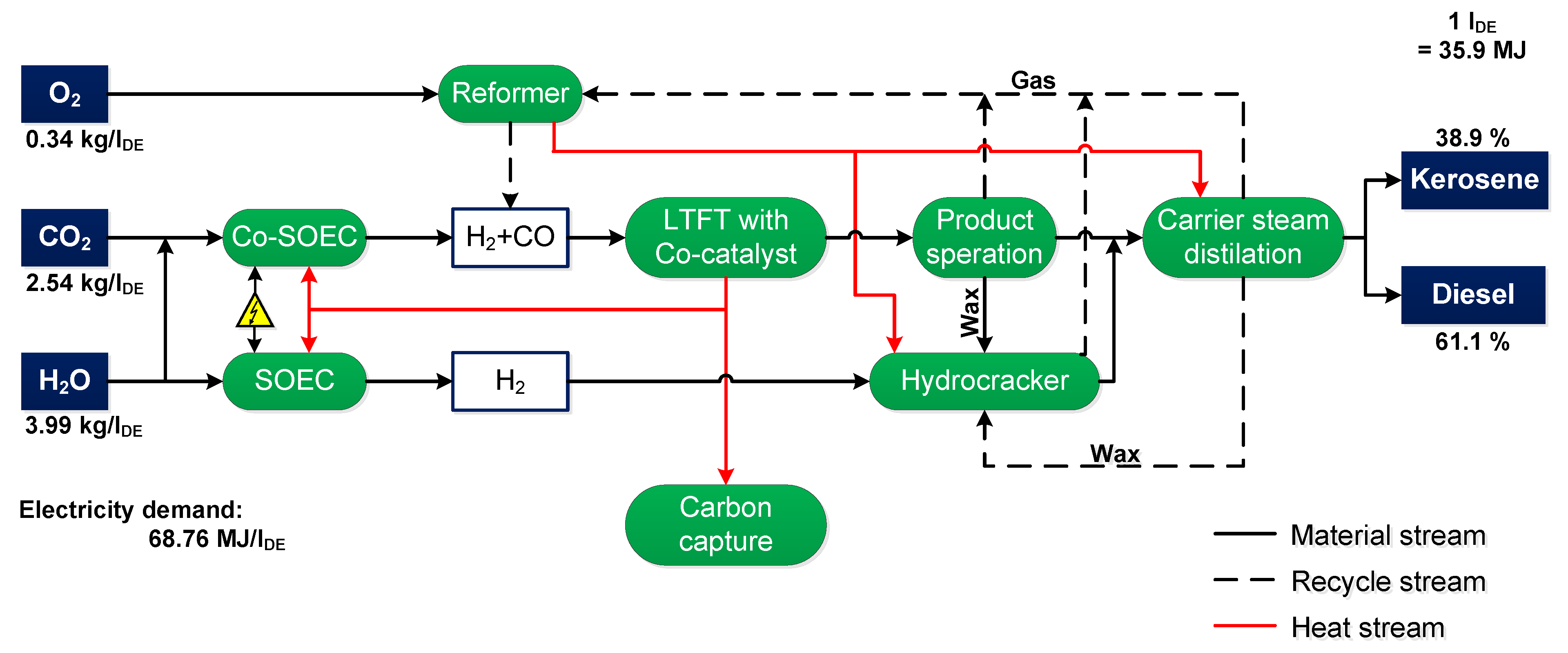
5.2. Balancing the Power-to-Fuel Process
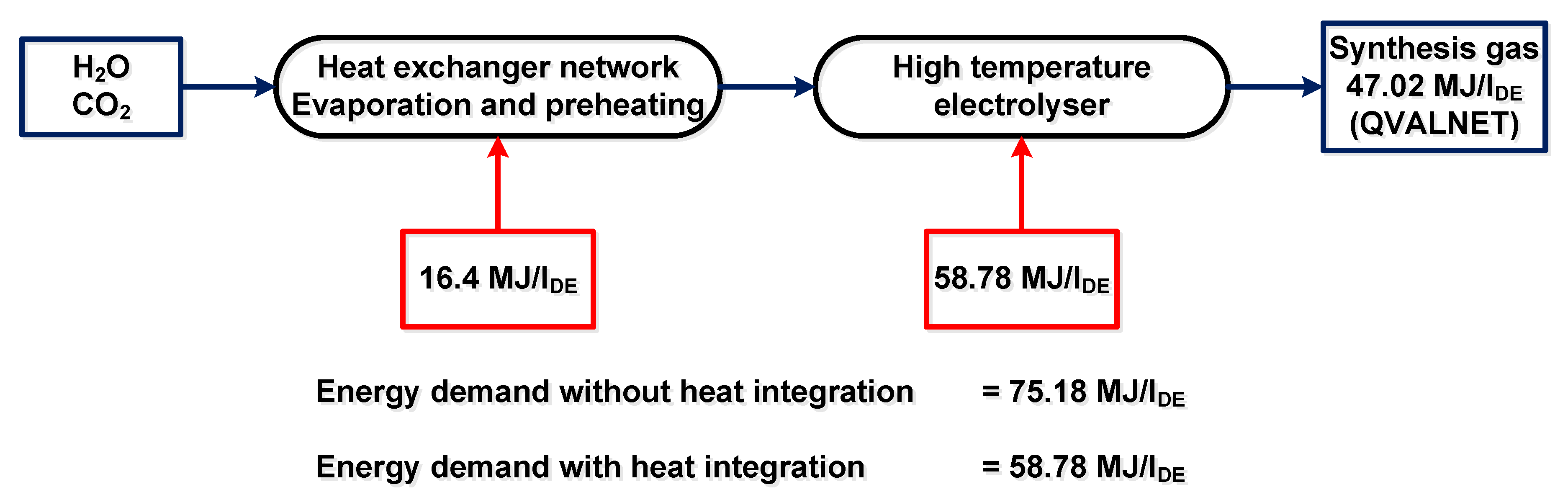
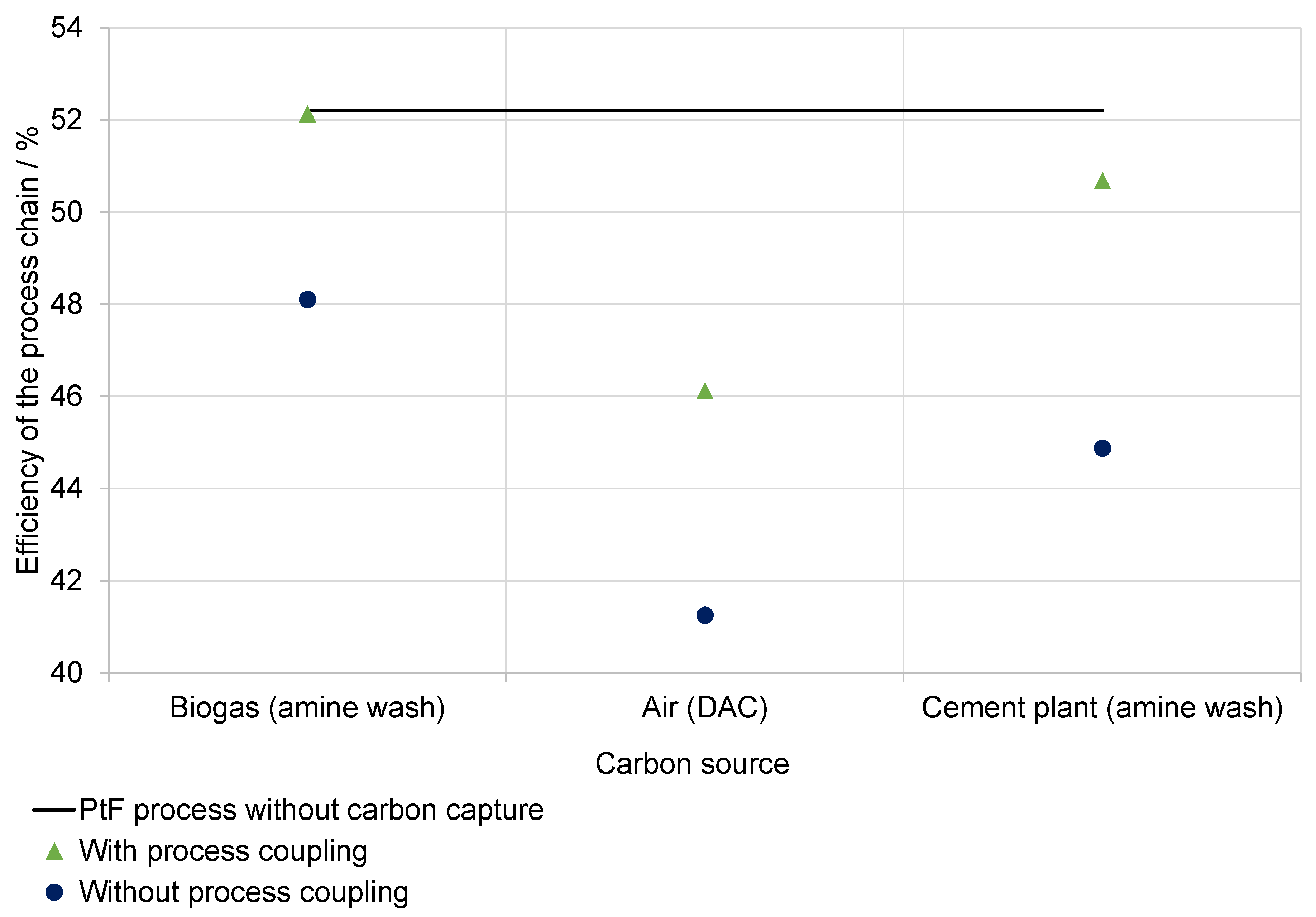
5.3. Heat Recuperation and CO2 Separation
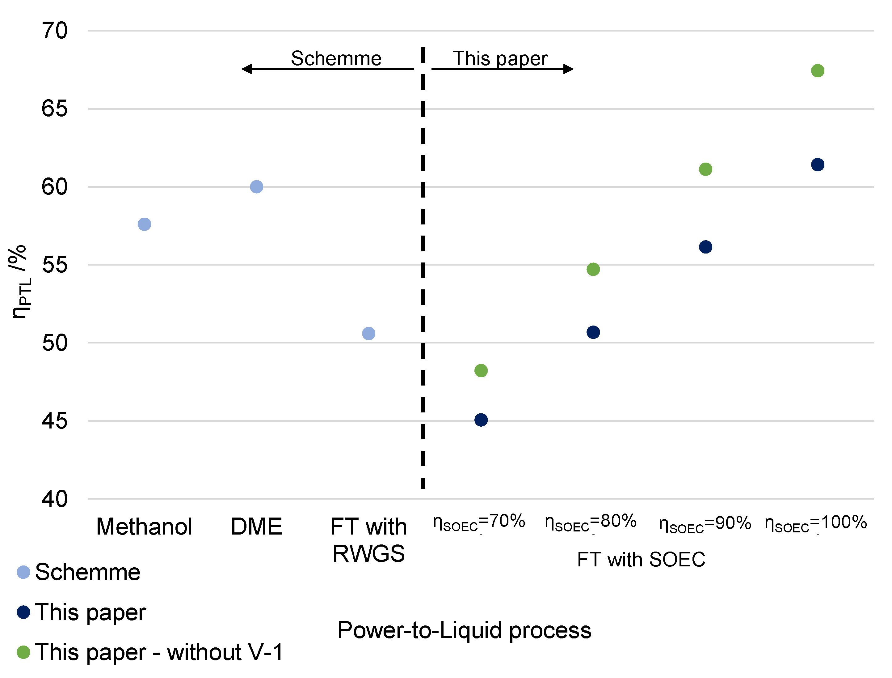
5.4. Comparison to a Related Analysis for E-Fuels Based on Low-Temperature Electrolysis
6. Techno-Economic Analysis
6.1. Investment Cost
6.2. Material and Personnel Costs
6.3. Product Cost
- Investment costs FCI = €949.9 million, see Table 4;
- Personnel costs Cp = €3.37 million, see Equation (23);
- Raw material costs CR = €63.6 million, see Table 6;
- Operating costs CB = €243.5 million, see Table 6;
- Depreciation period t = 12;
- Interest rate i = 0.05.
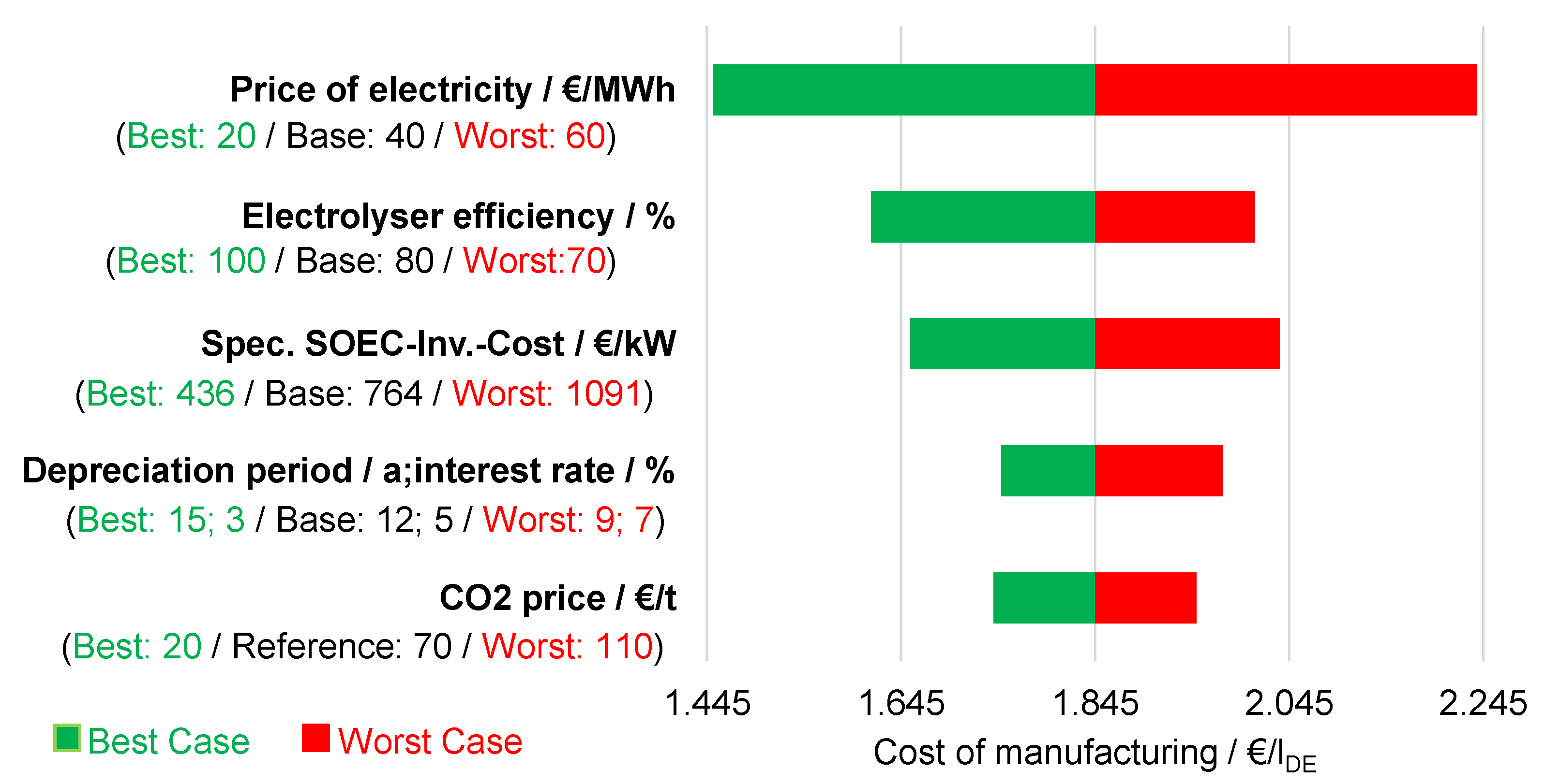
6.4. Sensitivity Analysis
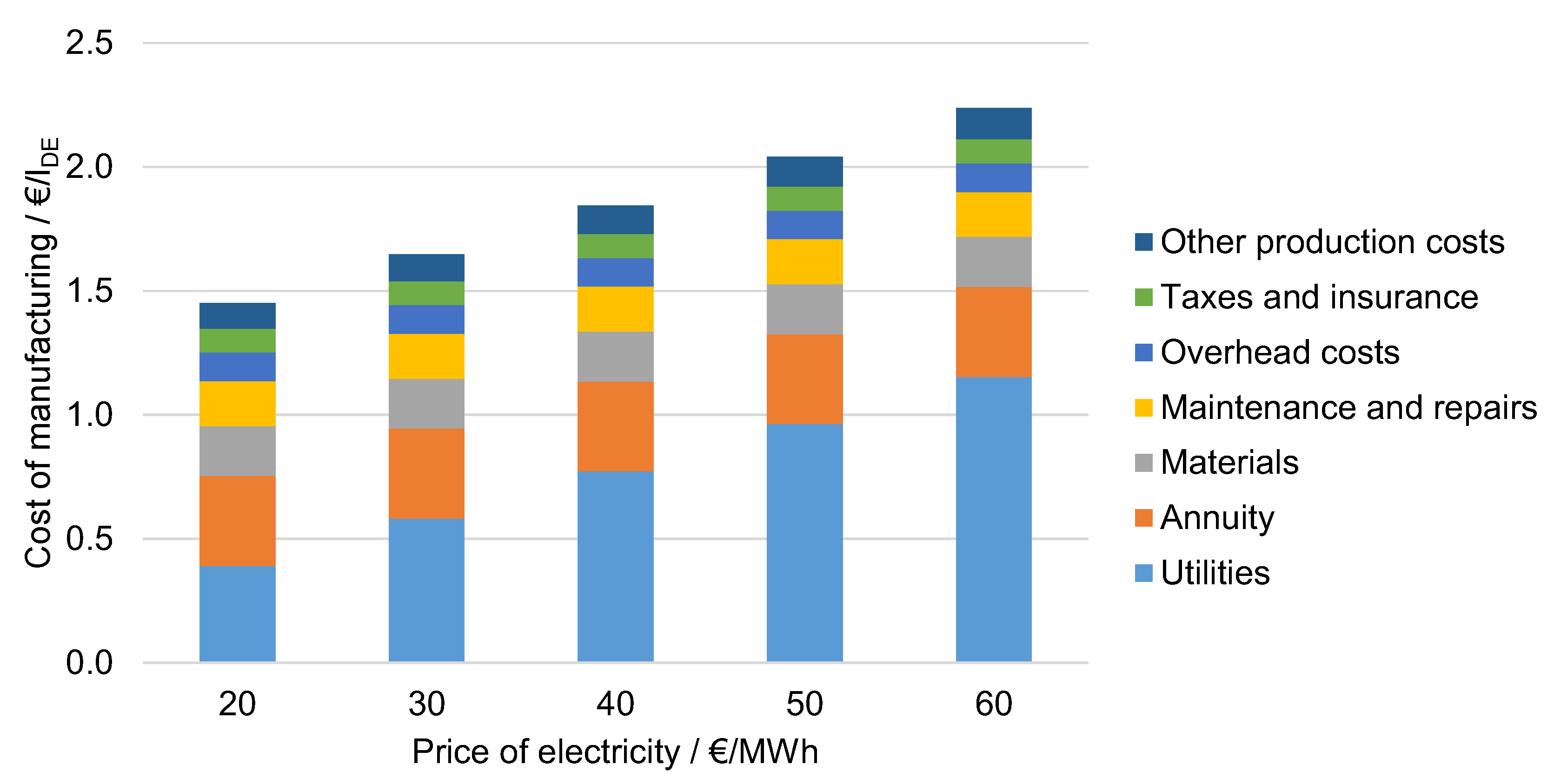
6.4.1. Influence of the Electricity Price
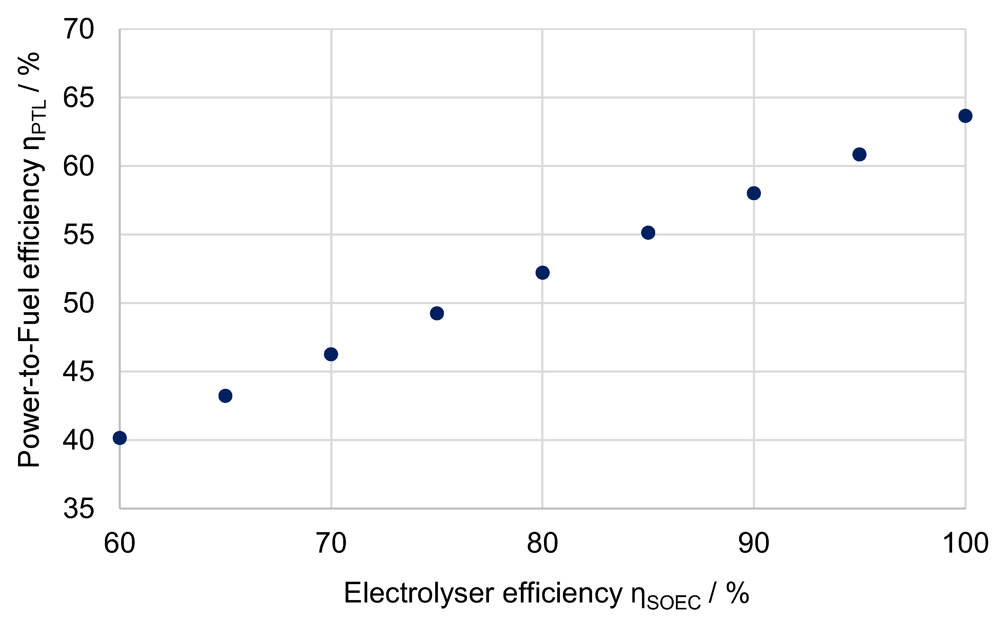
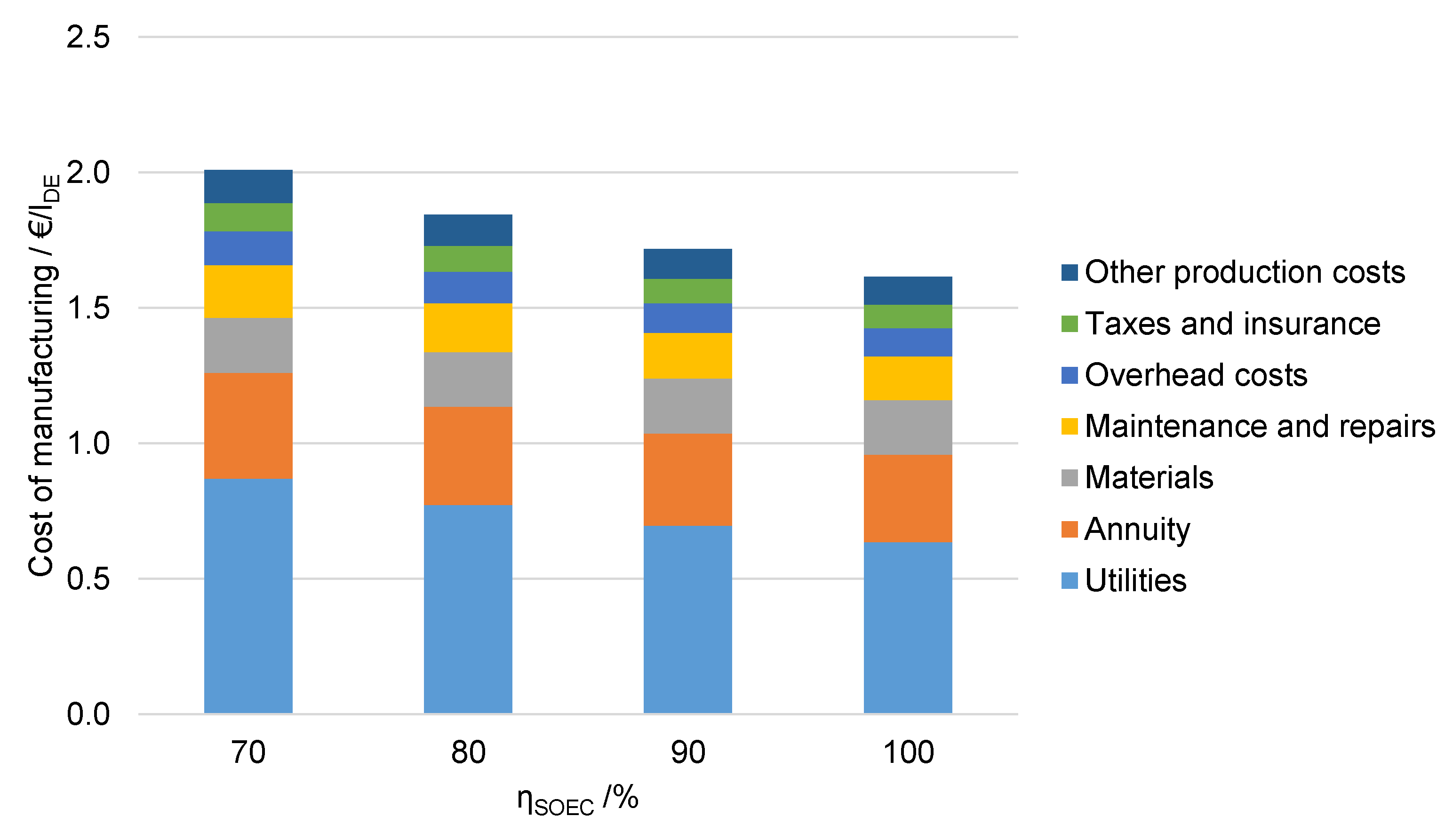
6.4.2. Influence of Electrolysis Efficiency
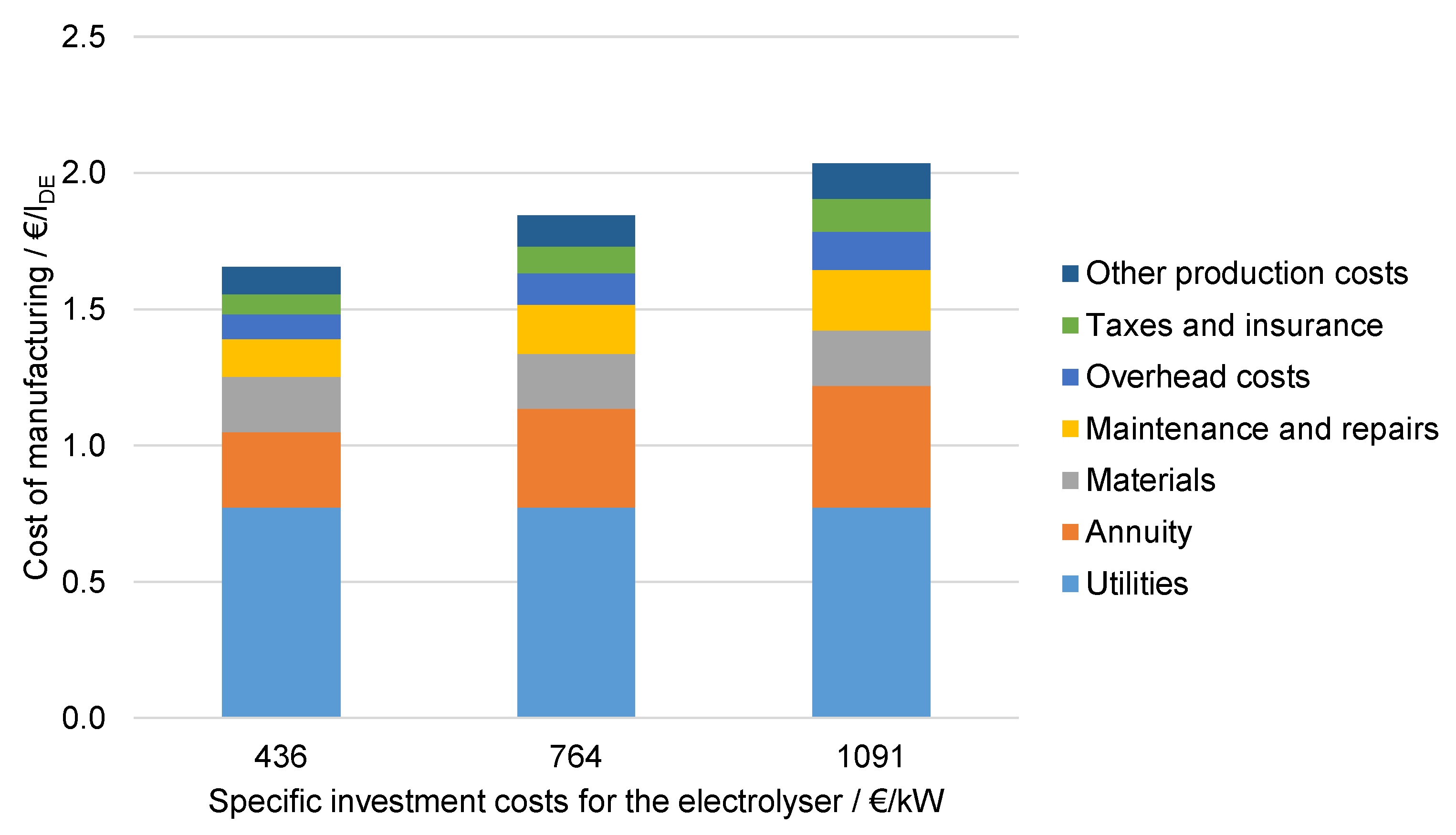
6.4.3. Influence of the Specific Investment Costs for Electrolysis
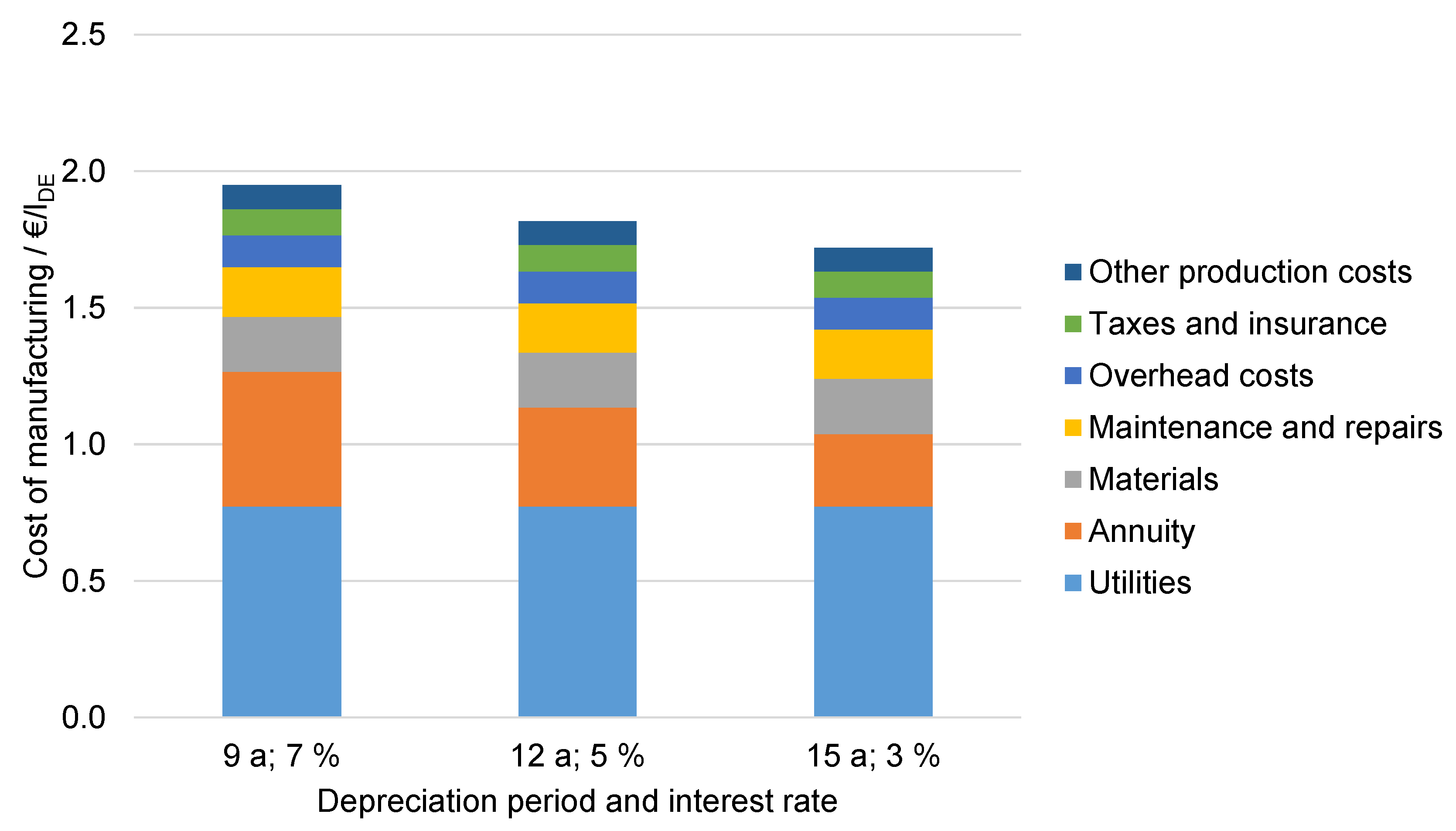
6.4.4. Influence of the Depreciation Period and Interest Rate
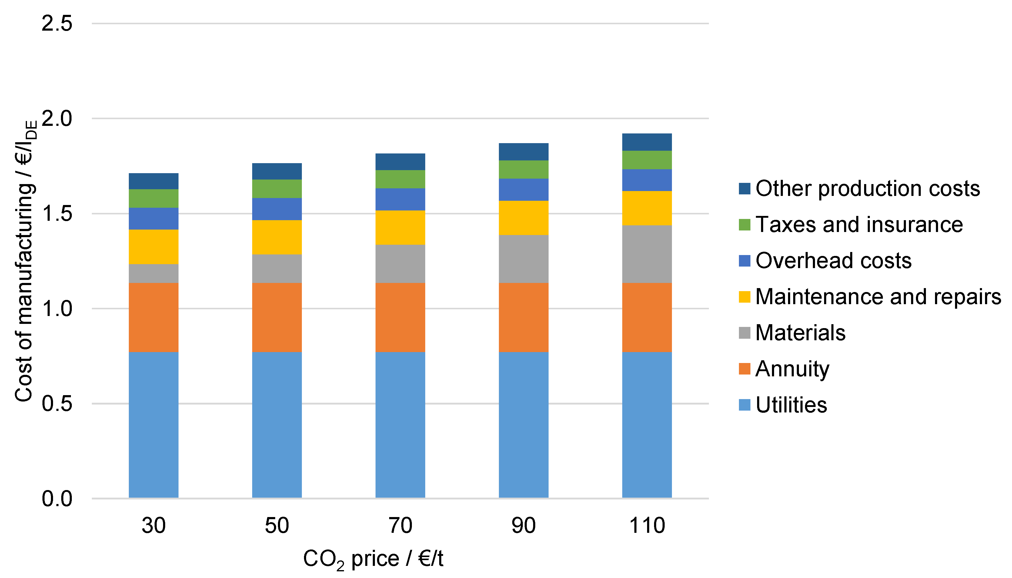
6.4.5. Influence of CO2 Costs
6.4.6. Influence of the Cost Factors in Comparison
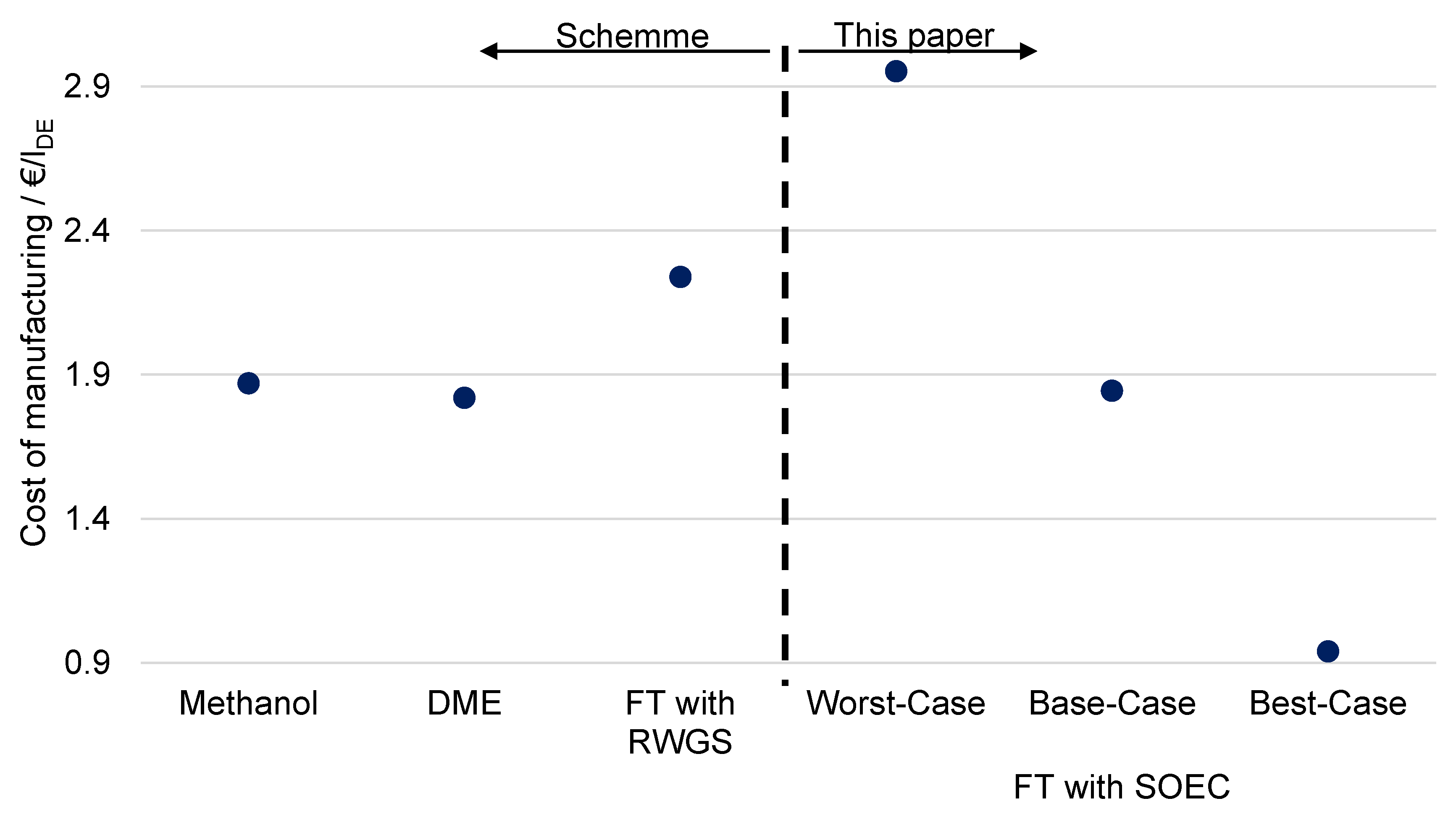
6.5. Comparison with Alternative Power-to-Liquid Processes
7. Conclusions
Author Contributions
Funding
Acknowledgments
Conflicts of Interest
Abbreviations
| SRK | Equation of State (EOS, cubic) Soave–Redlich–Kwong |
| RKS-BM | Soave–Redlich–Kwong EOS with Boston–Mathias Alpha-Function |
| BK10 | Braun K-10 |
| NRTL-RK | Non-Random-Two-Liquid, extended by EOS Redlich–Kwong for calculation of the gas phase |
Appendix A. Effect of Chain Growth Probability on the Product Distribution

Appendix B. Key Data from Process Simulations

| Input | Output | ||
|---|---|---|---|
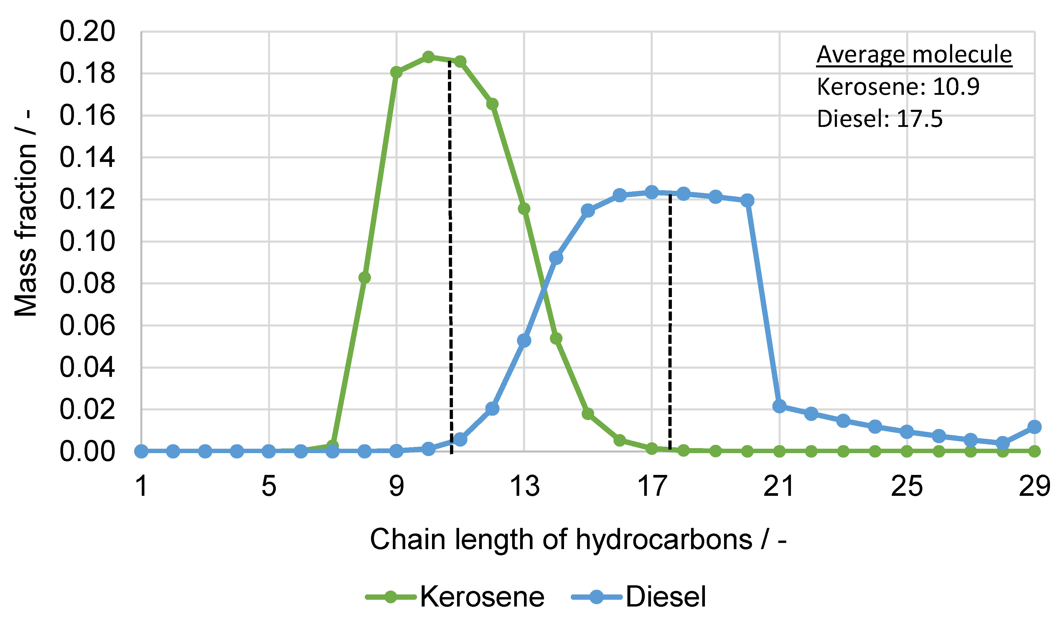
| Carbon dioxide | 2.54 kg | Synthetic fuel | 1 lDE |
| Water | 3.99 kg | Share kerosene | 38.9% |
| Oxygen | 0.34 kg | Share diesel | 61.9% |
| Water | 2.89 kg | ||
| Resources | Temperature Range | Specific Heating-/Cooling-Power |
|---|---|---|
| Low-pressure saturated steam | 124–125 °C | 2193 kJ/kg |
| Medium-pressure saturated steam | 174–175 °C | 2036 kJ/kg |
| Cooling water | 20–25 °C | 21 kJ/kg |
| Cooling air | 30–35 °C | 5 kJ/kg |
| Electricity | - | - |
| Resources | Quantity [kg/lDE] | Energy [MJ/lDE] |
|---|---|---|
| Low-pressure saturated steam | ||
| Produced | −0.235 | −0.515 |
| Demand | 0.196 | 0.429 |
| Sum | −0.039 | −0.086 |
| Medium-pressure saturated steam | ||
| Produced | −6.059 | −12.339 |
| Demand | 1.546 | 3.148 |
| Sum | −4.513 | −9.191 |
| Cooling water | ||
| Demand | 84.370 | 1.764 |
| Cooling air | ||
| Demand | 1086.192 | 5.431 |
| Electricity (w/o electrolysis) | ||
| Demand | - | 6.890 |
| FT Reactor | Hydrocracker | Reformer | |
|---|---|---|---|
| Educt-/product rate | 350,322 Nm3/h | 1191 t/d | 159,483 Nm3/h |
| -value | 228,029 Nm3/h | 6256 t/d | 9,438,667 Nm3/h |
| Number of reactors | 2 | 1 | 1 |
References
- BMU. Klimaschutz in Zahlen-Fakten, Trends und Impulse deutscher Klimapolitik; Bundesministerium für Umwelt, Naturschutz und nuklear Sicherheit (BMU): Berlin, Germany, 2019. [Google Scholar]
- Ausfelder, F.; Wagemann, K. Power-to-Fuels: E-Fuels as an Important Option for a Climate-Friendly Mobility of the Future. Chem. Ing. Tech. 2020, 92, 21–30. [Google Scholar] [CrossRef]
- Sterner, M.; Stadler, I. Energiespeicher-Bedarf, Technologien, Integration, 2nd ed.; Springer: Berlin/Heidelberg, Germany, 2017. [Google Scholar]
- Kramer, U. Defossilierung des Transportsektors Optionen und Vorraussetzungen in Deutschland; FVV Prime Movers. Technologies: Frankfurt am Main, Germany, 2018. [Google Scholar]
- Marlin, D.S.; Sarron, E.; Sigurbjornsson, O. Process Advantages of Direct CO2 to Methanol Synthesis. Front. Chem. 2018, 6, 446. [Google Scholar] [CrossRef] [PubMed]
- Dieterich, V.; Buttler, A.; Hanel, A.; Spliethoff, H.; Fendt, S. Power-to-liquid via synthesis of methanol, DME or Fischer–Tropsch-fuels: A review. Energy Environ. Sci. 2020, 13, 3207–3252. [Google Scholar] [CrossRef]
- Energiedaten: Gesamtausgabe. Available online: https://www.bmwi.de/Redaktion/DE/Artikel/Energie/energiedaten-gesamtausgabe.html (accessed on 31 October 2020).
- Schmidt, P.; Weindorf, W.; Roth, A.; Batteiger, V.; Riegel, F. Power-to-Liquids Potentials and Perspectives for the Future Supply of Renewable Aviation Fuel; Umweltbundesamt, Ed.; German Environment Agency: Dessau-Roßlau, Germany, 2016. [Google Scholar]
- De Klerk, A. Fischer-Tropsch Refining; Wiley-VCH Verlag & Co. KGaA: Weinheim, Germany, 2011. [Google Scholar]
- Schemme, S.; Samsun, R.C.; Peters, R.; Stolten, D. Power-to-fuel as a key to sustainable transport systems–An analysis of diesel fuels produced from CO2 and renewable electricity. Fuel 2017, 205, 198–221. [Google Scholar] [CrossRef]
- Verdegaal, W.M.; Becker, S.; Olshausen, C.V. Power-to-Liquids: Synthetisches Rohöl aus CO2, Wasser und Sonne. Chem. Ing. Tech. 2015, 87, 340–346. [Google Scholar] [CrossRef]
- GmbH, S. Blue Crude: Sunfire Produziert Nachhaltigen Erdölersatz. Available online: https://www.sunfire.de/de/unternehmen/news/detail/blue-crude-sunfire-produziert-nachhaltigen-erdoelersatz (accessed on 20 October 2020).
- Bazzanella, A.; Krämer, D. (Eds.) Technologies for Sustainability and Climate Protection-Chemical Processes and Use of CO2; DECHEMA Gesellschaft für Chemische Technik und Biotechnologie e.V.: Frankfurt, Germany, 2017. [Google Scholar]
- Vázquez, F.V.; Koponen, J.; Ruuskanen, V.; Bajamundi, C.; Kosonen, A.; Simell, P.; Ahola, J.; Frilund, C.; Elfving, J.; Reinikainen, M.; et al. Power-to-X technology using renewable electricity and carbon dioxide from ambient air: SOLETAIR proof-of-concept and improved process concept. J. CO2 Util. 2018, 28, 235–246. [Google Scholar] [CrossRef]
- SOLETAIR-Technical Specifications. Available online: https://soletair.fi/technical-specifications/ (accessed on 20 October 2020).
- Durchbruch Für Power-to-X. Available online: https://www.kopernikus-projekte.de/aktuelles?backRef=30&news=Durchbruch_fuer_Power_to_X (accessed on 20 October 2020).
- Durchbruch Für Power-to-X: Sunfire Nimmt Erste Co-Elektrolyse in Betrieb und Startet die Skalierung. Available online: https://www.sunfire.de/de/unternehmen/news/detail/durchbruch-fuer-power-to-x-sunfire-nimmt-erste-co-elektrolyse-in-betrieb-und-startet-die-skalierung (accessed on 20 October 2020).
- Norsk e-Fuel. Available online: https://www.norsk-e-fuel.com/en/ (accessed on 8 September 2020).
- Translated: Two Companies Want to Make Synthetic Fuel on Herøya: Ex-Partner Becomes a Competitor and Settles on the Neighboring Plot. Available online: https://www.tu.no/artikler/to-bedrifter-vil-lage-syntetisk-drivstoff-pa-heroya-eks-partner-blir-konkurrent-og-slar-seg-ned-pa-nabotomta/493866?key=zbh08EHG (accessed on 8 September 2020).
- Trotz Wasserstoffstrategie: Große Power-to-X-Anlage von Norsk e-Fuel Entsteht in Norwegen. Available online: https://www.cleanthinking.de/wasserstoffstrategie-powertox-norsk-e-fuel-norwegen/ (accessed on 8 September 2020).
- The Hague Airport Initiates Study for the Production of Renewable Jet Fuel from Air. Available online: https://www.sunfire.de/de/unternehmen/news/detail/rotterdam-the-hague-airport-initiates-study-for-the-production-of-renewable-jet-fuel-from-air (accessed on 20 October 2020).
- Schiphol and Sustainable Kerosene. Available online: https://news.schiphol.com/schiphol-and-sustainable-kerosene/ (accessed on 8 September 2020).
- Zenid–Sustainable Aviation Fuel from Air. Available online: https://climeworks.com/news/christoph-gebald-co-ceo-and-co-founder-of-climeworks (accessed on 8 September 2020).
- Zenid | Jet Fuel from Air. Available online: https://zenidfuel.com/ (accessed on 8 September 2020).
- Homepage-Synkero. Available online: https://synkero.com/ (accessed on 8 September 2020).
- Carmo, M.; Fritz, D.L.; Mergel, J.; Stolten, D. A comprehensive review on PEM water electrolysis. Int. J. Hydrogen Energy 2013, 38, 4901–4934. [Google Scholar] [CrossRef]
- Andika, R.; Nandiyanto, A.B.D.; Putra, Z.A.; Bilad, M.R.; Kim, Y.; Yun, C.M.; Lee, M. Co-electrolysis for power-to-methanol applications. Renew. Sustain. Energy Rev. 2018, 95, 227–241. [Google Scholar] [CrossRef]
- Zheng, Y.; Wang, J.; Yu, B.; Zhang, W.; Chen, J.; Qiao, J.; Zhang, J. A review of high temperature co-electrolysis of H2O and CO2 to produce sustainable fuels using solid oxide electrolysis cells (SOECs): Advanced materials and technology. Chem. Soc. Rev. 2017, 46, 1427–1463. [Google Scholar] [CrossRef]
- Buttler, A.; Spliethoff, H. Current status of water electrolysis for energy storage, grid balancing and sector coupling via power-to-gas and power-to-liquids: A review. Renew. Sustain. Energy Rev. 2018, 82, 2440–2454. [Google Scholar] [CrossRef]
- Dueñas, D.M.A.; Riedel, M.; Riegraf, M.; Costa, R.; Friedrich, K.A. High Temperature Co-electrolysis for Power-to-X. Chem. Ing. Tech. 2020, 92, 45–52. [Google Scholar] [CrossRef] [Green Version]
- Cinti, G.; Baldinelli, A.; Di Michele, A.; Desideri, U. Integration of Solid Oxide Electrolyzer and Fischer-Tropsch: A sustainable pathway for synthetic fuel. Appl. Energy 2016, 162, 308–320. [Google Scholar] [CrossRef]
- Frank, M.H. Reversible Wasserstoffbetriebene Festoxidzellensysteme; Forschungszentrum Jülich GmbH Zentralbibliothek: Jülich, Germany, 2019. [Google Scholar]
- Marchese, M.; Giglio, E.; Santarelli, M.; Lanzini, A. Energy performance of Power-to-Liquid applications integrating biogas upgrading, reverse water gas shift, solid oxide electrolysis and Fischer-Tropsch technologies. Energy Convers. Manag. X 2020, 6, 100041. [Google Scholar] [CrossRef]
- Peters, R.; Decker, M.; Eggemann, L.; Schemme, S.; Schorn, F.; Breuer, J.L.; Weiske, S.; Pasel, J.; Samsun, R.C.; Stolten, D. Thermodynamic and ecological preselection of synthetic fuel intermediates from biogas at farm sites. Energy Sustain. Soc. 2020, 10, 4. [Google Scholar] [CrossRef]
- Trippe, F. Techno-Ökonomische Bewertung Alternativer Verfahrenskonfigurationen Zur Herstellung Biomass-to-Liquid (BtL) Kraftstoffen und Chemikalien; KIT: Karlsruhe, Germany, 2013. [Google Scholar]
- de Klerk, A. Fischer–Tropsch fuels refinery design. Energy Environ. Sci. 2011, 4, 1177–1205. [Google Scholar] [CrossRef]
- Holladay, J.; Albrecht, K.; Hallen, R. Renewable routes to jet fuel. Curr. Opin. Biotechnol. 2014, 26, 50–55. [Google Scholar]
- Vervloet, D.; Kapteijn, F.; Nijenhuis, J.; van Ommen, J.R. Fischer–Tropsch reaction–diffusion in a cobalt catalyst particle: Aspects of activity and selectivity for a variable chain growth probability. Catal. Sci. Technol. 2012, 2, 1221–1233. [Google Scholar] [CrossRef]
- Hsu, C.S.; Robinson, P.R. (Eds.) Practical Advances in Petroleum Processing; Springer: New York, NY, USA, 2006; Volume 1. [Google Scholar]
- Speight, J.G. Heavy and Extra-Heavy Oil Upgrading Technologies; Gulf Professional Publishing: Houston, TX, USA; Elsevier Inc.: Amsterdam, The Netherlands, 2013. [Google Scholar] [CrossRef]
- Bouchy, C.; Hastoy, G.; Guillon, E.; Martens, J.A. Fischer-Tropsch Waxes UpgradingviaHydrocracking and Selective Hydroisomerization. Oil Gas Sci. Technol. 2009, 64, 91–112. [Google Scholar] [CrossRef] [Green Version]
- Calemma, V.; Gambaro, C.; Parker, W.O.; Carbone, R.; Giardino, R.; Scorletti, P. Middle distillates from hydrocracking of FT waxes: Composition, characteristics and emission properties. Catal. Today 2010, 149, 40–46. [Google Scholar] [CrossRef]
- Wegener, N. Prozessmodellierung und Bewertung Synthetischer Kraftstoffe auf Basis von Wasserstoff und Kohlenstoffdioxid. Master’s Thesis, University of Bochum, Bochum, Germany, 2020. [Google Scholar]
- Lawson, K.H.; Jothimurugesan, K.; Espinoza, R.L. Catalyst for Hydroprocessing of Fischer-Tropsch Products. U.S. Patent 10/866,884, 15 December 2005. [Google Scholar]
- Meyers, R.A. Handbook of Petroleum Refining Processes, 3rd ed.; McGraw-Hill: New York, NY, USA, 2004. [Google Scholar]
- Pors, Z. Eduktvorbereitung und Gemischbildung in Reaktionsapparaten zur Autothermen Reformierung von Dieselähnlichen Kraftstoffen; Forschungszentrum Jülich GmbH Zentralbibliothek: Jülich, Germany, 2006. [Google Scholar]
- Rostrup-Nielsen, J.R. Syngas in perspective. Catal. Today 2002, 71, 243–247. [Google Scholar] [CrossRef]
- Luyben, W.L. Distillation Design and Control Using Aspen(TM) Simulation, 2nd ed.; John Wiley & Sons: Hoboken, NJ, USA, 2013. [Google Scholar]
- Tzinis, I. Technology Readiness Level. Available online: https://www.nasa.gov/directorates/heo/scan/engineering/technology/technology_readiness_level (accessed on 22 February 2022).
- Héder, M. From NASA to EU: The evolution of the TRL scale in Public Sector Innovation. Innov. J. 2017, 22, 1. [Google Scholar]
- De Rose, A.; Buna, M.; Strazza, C.; Olivieri, N.; Stevens, T.; Peeters, L. Technology Readiness Level: Guidance Principles for Renewable Energy Technologies; European Comission: Brussels, Belgium, 2017. [Google Scholar]
- de Klerk, A. Can Fischer−Tropsch Syncrude Be Refined to On-Specification Diesel Fuel? Energy Fuels 2009, 23, 4593–4604. [Google Scholar] [CrossRef]
- Dry, M.E. High quality diesel via the Fischer-Tropsch process—A review. J. Chem. Technol. Biotechnol. 2002, 77, 43–50. [Google Scholar] [CrossRef]
- Schemme, S. Techno-Ökonomische Bewertung von Verfahren zur Herstellung von Kraftstoffen aus H2 und CO2; Forschungszentrum Jülich GmbH Zentralbibliothek: Jülich, Germany, 2020. [Google Scholar]
- Carlson, E.C. Don’t Gamble With Physical Properties For Simulations. Chem. Eng. Prog. 1996, 92, 35–46. [Google Scholar]
- Auburn University. Design of a Process for the Production if Fuels and/or Chemicals from Hydrocarbon Feestocks; Department of Chemical Engineering, Auburn University: Auburn, AL, USA, 2013. [Google Scholar]
- Sun, X.; Chen, M.; Jensen, S.H.; Ebbesen, S.D.; Graves, C.; Mogensen, M. Thermodynamic analysis of synthetic hydrocarbon fuel production in pressurized solid oxide electrolysis cells. Int. J. Hydrogen Energy 2012, 37, 17101–17110. [Google Scholar] [CrossRef]
- Cinti, G.; Discepoli, G.; Bidini, G.; Lanzini, A.; Santarelli, M. Co-electrolysis of water and CO2 in a solid oxide electrolyzer (SOE) stack. Int. J. Energy Res. 2016, 40, 207–215. [Google Scholar] [CrossRef]
- Becker, W.L.; Braun, R.J.; Penev, M.; Melaina, M. Production of Fischer–Tropsch liquid fuels from high temperature solid oxide co-electrolysis units. Energy 2012, 47, 99–115. [Google Scholar] [CrossRef]
- Bacha, J.; Freel, J.; Gibbs, A.; Gibbs, L.; Hemighaus, G.; Hoekman, K.; Horn, J.; Gibbs, A.; Ingham, M.; Jossens, L.; et al. Diesel Fuels Technical Review; Chevron: San Ramon, CA, USA, 2017. [Google Scholar]
- Edwards, T. Reference Jet Fuels for Combustion Testing; Air Force Research Laboratory: Dayton, OH, USA, 2017. [Google Scholar]
- Cookson, D.J.; Lloyd, C.P.; Smith, B.E. Investigation of the Chemical Basis of Kerosene (Jet Fuel) Specification Properties. Energy Fuels 1987, 1, 438–447. [Google Scholar] [CrossRef]
- Martin, W.; Sandra, U.; Peter, M.; Friedrich, S.; Fabio, G. Energietechnologien der Zukunft-Erzeugung, Speicherung, Effizienz und Netze; Springer Vieweg: Wiesbaden, Germany, 2015. [Google Scholar] [CrossRef] [Green Version]
- Peters, R.; Deja, R.; Blum, L.; Nguyen, V.N.; Fang, Q.; Stolten, D. Influence of operating parameters on overall system efficiencies using solid oxide electrolysis technology. Int. J. Hydrogen Energy 2015, 40, 7103–7113. [Google Scholar] [CrossRef]
- Kuramochi, T.; Ramírez, A.; Turkenburg, W.; Faaij, A. Comparative assessment of CO2 capture technologies for carbon-intensive industrial processes. Prog. Energy Combust. Sci. 2012, 38, 87–112. [Google Scholar] [CrossRef]
- Peter, V.; Juri, H.; Alexander, S.; Ole, Z. Verfahren der CO2-Abtrennung aus Faulgasen und Umgebungsluft innerhalb des Forschungsprojekts TF_Energiewende; Wuppertal Institut für Klima, Umwelt, Energie gGmbH: Wuppertal, Germany, 2018. [Google Scholar]
- Lettenmeier, P. Wirkungsgrad-Elektrolyse-Whitepaper; Siemens, Corporate Technology, Strategy & Business Development: Erlangen, Germany, 2019. [Google Scholar]
- Metz, B.; Davidson, O.; de Coninck, H.; Loos, M.; Meyer, L. (Eds.) Carbon Dioxide Capture and Storage; Cambridge University Press: New York, NY, USA, 2005. [Google Scholar]
- Peters, R.; Baltruweit, M.; Grube, T.; Samsun, R.C.; Stolten, D. A techno economic analysis of the power to gas route. J. CO2 Util. 2019, 34, 616–634. [Google Scholar] [CrossRef]
- Schemme, S.; Breuer, J.L.; Köller, M.; Meschede, S.; Walman, F.; Samsun, R.C.; Peters, R.; Stolten, D. H2-based synthetic fuels: A techno-economic comparison of alcohol, ether and hydrocarbon production. Int. J. Hydrogen Energy 2020, 45, 5395–5414. [Google Scholar] [CrossRef]
- Baliban, R.C.; Elia, J.A.; Floudas, C.A. Toward Novel Hybrid Biomass, Coal, and Natural Gas Processes for Satisfying Current Transportation Fuel Demands, 1: Process Alternatives, Gasification Modeling, Process Simulation, and Economic Analysis. Ind. Eng. Chem. Res. 2010, 49, 7343–7370. [Google Scholar] [CrossRef]
- Brynolf, S.; Taljegard, M.; Grahn, M.; Hansson, J. Electrofuels for the transport sector: A review of production costs. Renew. Sustain. Energy Rev. 2018, 81, 1887–1905. [Google Scholar] [CrossRef]
- Fraunhofer IKTS. Dezentrale Sauerstoffproduktion; Fraunhofer-Institut für Keramische Technologien und Systeme IKTS: Hermsdorf, Germany, 2020. [Google Scholar]
- INTRATEC. Cooling Water Price. Available online: https://www.intratec.us/chemical-markets/cooling-water-price (accessed on 21 November 2020).
- Energy-Charts. Available online: https://energy-charts.info/index.html?l=de&c=DE (accessed on 13 November 2020).
- Bruttomonatsverdienste der Vollzeitbeschäftigten Arbeitnehmer in der Chemieindustrie in Deutschland in Den Jahren 2000 bis. Available online: https://de.statista.com/statistik/daten/studie/203407/umfrage/bruttomonatsverdienste-der-vollzeitbeschaeftigten-arbeitnehmer-in-der-chemischen-industrie-in-deutschland/ (accessed on 16 October 2020).
- Bundesamt, S. Abeitskosten, Lohnnebenkosten-Detaillierte Zusammensetzung der Arbeitskosten im Produzierten Gewerbe und Dienstleistungsbereich. Available online: https://www.destatis.de/DE/Themen/Arbeit/Arbeitskosten-Lohnnebenkosten/Tabellen/struktur-kostenart.html;jsessionid=5CE90E6590FA9ECCACC6C3661523845C.internet8731 (accessed on 16 October 2020).
- Schmidt, O.; Gambhir, A.; Staffell, I.; Hawkes, A.; Nelson, J.; Few, S. Future cost and performance of water electrolysis: An expert elicitation study. Int. J. Hydrogen Energy 2017, 42, 30470–30492. [Google Scholar] [CrossRef]
- Schmidt, P.R.; Zittel, W.; Weindorf, W.; Raksha, T. Renewables in Transport 2050-Empowering a Sustainable Mobility Future with Zero Emission Fuels from Renewables Electricity; Fvv–Forschungsvereinigung Verbrennungskraftmaschinen E.V.: Frankfurt am Main, Germany, 2016. [Google Scholar]
- Buddenberg, T.; Bergins, C.; Schmidt, S. Power to fuel as a sustainable business model for cross-sectorial energy storage in industry and power plants. In Proceedings of the 5th Conference of Carbon Dioxide as a Feedstock for Fuels, Chemistry and Polymers, Cologne, Germany, 6–7 December 2016. [Google Scholar]
- Otto, A. Chemische, Verfahrenstechnische und Ökonomische Bewertung von Kohlendioxid als Rohstoff in der Chemischen Industrie; Forschungszentrum Jülich GmbH Zentralbibliothek: Jülich, Germany, 2015. [Google Scholar]


| Pseudo-Components | |||
|---|---|---|---|
| Representative molecular structure | |||
| Molar mass in g/mol | 454.9 | 572.2 | 861.7 |
| Relative density at 60 °F (≈15.6 °C) | 0.818 | 0.827 | 0.839 |
| Boiling point at 1 atm in °C | 469.3 | 528.1 | 624.0 |
| Characteristic Value | Unit | Kerosene FT-SPK (ASTM 7566) | Syn. Kerosene (Simulation) | Diesel Class A (EN 15940) | Syn. Diesel (Simulation) |
|---|---|---|---|---|---|
| T10 | °C | ≤205 | 157 | - | - |
| T95 | °C | - | - | ≤360 | 356 |
| T90–T10 | K | ≥22 | 70 | - | - |
| FBP | °C | ≤300 | 274 | - | - |
| Density @ 15 °C | kg/m3 | 730–770 | 738 | 765–800 | 779 |
| Cetane number | - | - | - | ≥70 | 120 1 |
| Freezing point | °C | ≤−40 | n/a | - | - |
| Heating value (LHV) | MJ/kg | - | 44.17 | - | 43.85 |
| CO2 Source | Electricity Demand [MWh/tCO2] |
Heat Demand [MWh/tCO2] | Thermal Coveragee |
|---|---|---|---|
| Biogas (amine washing) [66] | 0.011 | 0.631 | 159% |
| Ambient air (direct air capture) [65] | 0.5 | 1.5 | 67% |
| Cement production (amine washing) [66] | 0.2 | 1.03 | 97.6% |
| Component (-Group) |
Investment Cost [Mil.-€] | Share [%] |
|---|---|---|
| Pumps | 0.146 | 0.02% |
| Compressor | 122.238 | 12.87% |
| Drives | 1.680 | 1.12% |
| Columns & stripper | 1.252 | 0.13% |
| Heat exchanger | 135.524 | 14.27% |
| Vessels | 3.593 | 0.38% |
| FT reactor | 87.185 | 9.18% |
| Hydrocracker | 70.186 | 7.38% |
| Reformer | 1.862 | 0.20% |
| High-temperature water electrolyzer | 25.809 | 2.72% |
| High-temperature co-electrolyzer | 491.420 | 51.73% |
| Sum | 949.896 | 100% |
| Raw Material | Demand | Spec. Costs | Material Cost |
|---|---|---|---|
| Carbon dioxide | 100.0 t/h | 70.0 €/t 1 | 56,000,000 €/a |
| Oxygen | 13.4 t/h | 70.0 €/t 2 | 7,491,344 €/a |
| Process water | 157.2 t/h | 0.1 €/t 3 | 125,753 €/a |
| - | - | 63,617,097 €/a |
| Raw Material | Consumption | Specific Costs | Material Costs |
|---|---|---|---|
| Cooling water | 3324.6 t/h | 0.1 €/t 1 | 2,659,653 €/a |
| Cooling air | 42,800.8 t/h | - | - |
| Electricity | 752.65 MW | 40 €/MWh 2 | 240,848,000 €/a |
| - | - | 243,507,653 €/a |
| Cost Component | Specific Production Cost [€/lDE] | Share [%] |
|---|---|---|
| Raw materials | 0.20 | 10.9 |
| Resources | 0.77 | 41.9 |
| Overhead: transportation, storage, etc. | 0.12 | 6.3 |
| Manufacturing personnel | 0.01 | 0.6 |
| Surveillance and office staff | <0.01 | 0.1 |
| Maintenance and repair work | 0.19 | 9.8 |
| Auxiliary materials | 0.03 | 1.5 |
| Laboratory costs | <0.01 | 0.1 |
| Patent and license fees | 0.04 | 2.4 |
| Taxes and insurance | 0.10 | 5.2 |
| Administrative costs | 0.03 | 1.6 |
| Annuity | 0.36 | 19.6 |
| Total | 1.85 | 100 |
| Cost Parameter | Assumption |
|---|---|
| Electricity price | 40 €/MWh |
| 80% | |
| Spec. investment electrolysis | 764 €/kW |
| Depreciation period Interest rate | 12 years 5% |
| CO2 cost | 70 €/t |
Publisher’s Note: MDPI stays neutral with regard to jurisdictional claims in published maps and institutional affiliations. |
© 2022 by the authors. Licensee MDPI, Basel, Switzerland. This article is an open access article distributed under the terms and conditions of the Creative Commons Attribution (CC BY) license (https://creativecommons.org/licenses/by/4.0/).
Share and Cite
Peters, R.; Wegener, N.; Samsun, R.C.; Schorn, F.; Riese, J.; Grünewald, M.; Stolten, D. A Techno-Economic Assessment of Fischer–Tropsch Fuels Based on Syngas from Co-Electrolysis. Processes 2022, 10, 699. https://doi.org/10.3390/pr10040699
Peters R, Wegener N, Samsun RC, Schorn F, Riese J, Grünewald M, Stolten D. A Techno-Economic Assessment of Fischer–Tropsch Fuels Based on Syngas from Co-Electrolysis. Processes. 2022; 10(4):699. https://doi.org/10.3390/pr10040699
Chicago/Turabian StylePeters, Ralf, Nils Wegener, Remzi Can Samsun, Felix Schorn, Julia Riese, Marcus Grünewald, and Detlef Stolten. 2022. "A Techno-Economic Assessment of Fischer–Tropsch Fuels Based on Syngas from Co-Electrolysis" Processes 10, no. 4: 699. https://doi.org/10.3390/pr10040699
APA StylePeters, R., Wegener, N., Samsun, R. C., Schorn, F., Riese, J., Grünewald, M., & Stolten, D. (2022). A Techno-Economic Assessment of Fischer–Tropsch Fuels Based on Syngas from Co-Electrolysis. Processes, 10(4), 699. https://doi.org/10.3390/pr10040699