A Sustainable Advance Payment Scheme for Deteriorating Items with Preservation Technology

Abstract

Profitably managing inventories is always a big challenge for retailers in the current context of transparent and competitive business. A general retailer always needs to handle both deteriorating and non-deteriorating products simultaneously to run a business. Deterioration of products sometimes impacts a retailer’s profits badly—a situation which can be alleviated by implementing proper preservation technology. In addition, to improve profits and minimize costs, a retailer always seeks some credit facilities (e.g., advance payment, trade credit facilities, etc.) from the supplier to continue the business smoothly with minimum investment. Advance payment is renowned for preventing the possibility of business orders being canceled and helping the retailer to minimize the risk of investing significant amounts at a single time. The foremost objective of this research is to analyze the facilities of advance payment and preservation technology investment and concurrent attempts to deal with shortages. This study shows that, given the presence of preservation technology, the result of case II is 68.06% higher than that of case I, whereas when preservation technology is absent, the result of case II is 71.93% higher than that of case I. The managerial insights of this analysis reveal that preservation technology attempts to prolong product life by preventing deterioration, which contributes to the retailer’s profitable business. On the other hand, in the case of an advance payment scheme, although the costs are relatively high, the study emphasizes the importance of the advance payment facility as it limits the risk of order cancellation and makes business more flexible for both supplier and retailer. The proposed model is solved by the classical optimization technique. Some theoretical derivations with numerical analysis support the model and provide some managerial insights for practitioners.

1. Introduction

Over the century, determining the order quantity of products (or lot size) for industries has been the prime concern of inventory researchers. In inventory research, the author of [1] first anticipated a simple economic order quantity model with consideration of holding cost and ordering cost to determine an inventory’s order quantity. Over the years, many inventory researchers have tried to modify great work represented by Harris [1], but very few have successfully incorporated economic and non-economic attributes in the EOQ model of [1,2]. Usually, there are many factors (e.g., deterioration, demand, credit policy, etc.) affecting inventory models in daily life. So, a sustainable inventory has become a challenge for today.

The deterioration of products means the decay, spoilage, obsolescence, evaporation, or degradation of product quality [3]. This is very common in the food industry, where about 20% of food does not reach customers’ tables due to spoilage [4]. Most of the products deteriorate over time, so preventing deterioration is always a crucial issue for the retailer. Sometimes the mentioned attributes do harm to the retailer’s reputation and social status. Thus, the significance of product deterioration has received much more attention nowadays in contemporary research [5,6]. Recent advancements in technology provide some flexibilities to the retailer for curbing the deterioration of products by implementing preservation technology [7,8,9]. For instance, a deep fridge can slow down the process of the melting of ice cream. Thus, reducing the deterioration of products increases the profits of the retailer.

Enticing customers to make purchases by providing multiple offers is a strategy practiced scrupulously in today’s contemporary transparent and competitive markets. However, credit strategy is one strategy (e.g., trade credit policy, advance payment, etc.) pursued to sustain the markets [10]. Due to the uncertain nature of demand and different risk factors (e.g., lack of labor, weather problems, pandemics, etc.), it is almost impossible for the supplier to predict how many customers will order a given item. Thus, to avoid cancellation of orders and control default risk to entice customers, advance payment is a well-known business tool. The authors of [7] suggested that advance payment could be an extension to their model which used preservation technology to arrest the deterioration of products. In advance payment, the retailer has to pay a fraction of the cost before receiving the product, and the remainder is to be paid at the time of delivery of the products [11,12,13]. Both players almost equally benefit from the advance payments system, and it is most suitable for businesses where huge payments are required. Our research objective is to explore how efficiently the combination of preservation technology and advance payment scheme works in building a sustainable and profitable business. The main contributions of this study based on this objective are as follows:

1.

This study discusses how preservation technology can play an important role in preserving products.

2.

This allows the retailer to enjoy an optimum advance payment scheme when he cannot invest huge amounts in business and seek offers from the suppliers.

3.

This study frames some ordering and investment decisions that can allow the profitable preservation of products so that the retailer does not have to make continuous investments, supporting knowledge of how to manage a harmonic relation between the simultaneous investment in preservation and the offer enjoyed from the supplier.

This paper comprises 8 sections. In Section 2, a brief literature review has been presented. In Section 3, the problem description, notations, and assumptions are set out, and in Section 4 the mathematical formulation, together with some propositions (theoretical derivations), of the model is represented. Section 5 consists of numerical illustrations, and in Section 6 a sensitivity analysis is performed. Finally, Section 7 presents managerial insights, and conclusions and future prospects are described in Section 8.

2. Literature Review

This section contains a brief literature review on preservation technology (PT) and advance payment according to the joint pricing inventory model.

2.1. Traditional Inventory System

The authors of [14] pioneered the classical inventory model, the focus of which is constant demand. Several researchers have tried to extend the idea of [15] by incorporating numerous marketing parameters.

In [16], a model with a constant deterioration rate for the perishable items and compensation of the purchasing cost prior to receiving the products was established. Quite a few years later, Skouri and Papachristos anticipated a decaying model for constant deterioration, ordering decisions, capital constraints, and shortages [17]. The authors of [18] anticipated an economic order quantity model with consideration of linear type demand with credit policy and expiration dates for perishable product items. Price is always a vital factor to control the demand of the customers. Considering price-dependent demand, many researchers projected their models. In [19], a pricing model for partially backlogged shortages under two-levels of trade credit policy was considered, and Mashud [20] discussed an inventory model with consideration of numerous price-dependent demands under shortages. Most of these studies considered price-sensitive demand but none of them considered a combination of advertisement frequency and price of products simultaneously. The authors of [3] formulated a model which joined the effect of pricing strategies and advertisement policy for deteriorating items, with preservation technology used to curb deterioration. In [21], a model was designed on the basis of considerations of price and advertisement-dependent demand for non-instantaneous decaying products. The combination of advertisement, pricing, and preservation with advance payments is rare in the previous literature. It should also be noted that there are lots of other factors responsible for customer demand. Ignoring this gap for now, however, this study proposes to consider constant demand, with the main focus being on payment systems and preservation technologies.

2.2. Inventory Model with Preservation Technology (PT)

Deterioration of products means decay, evaporation, and loss of utility that results in the loss of qualities that were present in products’ original conditions. It is also measured by injuries due to transportation, poor handling, etc., and applies to products that have lost their marginal value or have broken. A model was framed in [16] using an exponentially deteriorating inventory, and Mashud et al. [22] anticipated an economic order quantity model for numerous deteriorating items, while Mashud and Hasan [23] predicted the combined effects of advertisement and the price of products for a deteriorating model. To curb the deterioration, a number of energy and eco-friendly strategies have been discussed over the years. In this continuation, G. Li et al. [8] projected an inventory model using PT for non-instantaneous decaying items and projected two different models based on a non-instantaneous period, showing how preservation technology can help to optimize profit. However, the study also shows that investment in preservation has certain limits beyond which profits may decrease, while this proposed study considers preservation technology for deteriorating items. The main difference is that here we have used an advance payment scheme which was absent in [8]. After that, estimating the importance of PT on product degradation, the authors of [24] regarded two individual preservation rates and formulated an inventory model with selling price-dependent demand, whereas the authors of [7] formulated a carbon-emitting inventory model with consideration of PT for defective items. All the research on preservation technology and deteriorating items has mainly focused on optimal decisions regarding the efficient use of preservation technology but rarely considered any payment scheme, which has created a gap. It is often seen that some traders do business with a small amount of capital, so it becomes challenging for them to make large investments while purchasing products. An advance payment scheme offered by the supplier can help these traders to complete payment by paying a portion of the total purchase price in a few installments. The benefit of the supplier, in this case, is that there is no risk of cancellation of the order and at the same time they are able to build up the confidence of customers towards them, which plays a significant role in retaining customers. Considering this concept, we have tried to fill the research gap in our proposed study by projecting an advance payment scheme.

2.3. Inventory Model with Advance Payments and Shortages

Different payment systems have been generally used in inventory management over the years. Advance payments mean that a supplier offers a retailer recompense for a certain portion of the purchase cost before receiving the products to confirm the order as well as to provide some relaxations in payments for the retailer. Considering advance payments, Teng et al. [25] considered an inventory model aimed at deteriorating items using expiration dates of products, while Taleizadeh et al. [11] advanced an inventory model with considerations of incremental discounts and shortages. The authors of [26] anticipated a model for constant demand for decaying items under shortages and partial advance payment and partial trade-credit policy, while Taleizadeh [27] anticipated a supply disruption scenario with an advance payment scheme and price-sensitive demand under a shortage. In [27], a lot sizing model with disruptions is illustrated to solve a real problem and some optimal decisions regarding inventory management were presented. In [28], a partial upstream and partial downstream advance payment scheme is presented for partial back-ordering and a full back-ordering case for a single warehouse. A closed form solution has been derived in [28] to show the advantages of advance payment. After that, the authors of [13] extended the consideration of a single-warehouse to a two-warehouse situation and provided a mathematical model with advance payments and trade credit policy for shortages. However, in this paper, no advanced technology or strategy was used to curb deterioration. More related literature is detailed in

Table 1. Prior studies along with the related issues.

Authors	Shortage	Deterioration	Preservation Technology	Advance Payment
Mashud et al. [13]	+	+	−	+
Tiwari et al. [19]	+	+	−	−
G. Li et al. [8]	+	+	−	−
Teng et al. [25]	+	+	−	+
Lashgari et al. [26]	+	+	−	+
Maiti et al. [29]	+	−	−	+
Chen and Teng [30]	−	+	−	−
Taleizadeh [31]	+	+	−	+
Khedlekar et al. [32]	−	+	+	−
Shah and Vaghela [33]	−	+	−	−
Tavakoli and Taleizadeh [34]	+	+	−	+
Taleizadeh [27]	+	+	−	+
Mishra et al. [2]	−	+	+	−
Mashud et al. [35]	+	+	−	−
Noori-daryan et al. [36]	−	−	−	−
Soni and Suthar [37]	+	+	−	−
R. Li et al. [38]	+	+	+	+
Das et al. [39]	−	+	−	−
This study	+	+	+	+

Note: ‘+’ = present, ‘−’ = absent.

.

3. Problem Description, Assumptions, and Notations

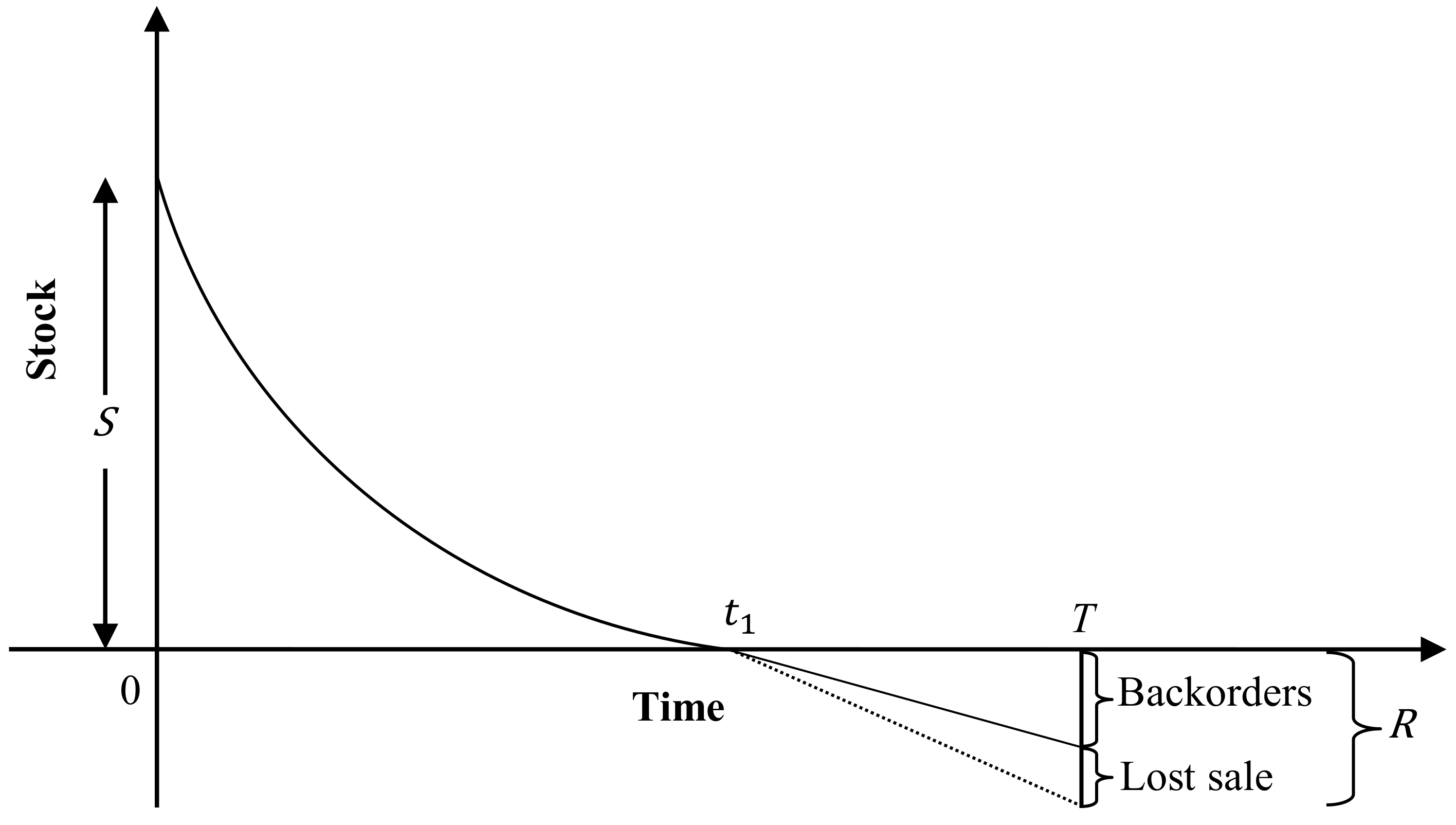
3.1. Problem Description

The goal of all entrepreneurs is to maximize profits in today’s competitive business world or to minimize the total cost of the chain. Retailing is a distribution system that structures a huge piece of the supply chain. Retailers purchasing products from suppliers and then selling them to customers is a natural process. Here is an explanation of how a retailer uses different customer management techniques and technologies to make a profit in business as well as retain the customer for a long time. After purchasing products from the supplier, the retailer stores them in his warehouse until they are sold. At this time, some products are perishable for a variety of reasons, so he uses preservation technologies for long-term preservation. The problem is to determine the costs for a whole cycle and the factors that influence whether costs go up or down.

3.2. Assumptions

The following assumptions are used in the development of the model:

• The demand for the product follows a constant pattern;
• Due to impatient customers, the demand during stockout is partially lost;
• The backlogged demand is satisfied with the arrival of the next lot;
• The products are deteriorating in nature;
• There is no replacement of deteriorated items;

Preservation technology is applied to reduce the existing rate of deterioration. The reduced deterioration rate is a function of the preservation technology cost $\xi$ such that:

$$m\left(\xi \right)=K\left(1-e^{-\xi x}\right),x\ge 0$$

where x is the coefficient which is representing the efficiency of preservation technology and $K$ is the highest reducible rate of deterioration.

4. Model Formulation

In this section, based on the advance payment strategy, there are two cases. Section 4.1 considers the case when advance payment is absent; Section 4.2 considers the case with advance payment.

4.1. Case I (Without Advance Payment)

In the beginning, the retailer orders the products from the supplier. The supplier then starts delivering the products during the lead time and the delivery of the total amount of ordered products is completed at $t=0$. In this case, the supplier does not offer any advance payment opportunity to the retailer, so the retailer has to pay the entire purchase price at once after the full delivery of the ordered products. Initially, with full stock in hand, the retailer starts to sell products to the customers. Due to customer demand and deterioration, the inventory starts to decline over time and the stock runs out at $t=t_1$ (See Figure 1). As a result, some customers switch to other shops to purchase products, and the retailer sees a loss in demand. Here, the retailer focuses on preservation technology to preserve products for a long time with optimum investment to secure a good profit margin.

The rate of change of inventory during the positive stock period $[0,t_1]$ and shortage period $[t_1,T]$ is governed by the differential equations:

$$\frac{d{I}_1}{dt}\left(t\right)+\left(\theta -m\right)I_1\left(t\right)=-D, 0\le t\le t_1$$

(1)

$$\frac{d{I}_2}{dt}\left(t\right)=-\delta D, t_1\le t\le T$$

(2)

With conditions:

$$I_1\left(0\right)=S, I_1\left(t_1\right)=0, I_2\left(t_1\right)=0, I_2\left(T\right)=-R$$

By solving Equations (1) and (2), and using the given conditions, we get:

$$I_1\left(t\right)=\frac{D}{\theta -m}\left(-1+e^{\left(\theta -m\right)\left(t_1-t\right)}\right)$$

(3)

$$I_2\left(t\right)=\delta D\left(t_1-t\right)$$

(4)

Using $I_1\left(0\right)=S$ Equation (3), the retailer’s initial stock is obtained.

$$S=\frac{D}{\theta -m}\left[e^{\left(\theta -m\right)t_1}-1\right]$$

(5)

Using $I_2\left(\mathrm{T}\right)=-R$ in Equation (4), the amount of shortage is obtained.

$$R=\delta D\left(T-t_1\right)$$

(6)

Thus, the total ordered amount per cycle is:

$$Q=S+R=\frac{D}{\theta -m}\left[e^{\left(\theta -m\right)t_1}-1\right]+\delta D\left(T-t_1\right)$$

(7)

Ordering cost: The retailer has to spend some money to process the order depending on the type of material, the quantity ordered, and the source of the supplier. Let $c_o$ be the order cost per cycle. Then:

$$OC=c_o$$

(8)

Purchase cost: If the purchase price per unit of product is $c_p$, then the retailer’s total purchase cost for $Q$ quantity of product will be:

$$PC=c_{p}Q=c_p\left[\frac{-D}{\theta -m}+\frac{D}{\theta -m}{e}^{\left(\theta -m\right)t_1}+\delta D\left(T-t_1\right)\right]$$

(9)

Holding Cost: Holding cost is the cost of keeping the goods in the warehouse from the time they are received until all the products are sold. If the holding cost per unit time is $c_h$, then the total holding cost for storing the products in the warehouse from time 0 to $t_1$ will be:

$$HC=c_h\underset{0}{\overset{t_1}{{\displaystyle \int }}}{I}_1\left(t\right)dt=c_h\frac{D}{{\left(\theta -m\right)}^2}\left[-1-t_1\left(\theta -m\right)+e^{\left(\theta -m\right)\left(t_1\right)}\right]$$

(10)

Shortage Cost: At the point when the interest for a product surpasses its provided amount, a shortage happens. We can see from this figure that the shortage starts at time $t_1$. If $c_{\mathrm{s}}$ be the shortage cost per unit, then the total shortage cost is:

$$SC=c_s\underset{t_1}{\overset{T}{{\displaystyle \int }}}-I_2\left(t\right)dt=c_s\delta D\left[\frac{t_1{}^2}{2}-t_{1}T+\frac{T^2}{2}\right]$$

(11)

Lost Sale Cost: This refers to the cost associated with a situation when retailers lose opportunities to sell because products are out of stock. If $c_l$ be the lost sale cost per unit, then the total lost sale cost is:

$$LSC=c_l{{\displaystyle \int }}_{t_1}^T\left(1-\delta \right)D dt=c_l\left(1-\delta \right)D\left[T-t_1\right]$$

(12)

Preservation Cost: This refers to the cost of investing in preservation technology to reduce product degradation. If $\xi$ be the preservation technology cost per unit time, then the total preservation cost can be written as:

$$PRC=\xi T$$

(13)

Finally, total cost is the summation of all costs, i.e.:

$$X=OC+PC+HC+SC+LSC+PRC.$$

(14)

Therefore, the total cost per cycle is:

$$TC\left(\xi ,T\right)=\frac{X}{T}=\frac{1}{T}\left[\begin{array}{c}{c}_0+c_p\left\{\begin{array}{c}\frac{-D}{\theta -m}+\frac{D}{\theta -m}{e}^{\left(\theta -m\right)t_1}\\ +\delta D\left(T-t_1\right)\end{array}\right\}\\ +c_h\frac{D}{{\left(\theta -m\right)}^2}\left[-1-t_1\left(\theta -m\right)+e^{\left(\theta -m\right)\left(t_1\right)}\right]\\ +c_s\delta D\left[\frac{t_1{}^2}{2}-t_{1}T+\frac{T^2}{2}\right]\\ +c_l\left(1-\delta \right)D\left[T-t_1\right]+\xi T\end{array}\right]$$

(15)

Proposition 1.

The cost function $TC\left(\xi T\right)$ in Equation (15) states the convexity in $T$ for any specific $\xi >0$ and entails a unique solution $T^{\ast }$.

Proof. 

Differentiating the cost function $TC\left(\xi T\right)$ in Equation (15) with respect to T, we get:

$$\frac{\partial TC}{\partial T}=\left[\begin{array}{c}\frac{1}{T^2}\left\{\begin{array}{c}{c}_h\frac{D}{{\left(\theta -m\right)}^2}-c_0-c_p\frac{D}{\theta -m}\left[e^{\left(\theta -m\right)t_1}-1\right]+c_h\frac{D{t}_1}{\left(\theta -m\right)}\\ +c_h\frac{D{e}^{\left(\theta -m\right)\left(t_1\right)}}{{\left(\theta -m\right)}^2}-c_{s}D\delta \frac{t_1{}^2}{2}-c_l\delta D{t}_1+c_p\delta D{t}_1\end{array}\right\}\\ +\frac{c_{s}D\delta }{2}+\frac{1}{T}{c}_{l}D{t}_1\end{array}\right]$$

(16)

To evaluate the value of $T$,$\frac{\partial TC}{\partial T}=0$. Then we get:

$$T=\frac{-{\lambda }_2\pm \sqrt{\left({\lambda }_2{}^2-2C_s\delta D{\lambda }_1\right)}}{C_s\delta D}$$

where

$${\lambda }_1=\left\{\begin{array}{c}{c}_h\frac{D}{{\left(\theta -m\right)}^2}-c_0-c_p\frac{D}{\theta -m}\left[e^{\left(\theta -m\right)t_1}-1\right]+c_h\frac{D{t}_1}{\left(\theta -m\right)}\\ +c_h\frac{D{e}^{\left(\theta -m\right)\left(t_1\right)}}{{\left(\theta -m\right)}^2}-c_{s}D\delta \frac{t_1{}^2}{2}-c_l\delta D{t}_1+c_p\delta D{t}_1\end{array}\right\} \mathrm{and} {\lambda }_2=c_{l}D{t}_1.$$

Ignoring the negative value, the required value of $T$ is considered as follows:

$$T=\frac{-{\lambda }_2+\sqrt{{\lambda }_2{}^2-2C_s\delta D{\lambda }_1}}{C_s\delta D}=T^{\ast }$$

(17)

Now differentiating Equation (16) with respect to $T$ we get:

$$\frac{{\partial }^{2}TC}{\partial T^2}=\frac{2}{T^3}\left[\begin{array}{c}{c}_0+c_p\frac{D}{\theta -m}\left[e^{\left(\theta -m\right)t_1}-1\right]+c_h\frac{D}{{\left(\mathsf{\theta }-\mathrm{m}\right)}^2}{\mathrm{e}}^{\left(\mathsf{\theta }-\mathrm{m}\right)\left({\mathrm{t}}_1\right)}+c_s\mathsf{\delta }\mathrm{D}{\mathrm{t}}_1{}^2\\ +c_l\mathrm{D}{\mathrm{t}}_1\left(\mathsf{\delta }-1\right)-c_p\delta D{t}_1-c_h\frac{D}{{\left(\theta -m\right)}^2}\left[1+\left(\theta -m\right)t_1\right]\end{array}\right]$$

(18)

Expanding Equation (18) in Taylor’s series (similar to [36]) and then substituting the value of $T=T^{\ast }$, we get:

$${\left[\frac{{\partial }^{2}TC}{\partial T^2}\right]}_{T=T^{\ast }}=\frac{2}{T^{\ast }{}^3}\left[\begin{array}{c}{c}_0+\left(1-\mathsf{\delta }\right)\left(c_p-c_l\right)D{t}_1+c_s\mathsf{\delta }\mathrm{D}{\mathrm{t}}_1{}^2\end{array}\right].$$

(19)

□

Lemma  1.

The total cost function $TC\left(\xi T\right)$ in Equation (15) is strictly convex when $\left[\begin{array}{c}{c}_0+\left(1-\delta \right)\left(c_p-c_l\right)D{t}_1+c_s\delta D{t}_1{}^2\end{array}\right]>0.$

Proof. 

Since all the parameters are always assumed to be positive and the per unit purchase cost $C_p$ obviously greater than the per unit lost sale cost $C_l$, we consider that $\left[\begin{array}{c}{c}_0+\left(1-\delta \right)\left(c_p-c_l\right)D{t}_1+c_s\delta D{t}_1{}^2\end{array}\right]>0$.

If this condition is true, then the Equation (19) implies that ${\left[\frac{{\partial }^{2}TC}{\partial T^2}\right]}_{T=T^{\ast }}>0$ and hence satisfies the sufficient condition for the convexity of $TC\left(\xi T\right)$. □

Proposition 2.

The cost function $TC\left(\xi T\right)$ in Equation (15) states the convexity in $\xi$ for any specific $T>0$ and entails a unique solution ${\xi }^{\ast }$.

Proof. 

Similar to the proof of Proposition 1. □

Proposition 3.

The cost function $TC\left(\xi T\right)$ in Equation (15) indicates the convexity in $\left(\xi T\right)$ and entails a unique solution $\left({\xi }^{\ast }{T}^{\ast }\right)$.

Proof. 

Let us define the cost function Equation (15) as follows:

$$TC\left(T\right)=\frac{{\varphi }_1\left(\xi ,T\right)}{{\varphi }_2\left(T\right)}$$

(20)

where

$${\varphi }_1\left(\xi ,T\right)=\left[\begin{array}{c}{c}_0+c_p\left\{\begin{array}{c}\frac{-D}{\theta -m}+\frac{D}{\theta -m}{e}^{\left(\theta -m\right)t_1}\\ +\delta D\left(T-t_1\right)\end{array}\right\}\\ +c_h\frac{D}{{\left(\theta -m\right)}^2}\left[-1-t_1\left(\theta -m\right)+e^{\left(\theta -m\right)\left(t_1\right)}\right]\\ +c_s\delta D\left[\frac{t_1{}^2}{2}-t_{1}T+\frac{T^2}{2}\right]\\ +c_l\left(1-\delta \right)D\left[T-t_1\right]+\xi T\end{array}\right] \mathrm{and} {\varphi }_2\left(T\right)=T>0.$$

(21)

According to Theorems 3.2.9 and 3.2.10 in [14], the fractional cost function in Equation (20) is strictly pseudo-convex if ${\varphi }_1\left(T\right)$ is non-negative, differentiable, and strictly convex, and ${\varphi }_2\left(T\right)$ is positive, differentiable, and concave.

Now taking the first order derivative of ${\varphi }_1\left(T\right)$ with respect to T, we have:

$$\frac{\partial {\varphi }_1\left(T\right)}{\partial T}=c_p\delta D+c_s\delta D\left(T-t_1\right)+c_l\left(1-\delta \right)D+\xi$$

(22)

To find the value of T, place $\frac{\partial TC}{\partial T}=0$, which implies that:

$$T=\omega -\frac{\xi }{c_s\delta D}=T^{\ast }$$

(23)

where $\omega =\frac{\delta \left(c_s{t}_1+c_l-c_p\right)-c_l}{c_s\delta }$.

Now substituting the value of T in Equation (21), we get:

$${\varphi }_1\left(\xi \right)=\left[\begin{array}{c}{c}_0+c_p\left\{\begin{array}{c}\frac{-D}{\theta -m}+\frac{D}{\theta -m}{e}^{\left(\theta -m\right)t_1}\\ +\delta D\left(\omega -\frac{\xi }{c_s\delta D}-t_1\right)\end{array}\right\}\\ +c_h\frac{D}{{\left(\theta -m\right)}^2}\left[-1-t_1\left(\theta -m\right)+e^{\left(\theta -m\right)\left(t_1\right)}\right]\\ +c_s\delta D\left[\frac{t_1{}^2}{2}-t_1\left(\omega -\frac{\xi }{c_s\delta D}\right)+\frac{{\left(\omega -\frac{\xi }{c_s\delta D}\right)}^2}{2}\right]\\ +c_l\left(1-\delta \right)D\left[\omega -\frac{\xi }{c_s\delta D}-t_1\right]+\left(\xi \ast \left(\omega -\frac{\xi }{c_s\delta D}\right)\right)\end{array}\right]$$

(24)

which becomes the function of $\xi$.

Let us take the first derivative of Equation (24) with respect to $\xi$, we get:

$$\frac{\partial {\varphi }_1\left(\xi \right)}{\partial \xi }=\left[\begin{array}{c}-\frac{1}{c_s\delta }\left[c_p\delta +c_l\left(1-\delta \right)+\frac{\xi }{D}\right]+\frac{t_1}{2}\\ -kxD\frac{e^{-\xi x}}{{\left(\theta -m\right)}^2}\left[c_p-c_h{t}_1+\frac{2c_h}{\left(\theta -m\right)}\right]\\ -\frac{kxD}{\left(\theta -m\right)}{e}^{-\xi x+\left(\theta -m\right)t_1}\left[c_p{t}_1-\frac{\left(c_p-c_h\right)t_1}{\left(\theta -m\right)}-\frac{2c_h}{{\left(\theta -m\right)}^2}\right]\end{array}\right]$$

(25)

Equate this to zero for finding the value of $\xi ={\xi }^{\ast }$.

Now differentiating Equation (25) with respect to $\xi$, we get:

$$\frac{{\partial }^2{\varphi }_1\left(\xi \right)}{\partial {\xi }^2}=\left[\begin{array}{c}k{x}^{2}D\frac{e^{-\xi x}}{{\left(\theta -m\right)}^3}\left[\left(c_p-c_h{t}_1\right)\left(\theta -m\right)+2c_h\right]\\ +2k{x}^{2}D{t}_1\left(k{t}_1{e}^{-\xi x}-1\right)\frac{e^{-\xi x+\left(\theta -m\right)t_1}}{{\left(\theta -m\right)}^3}\left[\begin{array}{c}\left(c_p-c_h\right)\left(\theta -m\right)\\ +2c_h-c_p{\left(\theta -m\right)}^2\end{array}\right]\\ +2k^2{x}^{2}D{t}_1\frac{e^{-2\xi x+\left(\theta -m\right)t_1}}{{\left(\theta -m\right)}^4}\left[\left(c_p-c_h\right)\left(\theta -m\right)+3c_h-c_p{\left(\theta -m\right)}^2\right]\\ -\left\{\frac{1}{c_s\delta D}+2k^2{x}^{2}D\frac{e^{-2\xi x}}{{\left(\theta -m\right)}^4}\left[\left(c_p-c_h{t}_1\right)\left(\theta -m\right)+3c_h\right]\right\}\end{array}\right]$$

(26)

Then, after the submission of the value of $\xi ={\xi }^{\ast }$ in Equation (26), we simply write this as follows:

$${\left[\frac{{\partial }^2{\varphi }_1\left(\xi \right)}{\partial {\xi }^2}\right]}_{\xi ={\xi }^{\ast }}=F_1\left({\xi }^{\ast }\right)-F_2\left({\xi }^{\ast }\right)$$

(27)

where

$$F_1\left({\xi }^{\ast }\right)=\left[\begin{array}{c}k{x}^{2}D\frac{e^{-{\xi }^{\ast }x}}{{\left(\theta -m\right)}^3}\left[\left(c_p-c_h{t}_1\right)\left(\theta -m\right)+2c_h\right]\\ +2k{x}^{2}D{t}_1\left(k{t}_1{e}^{-{\xi }^{\ast }x}-1\right)\frac{e^{-{\xi }^{\ast }x+\left(\theta -m\right)t_1}}{{\left(\theta -m\right)}^3}\left[\begin{array}{c}\left(c_p-c_h\right)\left(\theta -m\right)\\ +2c_h-c_p{\left(\theta -m\right)}^2\end{array}\right]\\ +2k^2{x}^{2}D{t}_1\frac{e^{-2{\xi }^{\ast }x+\left(\theta -m\right)t_1}}{{\left(\theta -m\right)}^4}\left[\left(c_p-c_h\right)\left(\theta -m\right)+3c_h-c_p{\left(\theta -m\right)}^2\right]\end{array}\right]$$

and

$$F_2\left({\xi }^{\ast }\right)=\frac{1}{c_s\delta D}+2k^2{x}^{2}D\frac{e^{-2{\xi }^{\ast }x}}{{\left(\theta -m\right)}^4}\left[\left(c_p-c_h{t}_1\right)\left(\theta -m\right)+3c_h\right].$$

□

Lemma 2.

The total cost function $TC\left(\xi ,T\right)$ in Equation (15) is strictly convex if $F_1\left({\xi }^{\ast }\right)>F_2\left({\xi }^{\ast }\right)$ is satisfied.

Proof. 

If we notice both the functions $F_1\left({\xi }^{\ast }\right)$ and $F_2\left({\xi }^{\ast }\right)$, it is clearly observed that $F_1\left({\xi }^{\ast }\right)$ is the summation of some larger positive terms in comparison to $F_2\left({\xi }^{\ast }\right).$ Therefore, we can say that $F_1\left({\xi }^{\ast }\right)>F_2\left({\xi }^{\ast }\right)$. This condition implies that ${\left[\frac{{\partial }^2{\varphi }_1\left(\xi \right)}{\partial {\xi }^2}\right]}_{\xi ={\xi }^{\ast }}>0$ and declares the convexity of $TC\left(\xi ,T\right)$ for optimum ${\xi }^{\ast }$ and $T^{\ast }$. □

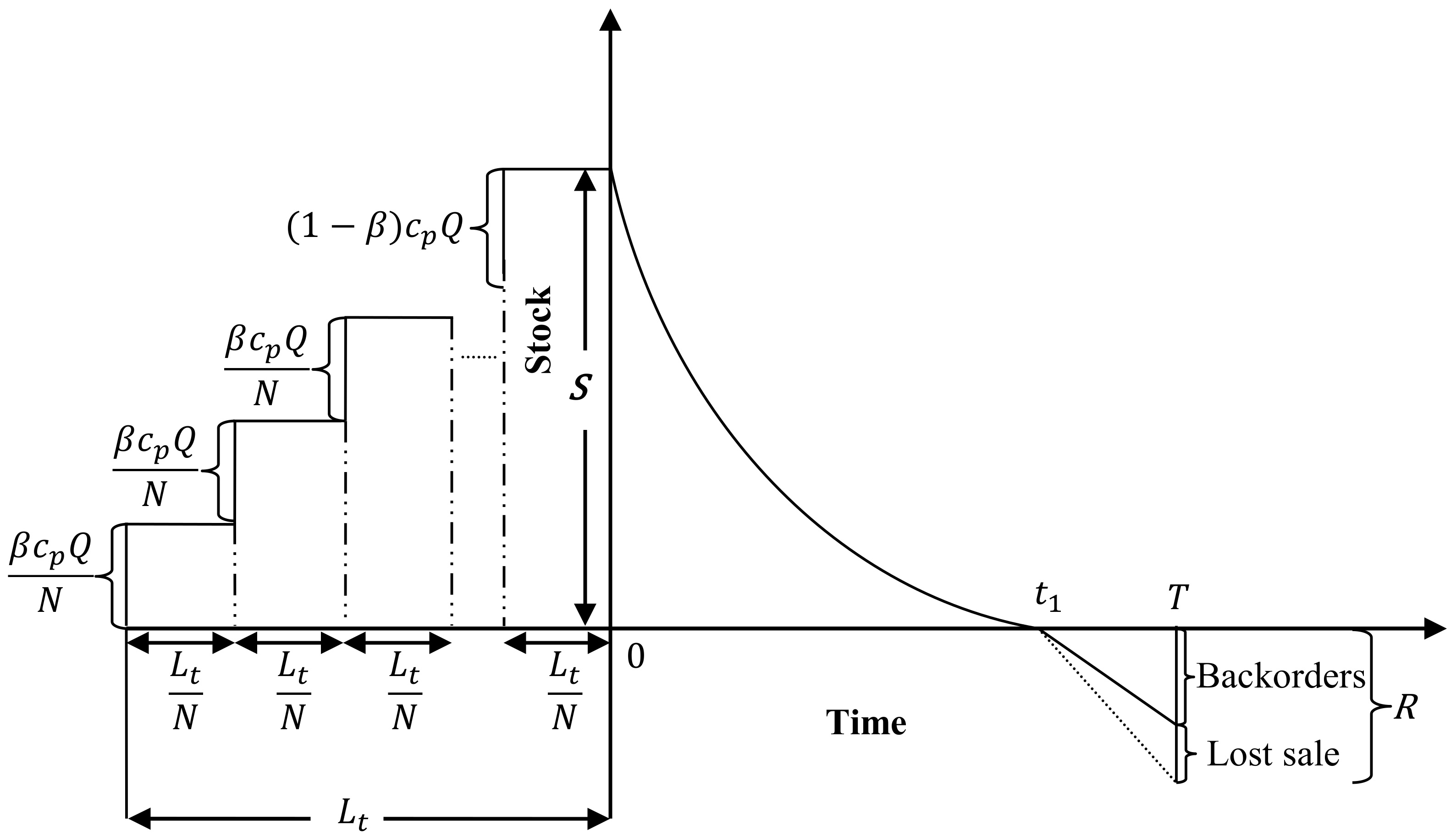
4.2. Case II (With Advance Payment)

In this case, there is an option for the retailer to accept the offer of an advance payment scheme proposed by the supplier, so the retailer does not need to pay the entire purchase price at once during the full delivery of the ordered product. He pays $\beta$ part of the total purchased price in $N$ number of installments within the lead time $L_t$, which is presented in Figure 2, and the remaining $\left(1-\beta \right)$ portion is to be paid at the time of receipt of the ordered products. The interest rate imposed on this pre-payment is $\tau$. At $t=0,$ the retailer’s warehouse becomes full of stock. After that, the inventory gradually starts to decline because of deterioration and customer demand and then finally becomes a vacuum at $t=t_1$. Therefore, shortage of products is seen during $[t_1,T]$.

Capital cost:

$$CC=\tau \left[\frac{\beta c_{p}Q}{N}\left(\frac{L_t}{N}\right)\left(1+2+\dots \dots +N\right)\right]=\left(\frac{N+1}{2N}\right)\beta L_t\tau c_{p}Q$$

$$=\left(\frac{N+1}{2N}\right)\beta L_t\tau c_p\left\{\begin{array}{c}\frac{-D}{\theta -m}+\frac{D}{\theta -m}{e}^{\left(\theta -m\right)t_1}+\delta D\left(T-t_1\right)\end{array}\right\}$$

(28)

Then the total cost per cycle becomes as follows:

$$TC=\frac{X}{T},\mathrm{where} X=OC+PC+HC+SC+LSC+PRC+CC$$

$$TC=\frac{1}{T}\left[\begin{array}{c}{c}_0+c_p\left\{\begin{array}{c}\frac{-D}{\theta -m}+\frac{D}{\theta -m}{e}^{\left(\theta -m\right)t_1}\\ +\delta D\left(T-t_1\right)\end{array}\right\}\\ +c_h\frac{D}{{\left(\theta -m\right)}^2}\left[-1-t_1\left(\theta -m\right)+e^{\left(\theta -m\right)\left(t_1\right)}\right]\\ +c_s\delta D\left[\frac{t_1{}^2}{2}-t_{1}T+\frac{T^2}{2}\right]+c_l\left(1-\delta \right)D\left[T-t_1\right]+\xi T\\ +\left(\frac{N+1}{2N}\right)\beta L_t\tau c_p\left\{\begin{array}{c}\frac{-D}{\theta -m}+\frac{D}{\theta -m}{e}^{\left(\theta -m\right)t_1}\\ +\delta D\left(T-t_1\right)\end{array}\right\}\end{array}\right]$$

(29)

Proposition 4.

The cost function $TC\left(\xi ,T\right)$ in Equation (29) states the convexity in $T$ for any specific $\xi >0$ and entails a unique solution $T^{\ast }$.

Proof. 

The proof of this proposition is similar to that of Proposition 1. □

Proposition 5.

The cost function $TC\left(\xi ,T\right)$ in Equation (29) states the convexity in $\xi$ for any specific $T>0$ and entails a unique solution ${\xi }^{\ast }$.

Proof. 

Same as Proposition 4. □

Proposition 6. 

The cost function $TC\left(\xi ,T\right)$ in Equation (29) states the convexity in $\left(\xi ,T\right)$ and entails a unique solution $({\xi }^{\ast },T^{\ast })$.

Proof. 

Similar to that of Proposition 3. □

5. Numerical Illustrations

Some necessary data related to this model have been collected to validate the proposed model in real life. Profits are then numerically evaluated using those data which we have described in this section as examples. However, the total solution procedure is being visualized with the help of an algorithm.

5.1. Algorithm (For Case I)

Due to the high non-linearity in the cost function, a heuristic approach is presented in this section for Case I when taking single decision variables and another is taken as fixed.

Step 1:

Plug in all the associated values of the parameters.

Step 2:

When the situation

$\left[\begin{array}{c}{c}_0+c_s\mathsf{\delta }\mathrm{D}{\mathrm{t}}_1{}^2+\left(1-\mathsf{\delta }\right)\left(c_p-c_l\right)D{t}_1\end{array}\right]>0$ holds, there exists

$T^{\ast }$ for each cycle; if this form satisfies, proceed to Step 3; otherwise, proceed to Step 7.

Step 3:

Check $T=\frac{-{\lambda }_2+\surd \left({\lambda }_2{}^2-2C_s\delta D{\lambda }_1\right)}{C_s\delta D}=T^{\ast }$ with the help of Equation (17).

Step 4:

When $T^{\ast }$ accomplishes the sufficient condition for the optimum result indicated in Equation (19), then $T=T^{\ast }$ is the optimal outcome which minimizes Equation (15); if not, proceed to Step 7.

Step 5:

The order quantity can be determined from $Q^{\ast }=\frac{D}{\theta -m}\left[e^{\left(\theta -m\right)t_1}-1\right]+\delta D\left(T-t_1\right)$.

Step 6:

The total cost is calculated from Equation (15), and $T^{\ast }$ is premeditated from Equation (17).

Step 7:

End.

5.2. Case I (Without Advance Payment)

Example 1.

The following input parameters are considered for the model when an advance payment scheme is absent. Let $c_o=300, D=79.500,$ $\delta =0.6,$$\theta =0.4,$$t_1=0.8,$$c_h=3,$$c_p=15,$ $c_s=2,$$c_l=1.5,$$k=0.1,$$x=0.5$.

Then, by solving Equation (15) with the assistance of Lingo 17 software, the optimum values are $Q^{\ast }=240.260$, $T^{\ast }$ = 4.319, ${\xi }^{\ast }$ = 3.414, and $T{C}^{\ast }$ = 1102.281.

Figure 3 and Figure 4a,b show the concavity of the total cost function graphically.

Example 2.

When no steps have been taken to reduce the deterioration, i.e., when preservation technology is not applied:

By substituting $\xi =0$ in Equation (15), the optimum values are:

$$Q^{\ast }=247.351, T^{\ast }=4.414 \mathrm{and} T{C}^{\ast }=1107.993.$$

5.3. Case II (With Advance Payment)

Example 3.

Considering the same input parameters for Example 1 and some following additional parameters for the model when an advance payment scheme is present. Let $\beta =0.4,$$L_t=0.6,$ $\tau =0.1,$$N=4$.

By solving Equation (29) with the assistance of Lingo 17 software, the optimum values are:

$$Q^{\ast }=72.081, T^{\ast }=0.802, {\xi }^{\ast }=6.793, \mathrm{and} T{C}^{\ast }=1852.487.$$

Figure 5 shows the concavity of the total cost function graphically.

Example 4.

When no steps have been taken to reduce the deterioration, i.e., when preservation technology is not applied:

By substituting $\xi$ = 0 in Equation (29), the optimum values are:

$$Q^{\ast }=75.054, T^{\ast }=0.802 \mathrm{and} T{C}^{\ast }=1904.953.$$

5.4. Comparative Study

Figure 6 represents a comparison between the results of the model with advance payment and without advance payment. It can be seen that the costs incurred in each situation of case II are higher than in case I. This is because the retailer gets the benefit of paying in advance in a few installments, meaning that he does not have to pay the entire amount at once. In return, however, he will have to pay a certain amount as interest, based on the number of installments, which reduces the total cost of the business. From Figure 6, we can see that the result of case II is 68.06% higher than case I when preservation technology is present. Next, the situation with no investment in preservation technology displays a 71.93% increase in case II from case I. Overall, the highest cost is seen in both cases when preservation technology is not used, this being 2.83% higher in case II and 0.52% higher in case I.

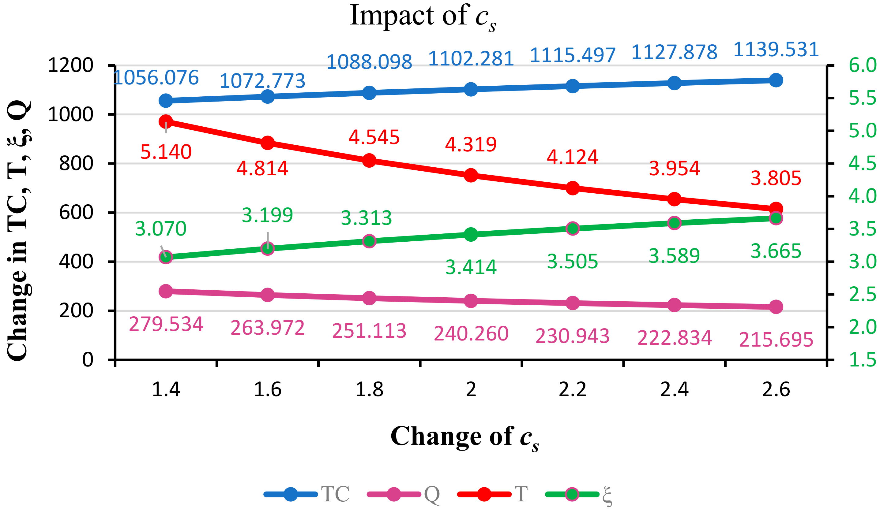
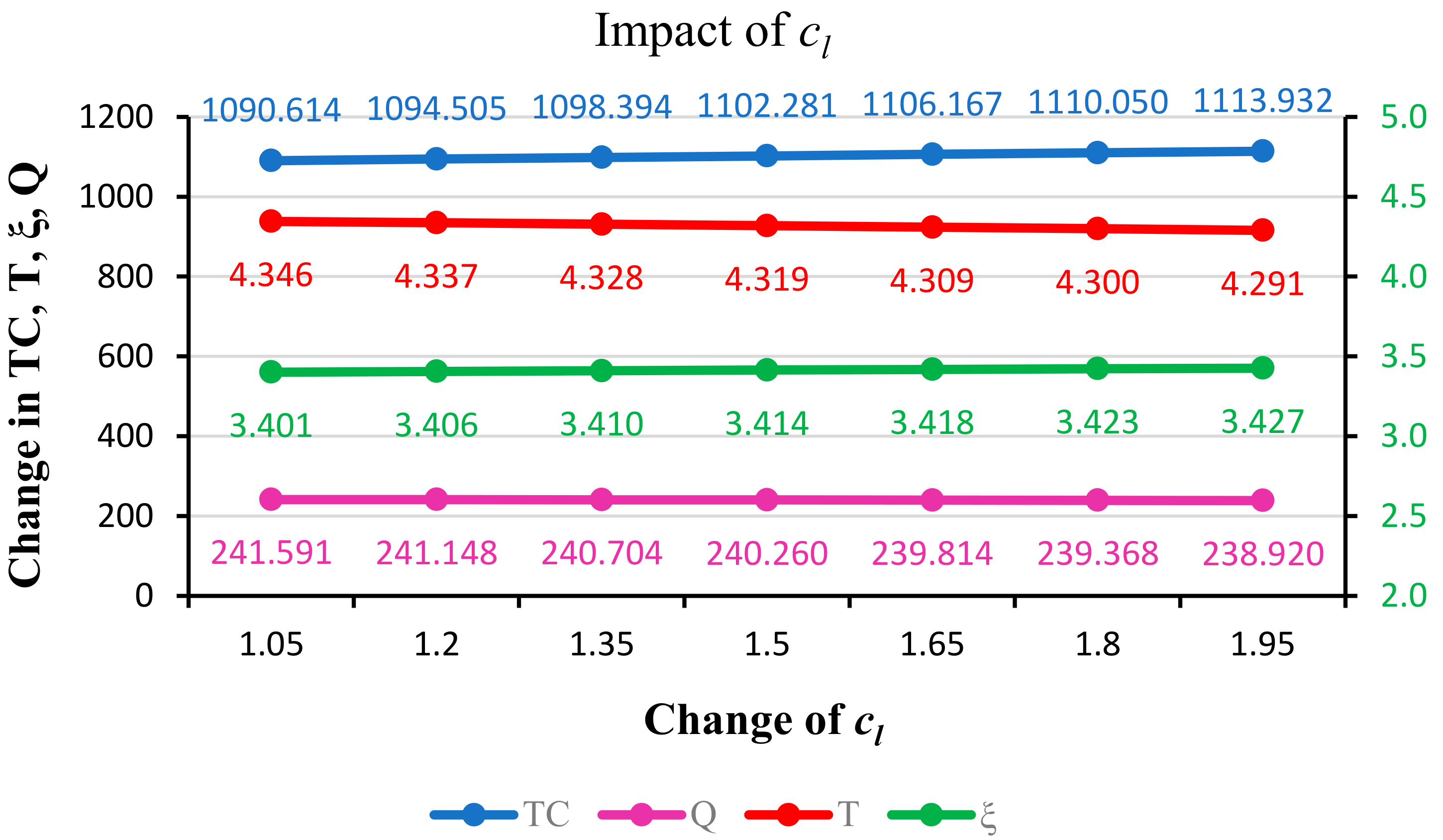
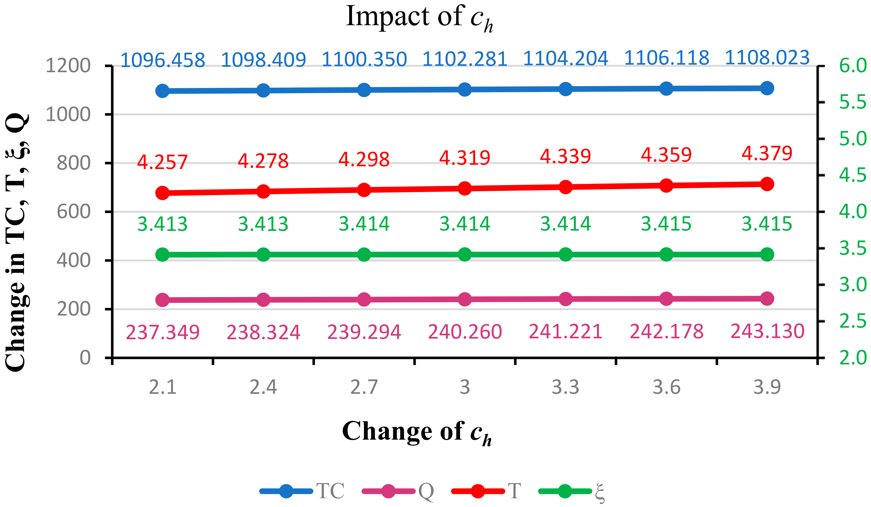
6. Sensitivity Analysis

The sensitivity analysis is performed in this section (Figure 7, Figure 8, Figure 9, Figure 10, Figure 11, Figure 12 and Figure 13). The total costs, replenishment cycles, preservation technology costs, and lot sizes are derived when different related parameters vary from −30% to 30%.

From Figure 7, the total cost, preservation technology cost and lot size are swelling steadily, owing to the augmentation of $\delta$. On the other hand, the replenishment cycle is declining slowly, owing to the growth of $\delta$. So, $\delta$ has both positive and negative impacts on the determined values. In reality, when a shortage is increased, the retailer does not need to hold the products. As a result, he can save some expenses which later decrease the cost to the retailer.

From Figure 8, we see that total cost, preservation technology cost, replenishment cycle and lot size are increasing gradually due to the rise of $\theta$. As the deterioration of products always decreases the amount of stock which has some value, it increases total costs; it is also observed that when the rate of deterioration increases, the preservation technology cost correspondingly increases.

Figure 9 shows that total cost, preservation technology cost, replenishment cycle, and lot size increase gradually due to the increment of $t_1$. With the increase of initial time, the deterioration period increases, and consequently the cost of preservation technology rises. As the non-shortage time or initial time augmented the order quantity, this also amplified because the chance to obtain the products at the right time upsurged.

Figure 10 shows that total cost, preservation technology cost, replenishment cycle, and lot size increase gradually due to the increment of $c_h$. From Figure 10, it is clear that when per unit holding cost increases, the total cost for the retailer also increases. As holding cost increases, it also means that the retailer holds the products for more time than is usual and consequently increases the preservation technology cost.

Figure 11 shows that total cost, preservation technology cost, replenishment cycle, and lot size increase gradually due to the increment of $c_p$. From Figure 11, it can be noticed that any increase in purchase cost will increase the total cost, and as the purchase cost increases, the retailer sets the selling price high. As a result, the length of total cycle length also increases. However, the preservation technology investment also needs to be implemented for a longer time.

Figure 12 shows that total cost and preservation technology cost are increasing gradually due to the increment of $c_s$. However, the opposite can be noticed for the total order quantity. On the other hand, the replenishment cycle and lot size are shrinking due to the growth of $c_s$. A significant impact is noticed for preservation technology investment, while a stable intensification is noticed for the replenishment cycle.

Figure 13 shows that total cost and preservation technology cost are increasing gradually due to the increment of $c_l$. Since the retailer is unable to satisfy some demand, as a result, the customers move to other sources, so some additional amounts are added to the total cost. On the other hand, replenishment cycle and lot size are decreasing due to the increment of $c_l$.

7. Managerial Insights

Deterioration of products is always an essential issue in proper inventory management. An advance payment scheme and preservation technology provide some flexibility to the retailer in order to deal with customers to secure a good profit margin. This study provides some managerial insights for the practitioners as follows:

(i)

One can quickly know how much and for how long one will have to invest in preservation technology to reduce product deterioration.

(ii)

An advance payment system creates flexibility for the retailer to deal with customers efficiently, although the capital is slightly lower compared to the general case. Moreover, advance payment always requires the retailer to complete the purchase in time, as some parts of the purchase cost have already been deposited in the supplier’s account. Thus, it sometimes helps to make a rigid decision in purchasing items from suppliers.

In addition, the simultaneous integration of preservation technology and an advance payment scheme will provide unique outputs in ordering decisions and logistics management.

8. Conclusions and Future Prospects

An inventory model for a retailer with constant demand under an advance payment policy has been proposed in this paper. To manage deterioration, a preservation technology has been successfully implemented which provides some managerial insights for the retailer. Preservation technology allows a lengthened product life and works successfully to curb deterioration. This model reveals some pricing strategies and gives a clear idea about how advertisement frequency can affect a retailer’s profits. Under the intensification of retailer profit, advance payment has been successfully implemented, and showed a significant result that helps to reduce the default risk and cancellation of orders. Some significant results have been developed considering a simultaneous investment in preservation and an advance payment scheme with the effect of advertisement. Prior studies also provide some theoretical analysis to validate the model with a numerical sensitivity analysis of key parameters.

This model can be extended in numerous ways; for instance, one can develop this model by implementing a trade credit policy (single- [40] or two-level [3]). It will be an exciting extension if environmental [7] factors can be added to the proposed model. One might also include stochastic deterioration [41] and a multi-item deteriorating inventory in the model [42].

References

1. Harris, F.W. How many parts to make at once. Fact. Mag. Manag. 1913, 10, 135–136. [Google Scholar] [CrossRef]
2. Mishra, U.; Tijerina-Aguilera, J.; Tiwari, S.; Cárdenas-Barrón, L.E. Retailer’s Joint Ordering, Pricing, and Preservation Technology Investment Policies for a Deteriorating Item under Permissible Delay in Payments. Math. Probl. Eng. 2018, 2018, 1–14. [Google Scholar] [CrossRef]
3. Lashgari, M.; Taleizadeh, A.A.; Sana, S.S. An inventory control problem for deteriorating items with back-ordering and financial considerations under two levels of trade credit linked to order quantity. J. Ind. Manag. Optim. 2015, 12, 1091–1119. [Google Scholar] [CrossRef] [Green Version]
4. Sethi, V.; Sethi, S. Processing of Fruits and Vegetables for Value Addition; Indus Publishing: New Delhi, India, 2006; ISBN 8173871809. [Google Scholar]
5. Dye, C.-Y. The effect of preservation technology investment on a non-instantaneous deteriorating inventory model. Omega 2013, 41, 872–880. [Google Scholar] [CrossRef]
6. Soni, H.N. Optimal replenishment policies for non-instantaneous deteriorating items with price and stock sensitive demand under permissible delay in payment. Int. J. Prod. Econ. 2013, 146, 259–268. [Google Scholar] [CrossRef]
7. Mashud, A.H.M.; Roy, D.; Daryanto, Y.; Ali, M.H. A Sustainable Inventory Model with Imperfect Products, Deterioration, and Controllable Emissions. Mathematics 2020, 8, 2049. [Google Scholar] [CrossRef]
8. Li, G.; He, X.; Zhou, J.; Wu, H. Pricing, replenishment and preservation technology investment decisions for non-instantaneous deteriorating items. Omega 2019, 84, 114–126. [Google Scholar] [CrossRef]
9. Dye, C.-Y.; Hsieh, T.-P. An optimal replenishment policy for deteriorating items with effective investment in preservation technology. Eur. J. Oper. Res. 2012, 218, 106–112. [Google Scholar] [CrossRef]
10. Taleizadeh, A.A.; Pourmohammad-Zia, N.; Konstantaras, I. Partial linked-to-order delayed payment and life time effects on decaying items ordering. Oper. Res. 2021, 21, 2077–2099. [Google Scholar] [CrossRef]
11. Taleizadeh, A.A.; Tavakoli, S.; San-José, L.A. A lot sizing model with advance payment and planned backordering. Ann. Oper. Res. 2018, 271, 1001–1022. [Google Scholar] [CrossRef]
12. Shi, Y.; Zhang, Z.; Chen, S.-C.; Cárdenas-Barrón, L.E.; Skouri, K. Optimal replenishment decisions for perishable products under cash, advance, and credit payments considering carbon tax regulations. Int. J. Prod. Econ. 2020, 223, 107514. [Google Scholar] [CrossRef]
13. Mashud, A.H.M.; Wee, H.-M.; Sarkar, B.; Chiang Li, Y.-H. A sustainable inventory system with the advanced payment policy and trade-credit strategy for a two-warehouse inventory system. Kybernetes 2021, 50, 1321–1348. [Google Scholar] [CrossRef]
14. Cambini, A.; Martein, L. Generalized Convexity and Optimization; Lecture Notes in Economics and Mathematical Systems; Springer: Berlin/Heidelberg, Germany, 2009; Volume 616, ISBN 978-3-540-70875-9. [Google Scholar]
15. Harris, F.W. What Quantity to Make at Once. Libr. Fact. Manag. Oper. Costs 1915, 5, 47–52. [Google Scholar]
16. Ghare, P.M.; Schrader, G.F. A model for an exponentially decaying inventory. J. Ind. Eng. 1963, 14, 238–243. [Google Scholar]
17. Skouri, K.; Papachristos, S. A continuous review inventory model, with deteriorating items, time-varying demand, linear replenishment cost, partially time-varying backlogging. Appl. Math. Model. 2002, 26, 603–617. [Google Scholar] [CrossRef]
18. Li, R.; Teng, J.-T.; Zheng, Y. Optimal credit term, order quantity and selling price for perishable products when demand depends on selling price, expiration date, and credit period. Ann. Oper. Res. 2019, 280, 377–405. [Google Scholar] [CrossRef]
19. Tiwari, S.; Cárdenas-Barrón, L.E.; Goh, M.; Shaikh, A.A. Joint pricing and inventory model for deteriorating items with expiration dates and partial backlogging under two-level partial trade credits in supply chain. Int. J. Prod. Econ. 2018, 200, 16–36. [Google Scholar] [CrossRef]
20. Mashud, A.H.M. An EOQ deteriorating inventory model with different types of demand and fully backlogged shortages. Int. J. Logist. Syst. Manag. 2020, 36, 16. [Google Scholar] [CrossRef]
21. Udayakumar, R.; Geetha, K.V.; Sana, S.S. Economic ordering policy for non-instantaneous deteriorating items with price and advertisement dependent demand and permissible delay in payment under inflation. Math. Methods Appl. Sci. 2021, 44, 7697–7721. [Google Scholar] [CrossRef]
22. Mashud, A.H.M.; Wee, H.-M.; Huang, C.-V.; Wu, J.-Z. Optimal Replenishment Policy for Deteriorating Products in a Newsboy Problem with Multiple Just-in-Time Deliveries. Mathematics 2020, 8, 1981. [Google Scholar] [CrossRef]
23. Mashud, A.M.; Hasan, R. An Economic Order Quantity model for Decaying Products with the Frequency of Advertisement, Selling Price and Continuous Time Dependent Demand under Partially Backlogged Shortage. Int. J. Supply Oper. Manag. 2019, 6, 296–314. [Google Scholar] [CrossRef]
24. Das, S.C.; Zidan, A.; Manna, A.K.; Shaikh, A.A.; Bhunia, A.K. An application of preservation technology in inventory control system with price dependent demand and partial backlogging. Alexandria Eng. J. 2020, 59, 1359–1369. [Google Scholar] [CrossRef]
25. Teng, J.-T.; Cárdenas-Barrón, L.E.; Chang, H.-J.; Wu, J.; Hu, Y. Inventory lot-size policies for deteriorating items with expiration dates and advance payments. Appl. Math. Model. 2016, 40, 8605–8616. [Google Scholar] [CrossRef]
26. Lashgari, M.; Taleizadeh, A.A.; Sadjadi, S.J. Ordering policies for non-instantaneous deteriorating items under hybrid partial prepayment, partial trade credit and partial backordering. J. Oper. Res. Soc. 2018, 69, 1167–1196. [Google Scholar] [CrossRef]
27. Taleizadeh, A.A. Lot-sizing model with advance payment pricing and disruption in supply under planned partial backordering. Int. Trans. Oper. Res. 2017, 24, 783–800. [Google Scholar] [CrossRef]
28. Lashgari, M.; Taleizadeh, A.A.; Ahmadi, A. Partial up-stream advanced payment and partial down-stream delayed payment in a three-level supply chain. Ann. Oper. Res. 2016, 238, 329–354. [Google Scholar] [CrossRef]
29. Maiti, A.K.; Maiti, M.K.; Maiti, M. Inventory model with stochastic lead-time and price dependent demand incorporating advance payment. Appl. Math. Model. 2009, 33, 2433–2443. [Google Scholar] [CrossRef]
30. Chen, S.-C.; Teng, J.-T. Retailer’s optimal ordering policy for deteriorating items with maximum lifetime under supplier’s trade credit financing. Appl. Math. Model. 2014, 38, 4049–4061. [Google Scholar] [CrossRef]
31. Taleizadeh, A.A. An economic order quantity model for deteriorating item in a purchasing system with multiple prepayments. Appl. Math. Model. 2014, 38, 5357–5366. [Google Scholar] [CrossRef]
32. Khedlekar, U.K.; Shukla, D.; Namdeo, A. Pricing policy for declining demand using item preservation technology. Springerplus 2016, 5, 1957. [Google Scholar] [CrossRef] [Green Version]
33. Shah, N.H.; Vaghela, C.R. Economic order quantity for deteriorating items under inflation with time and advertisement dependent demand. Opsearch 2017, 54, 168–180. [Google Scholar] [CrossRef]
34. Tavakoli, S.; Taleizadeh, A.A. An EOQ model for decaying item with full advanced payment and conditional discount. Ann. Oper. Res. 2017, 259, 415–436. [Google Scholar] [CrossRef]
35. Mashud, A.; Khan, M.; Uddin, M.; Islam, M. A non-instantaneous inventory model having different deterioration rates with stock and price dependent demand under partially backlogged shortages. Uncertain Supply Chain Manag. 2018, 6, 49–64. [Google Scholar] [CrossRef]
36. Noori-daryan, M.; Taleizadeh, A.A.; Govindan, K. Joint replenishment and pricing decisions with different freight modes considerations for a supply chain under a composite incentive contract. J. Oper. Res. Soc. 2018, 69, 876–894. [Google Scholar] [CrossRef]
37. Soni, H.N.; Suthar, D.N. Pricing and inventory decisions for non-instantaneous deteriorating items with price and promotional effort stochastic demand. J. Control Decis. 2019, 6, 191–215. [Google Scholar] [CrossRef]
38. Li, R.; Liu, Y.; Teng, J.-T.; Tsao, Y.-C. Optimal pricing, lot-sizing and backordering decisions when a seller demands an advance-cash-credit payment scheme. Eur. J. Oper. Res. 2019, 278, 283–295. [Google Scholar] [CrossRef]
39. Das, S.; Khan, M.A.A.; Mahmoud, E.E.; Abdel-Aty, A.H.; Abualnaja, K.M.; Shaikh, A.A. A production inventory model with partial trade credit policy and reliability. Alexandria Eng. J. 2021, 60, 1325–1338. [Google Scholar] [CrossRef]
40. Taleizadeh, A.A.; Lashgari, M.; Akram, R.; Heydari, J. Imperfect economic production quantity model with upstream trade credit periods linked to raw material order quantity and downstream trade credit periods. Appl. Math. Model. 2016, 40, 8777–8793. [Google Scholar] [CrossRef]
41. Pervin, M.; Roy, S.K.; Weber, G.-W. Analysis of inventory control model with shortage under time-dependent demand and time-varying holding cost including stochastic deterioration. Ann. Oper. Res. 2018, 260, 437–460. [Google Scholar] [CrossRef]
42. Pervin, M.; Kumar Roy, S.; Wilhelm Weber, G. Multi-item deteriorating two-echelon inventory model with price- and stock-dependent demand: A trade-credit policy. J. Ind. Manag. Optim. 2017, 13, 1–29. [Google Scholar] [CrossRef]
Figure 1. Graphical representation of the proposed inventory model for Case I.
Processes 10 00546 g001
Figure 2. Graphical representation of the proposed inventory model for Case II.
Processes 10 00546 g002
Figure 3. The relationship between T, ξ, and TC.
Processes 10 00546 g003
Figure 4. Total cost function (TC) regarding: (a) replenishment cycle (T); (b) preservation technology cost per unit time (ξ).
Processes 10 00546 g004
Figure 5. The relationship among T ,   ξ ,   and   T C .
Processes 10 00546 g005
Figure 6. Comparison between the models with advance payment and without advance payment.
Processes 10 00546 g006
Figure 7. The relationship among δ and TC ,   T ,   ξ , Q .
Processes 10 00546 g007
Figure 8. The relationship among θ and TC ,   T ,   ξ , Q .
Processes 10 00546 g008
Figure 9. The relationship among t 1 and TC ,   T ,   ξ , Q .
Processes 10 00546 g009
Figure 10. The relationship among c h and TC ,   T ,   ξ , Q .
Processes 10 00546 g010
Figure 11. The relationship among c p and TC ,   T ,   ξ , Q .
Processes 10 00546 g011
Figure 12. The relationship among c s and TC ,   T ,   ξ , Q .
Processes 10 00546 g012
Figure 13. The relationship among c l and TC ,   T ,   ξ , Q .
Processes 10 00546 g013